MACS: AN AGENT-BASED MEMETIC MULTIOBJECTIVE
OPTIMIZATION ALGORITHM APPLIED TO SPACE TRAJECTORY
DESIGN
Massimiliano Vasile – Federico Zuiani
Space Advanced Research Team, University of Strathclyde
James Weir Building 75 Montrose Street G1 1XJ, Glasgow, United Kingdom
[email protected], [email protected]
ABSTRACT
This paper presents an algorithm for multiobjective optimization that blends together a
number of heuristics. A population of agents combines heuristics that aim at exploring
the search space both globally and in a neighborhood of each agent. These heuristics
are complemented with a combination of a local and global archive. The novel
agent-based algorithm is tested at first on a set of standard problems and then on three specific
problems in space trajectory design. Its performance is compared against a number of
state-of-the-art multiobjective optimisation algorithms that use the Pareto dominance
as selection criterion: NSGA-II, PAES, MOPSO, MTS. The results demonstrate that
the agent-based search can identify parts of the Pareto set that the other algorithms
were not able to capture. Furthermore, convergence is statistically better although the
KEYWORDS
Multiobjective optimisation; trajectory optimisation; memetic algorithms; multiagent
systems.
1. INTRODUCTION
The design of a space mission steps through different phases of increasing complexity.
In the first phase, a trade-off analysis of several options is required. The trade-off
analysis compares and contrasts design solutions according to different criteria and
aims at selecting one or two options that satisfy mission requirements. In mathematical
terms, the problem can be formulated as a multiobjective optimization problem.
As part of the trade-off analysis, multiple transfer trajectories to the destination need to
be designed. Each transfer should be optimal with respect to a number of criteria. The
solution of the associated multiobjective optimization problem, has been addressed, by
many authors, with evolutionary techniques. Coverstone et al. [1] proposed the use
of multiobjective genetic algorithms for the optimal design of low-thrust trajectories.
Dachwald et al. proposed the combination of a neurocontroller and of a multiobjective
evolutionary algorithm for the design of low-thrust trajectories [2]. In 2005 a study
by Lee et al. [3] proposed the use of a Lyapunov controller with a multiobjective
evo-lutionary algorithm for the design of low-thrust spirals. More recently, Sch¨utze et al.
proposed some innovative techniques to solve multiobjective optimization problems
for multi-gravity low-thrust trajectories. Two of the interesting aspects of the work
of Sch¨utze et al. are the archiving ofϵ- and∆-approximated solutions, to the known best Pareto front [4], and the deterministic pre-pruning of the search space [5]. In
2009, Delnitz et al. [6] proposed the use of multiobjective subdivision techniques for
the design of low-thrust transfers to the halo orbits around theL2libration point in the
Earth-Moon system. Minisci et al. presented an interesting comparison between an
EDA-based algorithm, called MOPED, and NSGA-II on some constrained and
uncon-strained multi-impulse orbital transfer problems [7].
proposed. In particular, the search for Pareto optimal solutions is carried out globally
by a population of agents implementing classical social heuristics and more locally by
a subpopulation implementing a number of individualistic actions. The reconstruction
of the set of Pareto optimal solutions is handled through two archives: a local and a
global one.
The individualistic actions presented in this paper are devised to allow each agent to
independently converge to the Pareto optimal set. Thus creating its own partial
repre-sentation of the Pareto front. Therefore, they can be regarded as memetic mechanisms
associated to a single individual. It will be shown that individualistic actions
signifi-cantly improve the performance of the algorithm.
The algorithm proposed in this paper is an extension of the Multi-Agent Collaborative
Search (MACS), initially proposed in [8, 9], to the solution of multiobjective
optimisa-tion problems. Such an extension required the modificaoptimisa-tion of the selecoptimisa-tion criterion,
for both global and local moves, to handle Pareto dominance and the inclusion of new
heuristics to allow the agents to move toward and along the Pareto front. As part of
these new heuristics, this papers introduces a dual archiving mechanism for the
man-agement of locally and globally Pareto optimal solutions and an attraction mechanisms
that improves the convergence of the population.
The new algorithm is here applied to a set of known standard test cases and to three
space mission design problems. The space mission design cases in this paper consider
spacecraft equipped with a chemical engine and performing a multi-impulse transfer.
Although these cases are different from some of the above-mentioned examples, that
consider a low-thrust propulsion system, nonetheless the size and complexity of the
search space is comparable. Furthermore, it provides a first test benchmark for
multi-impulsive problems that have been extensively studied in the single objective case but
for which only few comparative studies exist in the multiobjective case [7].
The paper is organised as follows: section two contains the general formulation of the
problem, the third section starts with a general introduction to the multi-agent
collab-orative search algorithm and heuristics before going into some of the implementation
effec-tiveness of the heuristics implemented in MACS. The section briefly introduces the
algorithms against which MACS is compared and the two test benchmarks that are
used in the numerical experiments. It then defines the performance metrics and ends
with the results of the comparison.
2. PROBLEM FORMULATION
A general problem in multiobjective optimization is to find the feasible set of solutions
that satisfies the following problem:
min
x∈Df(x) (1)
whereDis a hyperrectangle defined asD ={xj | xj ∈[blj buj]⊆R, j = 1, ..., n
}
andfis the vector function:
f :D→Rm, f(x) = [f1(x), f2(x), ..., fm(x)]T (2)
The optimality of a particular solution is defined through the concept of dominance:
with reference to problem (1), a vectory ∈ D is dominated by a vector x ∈ D if
fj(x)< fj(y)for allj= 1, ..., m. The relationx≺ystates thatxdominatesy. Starting from the concept of dominance, it is possible to associate, to each solution in
a set, the scalar dominance index:
Id(xj) =|{i|i∧j∈Np∧xi≺xj}| (3)
where the symbol|.|is used to denote the cardinality of a set andNpis the set of the indices of all the solutions. All non-dominated and feasible solutions form the set:
X ={x∈D|Id(x) = 0} (4)
Therefore, the solution of problem (1) translates into finding the elements ofX. IfX
ofXis identified it makes sense to explore its neighborhood to look for other elements ofX. On the other hand, the set of non dominated solutions can be disconnected and its elements can form islands inD. Hence, restarting the search process in unexplored regions ofDcan increase the collection of elements ofX.
The setX is the Pareto set and the corresponding image in criteria space is the Pareto front. It is clear that inDthere can be more than oneXlcontaining solutions that are locally non-dominated, or locally Pareto optimal. The interest is, however, to find the
setXgthat contains globally non-dominated, or globally Pareto optimal, solutions.
3. MULTIAGENT COLLABORATIVE SEARCH
The key motivation behind the development of multi-agent collaborative search was to
combine local and global search in a coordinated way such that local convergence is
improved while retaining global exploration [9]. This combination of local and global
search is achieved by endowing a set of agents with a repertoire of actions producing
either the sampling of the whole search space or the exploration of a neighborhood
of each agent. More precisely, in the following, global exploration moves will be
called collaborative actions while local moves will be called individualistic actions.
Note that not all the individualistic actions, described in this paper, aim at exploring
a neighborhood of each agent, though. The algorithm presented in this paper is a
modification of MACS to tackle multiobjective optimization problems. In this section,
the key heuristics underneath MACS will be described together with their modification
to handle problem (1) and reconstructX.
3.1. GENERAL ALGORITHM DESCRIPTION
A population P0 of npop virtual agents, one for each solution vector xi, with i =
1, ..., npop, is deployed inD. The population evolves through a number of generations. At every generationk, the dominance index (3) of each agentxi,k in the population
The position of each agent inD is updated through a number of heuristics. Some are calledcollaborative actionsbecause are derived from the interaction of at least two
agents and involve the entire population at one time. The general collaborative heuristic
can be expressed in the following form:
xk =xk+S(xk+uk)uk (5)
whereukdepends on the other agents in the population andSis a selection function which yields 0 if the candidate pointxk+ukis not selected or 1 if it is selected (see Section 3.2). In this implementation a candidate point is selected if its dominance index
is better or equal than the one ofxk. A first restart mechanism is then implemented to
avoid crowding. This restart mechanism is taken from [9] and prevents the agents from
overlapping or getting too close. It is governed by the crowding factorwcthat defines the minimum acceptable normalized distance between agents. Note that, this heuristic
increases the uniform sampling rate ofD, when activated, thus favoring exploration. On the other hand, by setting wc small the agents are more directed towards local convergence.
After all the collaborative and restart actions have been implemented, the resulting
updated populationPkis ranked according toIdand split in two subpopulations: Pku andPl
k. The agents in each subpopulation implement sets of, so called,individualistic
actionsto collect samples of the surrounding space and to modify their current location.
In particular, the lastnpop−fenpopagents belong toPkuand implement heuristics that can be expressed in a form similar to Eq. (5) but withukthat depends only onxk.
The remainingfenpop agents belong toPkl and implement a mix of actions that aim at either improving their location or exploring the neighborhood Nρ(xi,k), with i =
1, ..., fenpop.Nρ(xi,k)is a hyperectangle centered inxi,k. The intersectionNρ(xi,k)∩
Drepresents the local region around agentxi,kthat one wants to explore. Thesizeof
Nρ(xi,k)is specified by the valueρ(xi,k): theithedge ofNρhas length2ρ(xi,k) max{buj−
xi,k[j],xi,k[j]−blj}. The agents inPl
1, ..., smax. These solutions are collected in a local archiveAland a dominance index is computed for all the elements in Al. If at least one elementys ∈ Al hasId = 0 then xi,k ← ys. If multiple elements of Al haveId = 0, then the one with the largest variation, with respect to xi,k, in criteria space is taken. Figure 1(a) shows
three agents (circles) with a set of locally generated samples (stars) in their respective
neighborhoods (dashed square). The arrows indicate the direction of motion of each
agent. The figures shows also the local archive for the first agentAl1 and the target
global archiveXg.
Theρvalue associated to an agent is updated at each iteration according to the rule devised in [9]. Furthermore, a values(xi,k)is associated to each agentxi,kto specify the number of samples allocated to the exploration ofNρ(xi,k). This value is updated at each iteration according to the rule devised in [9].
The adaptation ofρis introduced to allow the agents to self-adjust the neighborhood removing the need to set a priori the appropriate size ofNρ(xi,k). The consequence of this adaptation is an intensification of the local search by some agents while the
others are still exploring. In this respect, MACS works opposite to Variable
Neigh-borhood Search heuristics, where the neighNeigh-borhood is adapted to improve global
ex-ploration, and differently than Basin Hopping heuristics in which the neighborhood is
fixed. Similarly, the adaptation ofs(xi,k)avoids setting a priori an arbitrary number of individualistic moves and has the effect of avoiding an excessive sampling ofNρ(xi,k) whenρis small. The value ofs(xi,k)is initialized to the maximum number of allow-able individualistic moves smax. The value of smaxis here set equal to the number of dimensionsn. This choice is motivated by the fact that a gradient-based method would evaluate the function a minimum ofntimes to compute an approximation of the gradient with finite differences. Note that the set of individualistic actions allows
the agents to independently move towards and within the setX, although no specific mechanism is defined as in [10]. On the other hand the mechanisms proposed in [10]
could further improve the local search and will be the subject of a future investigation.
Figure 1: Illustration of the a) local moves and archive and b) global moves and archive.
Figure 1(b) illustrates three agents performing two social actions that yield two
sam-ples (black dots). The two samsam-ples together with the non-dominated solutions coming
from the local archive form the global archive. The archiveAgis used to implement an attraction mechanism that improves the convergence of the worst agents (see Sections
3.4.1). During the global archiving process a second restart mechanism that
reinitial-izes a portion of the population (bubble restart) is implemented. Even this second
restart mechanism is taken from [9] and avoids that, ifρcollapses to zero, the agent keeps on sampling a null neighborhood.
Note that, within the MACS framework, other strategies can be assigned to the agents
to evaluate their moves in the case of multiple objective functions, for example a
de-composition technique [11]. However, in this paper we develop the algorithm based
only on the use of the dominance index.
3.2. COLLABORATIVE ACTIONS
Collaborative actions define operations through which information is exchanged
be-tween pairs of agents. Consider a pair of agentsx1andx2, withx1 ≺x2. One of the
two agents is selected at random in the worst half of the current population (from the
point of view of the propertyId), while the other is selected at random from the whole population. Then, three different actions are performed. Two of them are defined by
adding tox1a stepukdefined as follows:
uk=αrt(x2−x1), (6)
and corresponding to:extrapolationon the side ofx1(α=−1,t= 1), with the further constraint that the result must belong to the domainD(i.e., if the stepuk leads out of
Algorithm 1Main MACS algorithm
1: Initialize a populationP0ofnpopagents inD,k= 0, number of function evalu-ationsneval = 0, maximum number of function evaluationsNe, crowding factor
wc
2: for alli= 1, ..., npopdo
3: xi,k=xi,k+S(xi,k+ui,k)ui,k 4: end for
5: Rank solutions inPkaccording toId
6: Re-initialize crowded agents according to the single agent restart mechanism 7: for alli=fenpop, ..., npopdo
8: Generatenpmutated copies ofxi,k.
9: Evaluate the dominance of each mutated copy yp against xi,k, with p =
1, ..., np
10: if∃p|yp≺xi,kthen
11: p¯= arg maxp∥yp−xi,k∥ 12: xi,k←y¯p
13: end if
14: end for
15: for alli= 1, ..., fenpopdo
16: Generates < smaxindividual actionsussuch thatys=xi,k+us 17: if∃s|ys≺xi,kthen
18: s¯= arg maxs∥ys−xi,k∥ 19: xi,k←y¯s
20: end if
21: Store candidate elementsysin the local archiveAl 22: Updateρ(xi,k)ands(xi,k)
23: end for
24: FormPk =Pkl
∪ Pu
k andAˆg=Ag
∪ Al
∪ Pk 25: ComputeIdof all the elements inAˆg
26: Ag={x|x∈Aˆg∧Id(x) = 0∧ ∥x−xAg∥> wc}
27: Re-initialize crowded agents inPkaccording to the second restart mechanism 28: Compute attraction component toAgfor allxi,k∈Pk\Xk
29: k=k+ 1
30: TerminationUnlessneval> Ne, GoTo Step 2
as follows:
t= 0.75s(x1)−s(x2)
smax + 1.25 (7)
The rationale behind this definition is that we are favoring moves which are closer to
The third operation is the recombination operator, a single-point crossover, where,
given the two agents: we randomly select a component j; split the two agents into two parts, one from component 1 to componentjand the other from componentj+ 1
to component n; and then we combine the two parts of each of the agents in order to generate two new solutions. The three operations give rise to four new samples,
denoted byy1,y2, y3, y4. Then, Id is computed for the setx2,y1,y2,y3,y4. The
element withId= 0becomes the new location ofx2inD.
3.3. INDIVIDUALISTIC ACTIONS
Once the collaborative actions have been implemented, each agent inPu
k is mutated
a number of times: the lower the ranking the higher the number of mutations. The
mutation mechanisms is not different from the single objective case but the selection is
modified to use the dominance index rather than the objective values.
A mutation is simply a random vectoruk such thatxi,k+uk ∈ D. All the mutated solution vectors are then compared to xi,k, i.e. Id is computed for the set made of the mutated solutions andxi,k. If at least one elementyp of the set hasId = 0then
xi,k ←yp. If multiple elements of the set haveId = 0, then the one with the largest variation, with respect toxi,k, in criteria space is taken.
Each agent inPl
k performs at mostsmaxof the following individualistic actions:
in-ertia,differential,random with line search. The overall procedure is summarized in
Algorithm 2 and each action is described in detail in the following subsections.
3.3.1. Inertia
If agent i has improved from generationk−1 to generation k, then it follows the direction of the improvement (possibly until it reaches the border ofD), i.e., it performs the following step:
ys=xi,k+ ¯λ∆I (8)
3.3.2. Differential
This step is inspired by Differential Evolution [12]. It is defined as follows: letxi1,k,xi2,k,xi3,k
be three randomly selected agents; then
ys=xi,k+e[xi1,k+F(xi3,k−xi2,k)] (9)
withea vector containing a random number of 0 and 1 (the product has to be intended
componentwise) with probability 0.8 andF = 0.8in this implementation. For every componentys[j]ofysthat is outside the boundaries definingDthenys[j] =r(buj −
bl
j) +blj, withr ∈ U(0,1). Note that, although this action involves more than one agent, its outcome is only compared to the other outcomes coming from the actions
performed by agentxi,kand therefore it is considered individualistic.
3.3.3. Random with Line Search
This move realizes a local exploration of the neighborhoodN(xi,k). It generates a first random sampleys∈N(xi,k). Then ifysis not an improvement, it generates a second sampleys+1by extrapolating on the side of the better one betweenysandxi,k:
ys+1=xi,k+ ¯λ
[
α2rt(ys−xi,k) +α1(ys−xi,k)
]
(10)
with ¯λ = min{1,max{λ : ys+1 ∈ D}} and where α1, α2 ∈ {−1,0,1}, r ∈ U(0,1)andtis a shaping parameter which controls the magnitude of the displacement. Here we use the parameter valuesα1 = 0,α2 = −1,t = 1, which corresponds to
extrapolation on the side ofxi,k, and α1 = α2 = 1, t = 1, which corresponds to
extrapolationon the side ofys.
The outcome of the extrapolation is used to construct a second order one-dimensional
model of Id. The second order model is given by the quadratic function fl(σ) =
a1σ2+a2σ+a3whereσis a coordinate along theys+1−ysdirection. The coefficients
a1,a2 anda3 are computed so thatfl interpolates the valuesId(ys),Id(ys+1)and
σ= (xi,k−ys)/∥xi,k−ys∥fl=Id(xi,k). Then, a new sampleys+2is taken at the
minimum of the second-order model along theys+1−ysdirection.
Algorithm 2Individual Actions inPl k
1: s= 1,stop= 0
2: ifxi,k≺xi,k−1then
ys=xi,k+ ¯λ(xi,k−xi,k−1)
with¯λ= min{1,max{λ : ys∈D}}.
3: end if
4: ifxi,k≺ysthen
s=s+ 1
ys=e[xi,k−(xi1,k+ (xi3,k−xi2,k))]
∀j|ys(j)∈/ D,ys(j) =r(bu(j)−bl(j)) +bl(j), withj= 1, ..., nandr∈U(0,1)
5: else stop= 1
6: end if
7: ifxi,k≺ysthen
s=s+ 1
Generateys∈Nρ(xi,k).
Computeys+1=xi,k+ ¯λrt(xi,k−ys) with¯λ= min{1,max{λ : ys∈D}}
andr∈U(0,1).
Computeys+2= ¯λσmin(ys+1−ys)/∥(ys+1−ys)∥, withσmin= arg minσ{a1σ2+a2σ+Id(ys)}, and¯λ= min{1,max{λ : ys+2∈D}}. s=s+ 2
8: else stop= 1
9: end if
10: TerminationUnlesss > smaxorstop= 1, GoTo Step 4
The position ofxi,k inDis then updated with theysthat hasId = 0and the longest vector difference in the criteria space with respect toxi,k. The displaced vectorsys generated by the agents inPl
k are not discarded but contribute to a local archiveAl, one for each agent, except for the one selected to update the location ofxi,k. In order to rank theys, the following modified dominance index is used:
ˆ
Id(xi,k) =
{
j|fj(ys) =fj(xi,k)}κ+
{j|fj(ys)> fj(xi,k)}
(11)
other-wise.
Now, if for thesthoutcome, the dominance index in Eq. (11) is not zero but is lower than the number of components of the objective vector, then the agent xi,k is only partially dominating the sth outcome. Among all the partially dominated outcomes
with the same dominance index we select the one that satisfies the condition:
min
s
⟨(
f(xi,k))−f(ys)
)
,e⟩ (12)
whereeis the unit vector of dimensionm,e=[1,1,√1,...,m1]T. All the non-dominated and selected partially dominated solutions form the local archiveAl.
3.4. THE LOCAL AND GLOBAL ARCHIVESALANDAG
Since the outcomes of one agent could dominate other agents or the outcomes of other
agents, at the end of each generation, everyAland the whole populationPkare added to the current global archive Ag. The globalAg containsXk, the current best esti-mate of Xg. The dominance index in Eq.(3) is then computed for all the elements in Aˆg = Ag
∪
lAl
∪
Pk and only the non-dominated ones with crowding distance ∥xi,k−xAg∥> wcare preserved (wherexAg is an element ofAg).
3.4.1. Attraction
The archiveAgis used to direct the movements of those agents that are outsideXk. All agents, for whichId ̸= 0at stepk, are assigned the position of the elements inAg and their inertia component is recomputed as:
∆I =r(xAg −xi,k) (13)
More precisely, the elements in the archive are ranked according to their reciprocal
3.5. STOPPING RULE
The search is stopped when a prefixed numberNeof function evaluations is reached. At termination of the algorithm the whole final population is inserted into the archive
Ag.
4. COMPARATIVE TESTS
The proposed optimization approach was implemented in a software code, in Matlab,
called MACS. In previous works [8,9], MACS was tested on single objective
optimiza-tion problems related to space trajectory design, showing good performances. In this
work, MACS was tested at first on a number of standard problems, found in literature,
and then on three typical space trajectory optimization problems.
This paper extends the results presented in Vasile and Zuiani (2010) [13] by adding
a broader suite of algorithms for multiobjective optimization to the comparison and a
different formulation of the performance metrics.
4.1. TESTED ALGORITHMS
MACS was compared against a number of state-of-the-art algorithms for multiobjective
optimization. For this analysis it was decided to take the basic version of the algorithms
that is available online. Further developments of the basic algorithms have not been
considered in this comparison and will be included in future works. Note that, all the
algorithms selected for this comparative analysis use Pareto dominance as selection
criterion.
The tested algorithms are: NSGA-II [14], MOPSO [15], PAES [16] and MTS [17]. A
short description of each algorithm with their basic parameters follows.
4.1.1. NSGA-II
The Non-Dominated Sorting Genetic Algorithm (NSGA-II) is a genetic algorithm
which uses the concept of dominance class (or depth) to rank the population. A
Optimiza-tion starts from a randomly generated initial populaOptimiza-tion. The individuals in the
popula-tion are sorted according to their level of Pareto dominance with respect to other
indi-viduals. To be more precise, a fitness value equal to 1 is assigned to the non-dominated
individuals. Non-dominated individuals form the first layer (or class). Those
individu-als dominated only by members of the first layer form the second one and are assigned
a fitness value of 2, and so on. In general, for dominated individuals, the fitness is
given by the number of dominating layers plus 1. A crowding factor is then assigned
to each individual in a given class. The crowding factor is computed as the sum of
the Euclidean distances, in criteria space, with respect to other individuals in the same
class, divided by the interval spanned by the population along each dimension of the
objective space. Inside each class, the individuals with the higher value of the crowding
parameter obtain a better rank than those with a lower one.
At every generation, binary tournament selection, recombination, and mutation
oper-ators are used to create an offspring of the current population. The combination of
the two is then sorted according to dominance first and then to crowding. The
non-dominated individuals with lowest crowding factor are then used to update the
popula-tion.
The parameters to be set are the size of the population, the number of generations, the
crossover and mutation probability,pc andpm, and distribution indexes for crossover and mutation,ηcandηm, respectively. Three different ratios between population size and number of generations were considered: 0.08, 0.33 and 0.75. The valuespc and
pmwere set to 0.9 and 0.2 respectively and kept constant for all the tests. The values, 5, 10 and 20, were considered forηc, while tests were run for values ofηmequal to 5, 25 and 50.
4.1.2. MOPSO
MOPSO is an extension of Particle Swarm Optimization (PSO) to multiobjective
prob-lems. Pareto dominance is introduced in the selection criteria for the candidate
solu-tions to update the population. MOPSO features an external archive which stores all the
swarm. This is done by introducing the possibility to direct the movement of a particle
towards one of the less crowded solutions in the archive. The solution space is
subdi-vided into hypercubes through an adaptive grid. The solutions in the external archive
are thus reorganized in these hypercubes. The algorithm keeps track of the crowding
level of each hypercube and promotes movements towards less crowded areas. In a
similar manner, it also gives priority to the insertion of new non-dominated individuals
in less crowded areas if the external archive has already reached its predefined
maxi-mum size. For MOPSO three different ratios between population size and number of
generations were tested: 0.08 0.33 0.75. It was also tested with three different numbers
of subdivisions of the solution space: 10, 30, and 50. The inertia component in the
motion of the particles was set to 0.4 and the weights of the social and individualistic
components were se to 1
4.1.3. PAES
PAES is a (1 + 1) Evolution Strategy with the addition of an external archive to store
the current best approximation of the Pareto front. It adopts a population of only a
single chromosome which, at every iteration, generates a mutated copy. The algorithm
then preserves the non-dominated one between the parent and the candidate solution. If
none of the two dominates the other, the algorithm then checks their dominance index
with respect to the solutions in the archive. If also this comparison is inconclusive,
then the algorithm selects the one which resides in the less crowded region of the
objective space. To keep track of the crowding level of the objective space, the latter is
subdivided in an n-dimensional grid. Every time a new solution is added to (or removed
from) the archive, the crowding level of the corresponding grid cell is updated. PAES
has two main parameters that need to be set, the number of subdivisions in the space
grid and the mutation probability. Values of 1,2 and 4 were used for the former and 0.6
4.1.4. MTS
MTS is an algorithm based on pattern search. The algorithm first generates a population
of uniformly distributed individuals. At every iteration, a local search is performed by
a subset of individuals. Three different search patterns are included in the local search:
the first is a search along the direction of each decision variable with a fixed step length;
the second is analogous but the search is limited to one fourth of all the possible search
directions; the third one also searches along each direction but selects only solutions
which are evenly spaced on each dimension within a predetermined upper bound and
lower bound. At each iteration and for each individual, the three search patterns are
tested with few function evaluations to select the one which generates the best candidate
solutions for the current individual. The selected one is then used to perform the local
search which will update the individual itself. The step length along each direction,
which defines the size of the search neighbourhood for each individual, is increased if
the local search generated a non-dominated child and is decreased otherwise. When
the neighbourhood size reaches a predetermined minimum value, it is reset to 40% of
the size of the global search space. The non-dominated candidate solutions are then
used to update the best approximation of the global Pareto front. MTS was tested with
a population size of 20, 40 and 80 individuals.
4.2. PERFORMANCE METRICS
Two metrics were defined to evaluate the performance of the tested multiobjective
op-timizers:
Mspr =
1 Mp Mp ∑ i=1 min
j∈Np
100
fj−gi
gi
(14)
Mconv=
1 Np Np ∑ i=1 min
j∈Mp
100
gj−fi
gj
(15)
different things:Mspris the sum, over all the elements in the global Pareto front, of the minimum distance of all the elements in the Pareto frontNpfrom the theithelement in the global Pareto front. Mconv, instead, is the sum, over all the elements in the Pareto frontNp, of the minimum distance of the elements in the global Pareto front from the
ithelement in the Pareto frontNp.
Therefore, if Np is only a partial representation of the global Pareto front but is a very accurate partial representation, then metricMspr would give a high value and metricMconva low value. If both metrics are high then the Pareto frontNpis partial and poorly accurate. The indexMconvis similar to the mean Euclidean distance [15], although inMconvthe Euclidean distance is normalized with respect to the values of the objective functions, whileMspr is similar to the generational distance [18], although even forMsprthe distances are normalized.
Givennrepeated runs of a given algorithm, we can define two performance indexes:
pconv=P(Mconv< tolconv)or the probability that the indexMconvachieves a value less than the thresholdtolconvandpspr = P(Mspr < tolspr)or the probability that the indexMspr achieves a value less than the thresholdtolconv.
According to the theory developed in [7, 19], 200 runs are sufficient to have a 95%
confidence that the true values ofpconvandpsprare within a±5%interval containing their estimated value.
Performance index (14) and (15) tend to uniformly weigh every part of the front. This
is not a problem for index (14) but if only a relatively small portion of the front is
missed the value of performance index (15) might be only marginally affected. For this
reason, we slightly modified the computation of the indexes by taking only theMP∗and
NP∗ solutions with a normalised distance in criteria space that was higher than10−3.
The global fronts used in the three space tests were built by taking a selection of about
2000 equispaced, in criteria space, nondominated solutions coming from all the 200
4.3. PRELIMINARY TEST CASES
For the preliminary tests, two sets of functions, taken from the literature [14, 15], were
used and the performance of MACS was compared to the results in [14] and [15].
Therefore, for this set of tests, MTS was not included in the comparison. The function
used in this section can be found in Table 1.
Table 1: Multiobjective test functions
The first three functions were taken from [15]. Test cases Deb and Schaare two examples of disconnected Pareto fronts, Deb2 is an example of problem presenting multiple local Pareto fronts, 60 in this two dimensional case.
The last three functions are instead taken from [14]. Test caseZDT2has a concave Pareto front with a moderately high-dimensional search space. Test caseZDT6has a concave Pareto front but because of the irregular nature off1there is a strong bias in the distribution of the solutions. Test case,ZDT4, with dimension 10, is commonly
recognized as one of the most challenging problems since it has219 different local
Pareto fronts of which only one corresponds to the global Pareto-optimal front.
As a preliminary proof of the effectiveness of MACS, the average Euclidean distance
of 500 uniformly spaced points on the true optimal Pareto front from the solutions
stored inAgby MACS was computed and compared to known results in the literature. MACS was run 20 times to have a sample comparable to the one used for the other
algorithms. The global archive was limited to 200 elements to be consistent with [14].
The value of the crowding factorwc, the thresholdρtoland the convergenceρminwere kept constant to 1e-5 in all the cases to provide good local convergence.
To be consistent with [15], onDeb,Schaand,Deb2, MACS was run respectively for 4000, 1200 and 3200 function evaluations. Only two agents were used for these lower
dimensional cases, withfe= 1/2. On test casesZDT2,ZDT4andZDT6, MACS was run for a maximum of 25000 function evaluations to be consistent with [14], with
three agents andfe = 2/3 forZDT2and four agents andfe = 3/4onZDT4and
The results onDeb, Schaand, Deb2 can be found in Table 2, while the results on
ZDT2,ZDT4andZDT6can be found in 3.
On all the smaller dimensional cases MACS performs comparably to MOPSO and
bet-ter than PAES. It also performs than NSGA-II on DebandDeb2. OnSchaMACS
performs apparently worse than NSGA-II, although after inspection one can observe
that all the elements of the global archiveAg belong to the Pareto front but not uni-formly distributed, hence the higher value of the Euclidean distance. On the higher
dimensional cases, MACS performs comparably to NSGA-II on ZDT2 but better than
all the others on ZDT4 and ZDT6. Note in particular the improved performance on
ZDT4.
Table 2: Comparison of the average Euclidean distances between 500 uniformly space points on the optimal Pareto front for various optimization algorithms: smaller dimension test problems.
Table 3: Comparison of the average Euclidean distances between 500 uniformly space points on the optimal Pareto front for various optimization algorithms: larger dimension test problems.
On the same six functions a different test was run to evaluate the performance of
differ-ent variants of MACS. For all variants, the number of agdiffer-ents,fe,wc,ρtolandρminwas set as before, but instead of the mean Euclidean distance, the success ratespconvand
psprwere measured for each variant. The number of function evaluations forZDT2,
ZDT4,ZDT6 andDeb2 is the same as before, while forSchaandDebit was re-duced respectively to 600 and 1000 function evaluations given the good performance
of MACS already for this number of function evaluations. Each run was repeated 200
times to have good confidence in the values ofpconvandpspr.
Four variants were tested and compared to the full version of MACS. Variant MACS no
local does not implement the individualistic moves and the local archive, variant MACS
ρ= 1has no adaptivity on the neighborhood, its size is kept fixed to 1,variant MACS
The result can be found in Table 4. The values oftolconvandtolspr are respectively 0.001 and 0.0035 forZDT2, 0.003 and 0.005 forZDT4, 0.001 and 0.025 forZDT6, 0.0012 and 0.035 forDeb, 0.0013 and 0.04 forScha, 0.0015 and 0.0045 forDeb2. This thresholds were selected to highlight the differences among the various variants.
The table shows that the adaptation mechanism is beneficial in some cases although,
in others, fixing the value ofρmight be a better choice. This depends on the problem and a general rule is difficult to derive at present. Other adaptation mechanisms could
further improve the performance.
The use of individualistic actions coupled with a local archive is instead fundamental,
so is the use of the attraction mechanism. Note, however, how the attraction
mecha-nism penalizes the spreading on biassed problems like ZDT6, this is expected as it accelerates convergence.
Table 4: Comparison of different variants of MACS.
4.4. APPLICATION TO SPACE TRAJECTORY DESIGN
In this section we present the application of MACS to three space trajectory
prob-lems: a two-impulse orbit transfer from a Low Earth Orbit (LEO) to a high-eccentricity
Molniya-like orbit, a three-impulse transfer from a LEO to Geostationary Earth Orbit
(GEO) and a multi-gravity assist transfer to Saturn equivalent to the transfer trajectory
of the Cassini mission. The first two cases are taken from the work of Minisci et al. [7].
In the two-impulse case, the spacecraft departs at timet0from a circular orbit around the Earth (the gravity constant is µE = 3.9860105km3s−2) with radiusr0 = 6721 km and at time tf is injected into an elliptical orbit with eccentricity eT = 0.667 and semimajor axis aT = 26610km. The transfer arc is computed as the solution of a Lambert’s problem [20] and the objective functions are the transfer time T = tf−t0and the sum of the two norms of the velocity variations at the beginning and at the end of the transfer arc∆vtot. The objectives are functions of the solution vector
x = [t0 tf]T ∈ D ⊂ R2 The search spaceD is defined by the following intervals
In the three-impulse case, the spacecraft departs at timet0from a circular orbit around
the Earth with radiusr0 = 7000km and after a transfer timeT =t1+t2is injected
into a circular orbit with radiusrf = 42000. An intermediate manoeuvre is performed at time t0+t1 and at position defined in polar coordinates by the radiusr1 and the angle θ1. The objective functions are the total transfer time T and the sum of the three impulses ∆vtot. The solution vector in this case is x = [t0, t1, r1, θ1, tf]T ∈
D ⊂ R5. The search space D is defined by the following intervalst0 ∈ [0 1.62],
t1∈[0.03 21.54],r1∈[7010 105410],θ1∈[0.01 2π−0.01], andt2∈[0.03 21.54]. The Cassini case consists of 5 transfer arcs connecting a departure planet, the Earth,
to the destination planet, Saturn, through a sequence of swing-by’s with the planets:
Venus, Venus, Earth, Jupiter. Each transfer arc is computed as the solution of a
Lam-bert’s problem [21] given the departure time from planet Pi and the arrival time at planetPi+1. The solution of the Lambert’s problems yields the required incoming
and outgoing velocities at each swing-by planetvinandvrout. The swing-by is mod-eled through a linked-conic approximation with powered maneuvers [22], i.e., the
mis-match between the required outgoing velocityvrout and the achievable outgoing ve-locityvaout is compensated through a∆v maneuver at the pericenter of the gravity assist hyperbola. The whole trajectory is completely defined by the departure timet0
and the transfer time for each legTi, withi = 1, ...,5. The normalized radius of the pericenterrp,iof each swing-by hyperbola is derived a posteriori once each powered swing-by manoeuvre is computed. Thus, a constraint on each pericenter radius has to
be introduced during the search for an optimal solution. In order to take into account
this constraint, one of the objective functions is augmented with the weighted violation
of the constraints:
f(x) = ∆v0+ 4 ∑
i=1
∆vi+ ∆vf+
4 ∑
i=1
wi(rp,i−rpmin,i)2 (16)
for a solution vectorx= [t0, T1, T2, T3, T4, T5]T. The objective functions are, the to-tal transfer timeT =∑5i Tiandf(x). The minimum normalized pericenter radii are
search spaceDis defined by the following intervals:t0∈[−1000,0]MJD2000,T1 ∈ [30,400]d,T2 ∈[100,470]d,T3∈[30,400]d,T4 ∈[400,2000]d,T5∈[1000,6000]d.
The best known solution for the single objective minimization of f(x)is fbest =
4.9307km/s, withxbest= [−789.753,158.2993,449.3859,54.7060,1024.5896,4552.7054]T.
4.4.1. Test Results
For this second set of tests, each algorithm was run for the same number of function
evaluations. In particular, consistent with the tests performed in the work of Minisci et
al., [7] we used 2000 function evaluations for the two-impulse case and 30000 for the
three-impulse case. For the Cassini case, instead, the algorithms were run for 180000,
300000 and 600000 function evaluations.
Note that the version of all the algorithms used in this second set of tests is the one that
is freely available online, written in c/c++. We tried in all cases to stick to the available
instructions and recommendations by the author to avoid any bias in the comparison.
The thresholds values for the two impulse cases was taken from [7] and istolconv =
0.1,tolspr = 2.5. For the three-impulse case instead we considered tolconv = 5.0,
tolspr = 5.0. For the Cassini case we usedtolconv= 0.75,tolspr = 5, instead. These values were selected after looking at the dispersion of the results over 200 runs. Lower
values would result in a zero value of the performance indexes of all the algorithms,
which is not very significant for a comparison.
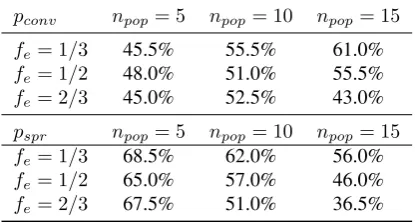
MACS was tuned on the three-impulse case. In particular, the crowding factorwc, the thresholdρtol and the convergenceρmin were kept constant to 1e-5, which is below the required local convergence accuracy, whilefeandnpopwere changed. A value of 1e-5 is expected to provide good local convergence and good density of the samples
belonging to the Pareto front. Table 5 reports the value of performance indexespconv andpsprover 200 runs of MACS with different settings. The indexpsprand the index
pconv have different, almost opposite, trends. However, it was decided to select the setting that provides the best convergence,i.e. npop = 15andfe= 1/3. This setting will be used for all the tests in this paper.
individualistic moves and local archive, denoted asno localin the tables, and one with
no attraction towards the global archiveAg, denoted asno attin the tables. Only these two variants are tested on these cases as they displayed the most significant impact in
the previous standard test cases and more importantly were designed specifically to
improve performances.
NSGA-II, PAES, MOPSO and MTS were tuned as well on the three-impulse case. In
particular, for NSGA-II the best result was obtained for 150 individuals and can be
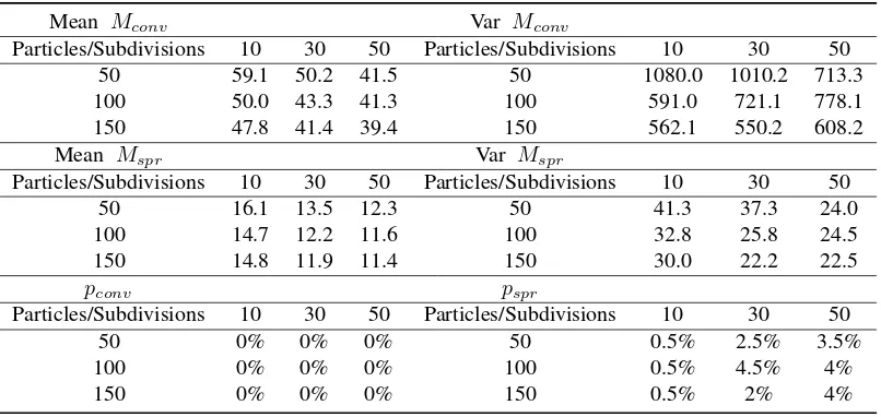
found in Table 6. A similar result could be obtained for MOPSO, see Table 7. For
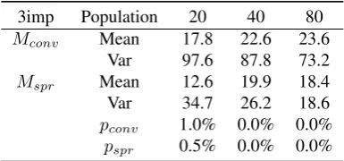
MTS only the population was changed while the number of individuals performing
local moves was kept constant to 5. The results of the tuning of MTS can be found in
Table 9. For the tuning of PAES the results can be found in Table 8.
All the parameters tuned in the three impulse case were kept constant except for the
population size of NSGA-II and MOPSO. The size of the population of NSGA-II and
MOPSO was set to 100 and 40 respectively on the two impulse case and was increased
with the number of function evaluations in the Cassini case. In particular for
NSGA-II the following ratios between population size and number of function evaluations
was used: 272/180000, 353/300000, 500/600000. For MOPSO the following ratios
between population size and number of function evaluations was used: 224/180000,
447/300000, 665/600000. This might not be the best way to set the population size for
these two algorithms but it is the one that provided better performance in these tests.
Note that the size of the global archive for MACS was constrained to be lower than
the size of the population of NSGA-II, in order to avoid any bias in the computation of
Mspr.
The performance of all the algorithms on the Cassini case can be found in Table 12 for
a variable number of function evaluations.
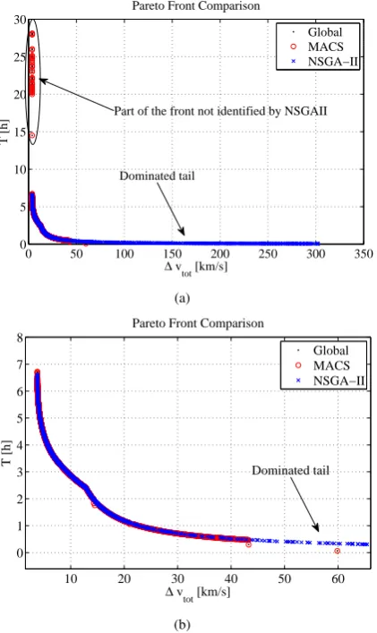
Figure 2: Three-impulse test case: a) Complete Pareto front, b) close-up of the Pareto fronts
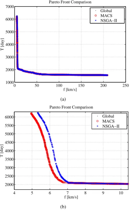
Figure 3: Cassini test case: a) Complete Pareto front, b) close-up of the Pareto fronts
For the three-impulse case, MACS was able to identify an extended Pareto front (see
Fig.2(a) and Fig. 2(b) where all the non-dominated solutions from all the 200 runs are
compared to the global front), compared to the results in [7]. The gap in the Pareto
front is probably due to a limited spreading of the solutions in that region. Note the
cusp due the transition between the condition in which 2-impulse solutions are optimal
and the condition in which 3-impulse solutions are optimal.
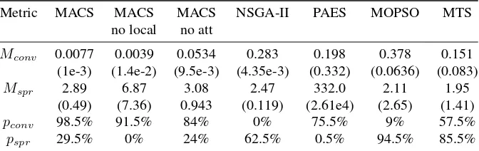
Table 11 summarizes the results of all the tested algorithms on the two-impulse case.
The average value of the performance metrics is reported with, in brackets, the
associ-ated variance over 200 runs. The two-impulse case is quite easy and all the algorithms
have no problems identifying the front. However, MACS displays a better convergence
than the other algorithms while the spreading of MOPSO and MTS is superior to the
one of MACS.
The three-impulse case is instead more problematic (see Table 10). NSGA-II is not
able to converge to the upper-left part of the front and therefore the convergence is 0
and the spreading is comparable to the one of MACS. All the other algorithms perform
poorly with a value of almost 0 for the performance indexes. This is mainly due to the
fact that no one can identify the vertical part of the front.
Note that the long tail identified by NSGA-II is actually dominated by two points
be-longing to the global front (see 2(b)).
Table 12 reports the statistics for the Cassini problem. On top of the performance of the
three variants tested on the other two problems, the table reports also the result for 10
agents andfe= 5. For all numbers of function evaluations MACS has better spreading than II because II converges to a local Pareto front. Nonetheless
NSGA-II displays a more regular behavior and a better convergence for low number of function
evaluations although it never reaches the best front. The Pareto fronts are represented
in Fig. 3(a) and Fig. 3(b) (even in this case the figures represent all the non-dominated
is the best known solution for the single objective version of this problem (see [9]). All
the other algorithms perform quite poorly on this case.
Of all the variants of MACS tested on these problems the full complete one is
per-forming the best. As expected, in all three cases, removing the individualistic moves
severely penalizes both convergence and spreading. It is interesting to note that
re-moving the attraction towards the global front is also comparatively bad. On the two
impulse case it does not impact the spreading but reduces the convergence, while on
the Cassini case, it reduces mean and variance but the success rates are zero. The
ob-servable reason is that MACS converges slower but more uniformly to a local Pareto
front.
Finally, it should be noted that mean and variance seem not to capture the actual
per-formance of the algorithms. In particular they do not capture the ability to identify the
whole Pareto front as the success rates instead do.
Table 6: NSGAII tuning on the 3-impulse case
Table 7: PAES tuning on the 3-impulse case
5. CONCLUSIONS
In this paper we presented a hybrid evolutionary algorithm for multiobjective
opti-mization problems. The effectiveness of the hybrid algorithm, implemented in a code
called MACS, was demonstrated at first on a set of standard problems and then its
per-formance was compared against NSGA-II, PAES, MOPSO and MTS on three space
trajectory design problems. The results are encouraging as, for the same computational
effort (measured in number of function evaluations, MACS was converging more
accu-Table 8: MOPSO tuning on the 3-impulse case.
rately than NSGA-II on the two-impulse case and managed to find a previously
undis-covered part of the Pareto front of the three-impulse case. As a consequence, on the
three-impulse case, MACS, has better performance metrics than the other algorithms.
On the Cassini case NSGA-II appears to converge better to some parts of the front
al-though MACS yielded solutions with better f and identifies once more a part of the front that NSGA-II cannot attain. PAES and MTS do not perform well on the Cassini
case, while MOPSO converges well locally but, with the settings employed in this
study, yielded a very poor spreading.
From the experimental tests in this paper we can argue that the following mechanisms
seem to be particularly effective: the use of individual local actions with a local archive
as they allow the individuals to move towards and within the Pareto set; the use of an
attraction mechanism as it accelerates convergence.
Finally it should be noted that all the algorithms tested in this study use the Pareto
dominance as selection criterion. Different criteria, like the decomposition in scalar
subproblems, can be equality implemented in MACS, without disrupting its working
principles, and lead to different performance results.
ACKNOWLEDGEMENTS
The authors would like to thank Dr. Edmondo Minisci and Dr. Guilio Avanzini for the
two and three impulse cases and the helpful advice.
REFERENCES
[1] V. Coverstone-Caroll, J.W. Hartmann, and W.M. Mason. Optimal multi-objective
low-thrust spacecraft trajectories. Computer Methods in Applied Mechanics and
Engineering, 186:387–402, 2000.
[2] B. Dachwald. Optimization of interplanetary solar sailcraft trajectories using
evo-lutionary neurocontrol.Journal of Guidance, and Dynamics, February 2004.
[3] S. Lee, P. von Allmen, W. Fink, A.E. Petropoulos, and R.J. Terrile.
Proceedings of the Genetic and Evolutionary Computation Conference (GECCO
2005), Washington DC, USA, June 25–29 2005.
[4] O. Sch¨utze, M. M. Vasile, and C.A. Coello Coello. Approximate solutions in
space mission design. InParallel Problem Solving from Nature (PPSN 2008),
Dortmund, Germany, September 13–17 2008.
[5] O. Sch¨utze, M. Vasile, O. Junge, M. Dellnitz, and D. Izzo. Designing optimal
low-thrust gravity-assist trajectories using space pruning and a multi-objective
approach.Engineering Optimization, 41(2), February 2009.
[6] M. Dellnitz, S. Ober-Blbaum, M. Post, O. Schtze, and Bianca Thiere. A
multi-objective approach to the design of low thrust space trajectories using optimal
control.Celestial Mechanics and Dynamical Astronomy, 105(1), February 2009.
[7] E. Minisci and G. Avanzini. Optimisation of orbit transfer manoeuvres as a
test benchmark for evolutionary algorithms. InProceedings of the 2009 IEEE
Congress on Evolutionary Computation (CEC2009), Trondheim, Norway, May
2009.
[8] M. Vasile. A behavioral-based meta-heuristic for robust global trajectory
opti-mization. InProceedings of the 2007 IEEE Congress on Evolutionary
Computa-tion (CEC2007), Singapore, September 2007.
[9] M. Vasile and M. Locatelli. A hybrid multiagent approach for global trajectory
optimization.Journal of Global Optimization, 44(4):461–479, August. 2009.
[10] Oliver Sch¨utze, Adriana Lara, Gustavo Sanchez, and Carlos A. Coello Coello.
HCS: A new local search strategy for memetic multi-objective evolutionary
algo-rithms. IEEE Transactions on Evolutionary Computation (to appear), 2010.
[11] Q. Zhang and H. Li. Moea/d: A multiobjective evolutionary algorithm based on
decomposition.IEEE Transactions on Evolutionary Computation, 11(6),
[12] K.V. Price, R.M. Storn, and J.A. Lampinen. Differential Evolution. A Practical
Approach to Global Optimization. Natural Computing Series. Springer, 2005.
[13] M. Vasile and F. Zuiani. A hybrid multiobjective optimization algorithm applied
to space trajectory optimization. InProceedings of the IEEE International
Con-ference on Evolutionary Computation, Barcelona, Spain, July 2010.
[14] K. A. Deb, A. Pratap, and T. Meyarivan. Fast elitist multi-objective genetic
algo-rithm: Nga-ii. Kangal report no. 200001, KanGAL, 2000.
[15] C. Coello and M. Lechuga. Mopso: A proposal for multiple objective particle
swarm optimization. Technical report evocinv-01-2001., CINVESTAV. Instituto
Politecnico Nacional. Col. San Pedro Zacatenco. Mexico., 2001.
[16] J.D. Knowles and D.W. Corne. The pareto archived evolution strategy : A new
baseline algorithm for pareto multiobjective optimisation. InProceedings of the
IEEE International Conference on Evolutionary Computation, Washington DC,
US, 1999.
[17] Lin-Yu Tseng and Chun Chen. Multiple trajectory search for multiobjective
opti-mization. InProceedings of the IEEE International Conference on Evolutionary
Computation, Singapore, 25-28 September 2007.
[18] D.A. Van Veldhuizen and G.B. Lamont. Evolutionary computation and
conver-gence to a pareto front. InLate Breaking papers at the Genetic Programming,
1998.
[19] M. Vasile, E. Minisci, and M. Locatelli. On testing global optimization algorithms
for space trajectory design. InAIAA/AAS Astrodynamic Specialists Conference,
Honolulu, Hawaii, USA, Aug 2008.
[20] G. Avanzini. A simple lambert algorithm. Journal of Guidance, Control, and
Dynamics, 31(6):1587–1594, Nov.–Dec. 2008.
[21] R. Battin. An Introduction to the Mathematics and Methods of Astrodynamics.
[22] D. R. Myatt, V.M. Becerra, S.J. Nasuto, and J.M. Bishop. Global
opti-mization tools for mission analysis and design. Final rept. esa ariadna itt
Table 10: Summary of metrics Mconv and Mspr, and associated performance indexespconvandpspr, on the three impulse test cases.
Table 11: MetricsMconv andMspr, and associated performance indexespconv andpspr, on the two impulse test cases.
NOMENCLATURE
Ag global archive
Al local archive
aT semimajor axis
D search space
eT eccentricity
f cost function
fe fraction of the population doing local moves
Id dominance index
Mconv convergence metrics
Mspr spreading metrics
Nρ neighborhood of solutionx
Ne maximum number of allowed function evaluations
neval number of function evaluations
npop population size
Pi i-th planet
Pk population at generationk
pconv percentage of success on convergence
pspr percentage of success on spreading
r random number
rp pericentre radius
rpmin minimum pericentre radius
S selection function
s resource index
T transfer time
t0 departure time
ti manoeuvre time
tf final time
u variation of the solutionx
X Pareto optimal set
x solution vector
y mutate individual
wc tolerance on the maximum allowable crowding
Greek symbols
∆v variation of velocity
ρ size of the neighborhoodNρ
µE gravity constant
LIST OF TABLES
Table 1: Multiobjective test functions
Scha f2= (x−5)2
x∈[−5,10] f1=
−x if x≤1
−2 +x if 1< x <3 4−x if 3< x≤4
−4 +x if x >4
Deb f1=x1
x1, x2∈[0,1] f2= (1 + 10x2) [
1− (
x1
1+10x2
)α −
α= 2;q= 4 x1
1+10x2 sin(2πqx1)
]
Deb2 f1=x1
x1∈[0,1] f2=g(x1, x2)h(x1, x2);g(x1, x2) = 11 +x2
2−10 cos(2πx2) x2∈[−30,30] h(x1, x2) =
{ 1−√f1
g iff1≤g
0 otherwise
ZDT2 g= 1 +n−91∑ni=2xi
xi∈[0,1]; h= 1−(fg1)2
i= 1, . . . , n f1=x1;f2=gh n= 30
ZDT4 g= 1 + 10(n−1) +∑ni=2[x2i −10 cos(2πqxi)];
x1∈[0,1]; h= 1− √
f1
g
xi∈[−5,5]; f1=x1;f2=gh
i= 2, . . . , n n= 10
ZDT6 g= 1 + 94
√∑n
i=2xi
n−1 xi∈[0,1]; h= 1−(fg1)2
i= 1, . . . , n f1= 1−exp(−4x1) sin6(6πx1);f2=gh n= 10
Table 2: Comparison of the average Euclidean distances between 500 uniformly space points on the optimal Pareto front for various optimization algorithms: smaller dimension test problems.
Approach Deb2 Scha Deb
MACS 1.542e-3 3.257e-3 7.379e-4
(5.19e-4) (5.61e-4) (6.36e-5)
NSGA-II 0.094644 0.001594 0.002536
(0.117608) (0.000122) (0.000138)
PAES 0.259664 0.070003 0.002881
(0.573286) (0.158081) (0.00213)
MOPSO 0.0011611 0.00147396 0.002057
[image:34.595.179.414.592.710.2]Table 3: Comparison of the average Euclidean distances between 500 uniformly space points on the optimal Pareto front for various optimization algorithms: larger dimension test problems.
Approach ZDT2 ZDT4 ZDT6
MACS 9.0896e-4 0.0061 0.0026
(4.0862e-5) (0.0133) (0.0053)
NSGA-II 0.000824 0.513053 0.296564
(<1e-5) (0.118460) (0.013135)
PAES 0.126276 0.854816 0.085469
[image:35.595.134.464.360.504.2](0.036877) (0.527238) (0.006644)
Table 4: Comparison of different versions of MACS.
Approach Metric ZDT2 ZDT4 ZDT6 Scha Deb Deb2
MACS pconv 83.5% 75% 77% 73% 70.5% 60%
pspr 22.5% 28% 58.5% 38.5% 83% 67.5 %
MACS pconv 14% 0% 45% 0.5% 72.5% 11%
no local pspr 1% 0% 34% 0% 4% 15%
MACS pconv 84% 22% 78% 37% 92% 21%
ρ= 1 pspr 22% 7% 63% 0% 54% 38%
MACS pconv 56% 42% 57% 78% 85% 42%
ρ= 0.1 pspr 5% 15% 61% 88% 94.5% 74%
MACS pconv 21% 0.5% 14.5% 0.5% 88.5% 0%
no attraction pspr 0% 0.5% 78.5% 0% 0% 0%
Table 5: Indexespconvandpspr for different settings of MACS on the 3-impulse case
pconv npop= 5 npop= 10 npop= 15
fe= 1/3 45.5% 55.5% 61.0%
fe= 1/2 48.0% 51.0% 55.5%
fe= 2/3 45.0% 52.5% 43.0%
pspr npop= 5 npop= 10 npop= 15
fe= 1/3 68.5% 62.0% 56.0%
fe= 1/2 65.0% 57.0% 46.0%
[image:35.595.193.401.589.700.2]Table 6: NSGAII tuning on the 3-impulse case
Mean Mconv Var Mconv
ηc/ηm 5 25 50 ηc/ηm 5 25 50
5 36.1 38.3 43.0 5 201.0 202.0 185.0
10 32.3 39.4 40.6 10 182.0 172.0 182.0
20 31.7 39.6 42.5 20 175.0 183.0 169.0
Mean Mspr Var Mspr
ηc/ηm 5 25 50 ηc/ηm 5 25 50
5 6.77 7.24 8.08 5 9.97 9.47 7.25
10 5.91 7.50 7.81 10 9.74 8.68 8.34
20 5.78 7.50 8.16 20 9.75 8.53 8.04
pconv pspr
ηc/ηm 5 25 50 ηc/ηm 5 25 50
5 0.0% 0.0% 0.0% 5 44.8% 37.7% 23.4%
10 0.0% 0.0% 0.0% 10 57.8% 33.1% 29.2%
20 0.0% 0.0% 0.0% 20 61.0% 32.5% 24.7%
Table 7: MOPSO tuning on the 3-impulse case.
Mean Mconv Var Mconv
Particles/Subdivisions 10 30 50 Particles/Subdivisions 10 30 50
50 59.1 50.2 41.5 50 1080.0 1010.2 713.3
100 50.0 43.3 41.3 100 591.0 721.1 778.1
150 47.8 41.4 39.4 150 562.1 550.2 608.2
Mean Mspr Var Mspr
Particles/Subdivisions 10 30 50 Particles/Subdivisions 10 30 50
50 16.1 13.5 12.3 50 41.3 37.3 24.0
100 14.7 12.2 11.6 100 32.8 25.8 24.5
150 14.8 11.9 11.4 150 30.0 22.2 22.5
pconv pspr
Particles/Subdivisions 10 30 50 Particles/Subdivisions 10 30 50
50 0% 0% 0% 50 0.5% 2.5% 3.5%
100 0% 0% 0% 100 0.5% 4.5% 4%
[image:36.595.125.528.490.681.2]Table 8: PAES tuning on the 3-impulse case
Mean Mconv Var Mconv
Subdivisions/Mutation 0.6 0.8 0.9 Subdivisions/Mutation 0.6 0.8 0.9
1 53.7 70.6 70.2 1 525.0 275.0 297.0
2 52.8 70.2 70.0 2 479.0 266.0 305.0
4 53.0 70.2 70.1 4 453.0 266.0 311.0
Mean Mspr Var Mspr
Subdivisions/Mutation 0.6 0.8 0.9 Subdivisions/Mutation 0.6 0.8 0.9
1 14.2 27.7 36.7 1 20.0 14.3 17.3
2 13.6 27.6 36.6 2 17.5 14.6 16.8
4 13.8 27.7 36.6 4 17.2 15.8 17.0
pconv pspr
Subdivisions/Mutation 0.6 0.8 0.9 Subdivisions/Mutation 0.6 0.8 0.9
1 0.0% 0.0% 0.0% 1 0.0% 0.0% 0.0%
2 0.0% 0.0% 0.0% 2 0.0% 0.0% 0.0%
[image:37.595.200.393.424.514.2]4 0.0% 0.0% 0.0% 4 0.0% 0.0% 0.0%
Table 9: MTS tuning on the 3-impulse
3imp Population 20 40 80
Mconv Mean 17.8 22.6 23.6
Var 97.6 87.8 73.2
Mspr Mean 12.6 19.9 18.4
Var 34.7 26.2 18.6
pconv 1.0% 0.0% 0.0%
pspr 0.5% 0.0% 0.0%
Table 10: Summary of metrics Mconv and Mspr, and associated performance indexespconvandpspr, on the three impulse test cases.
Metric MACS MACS MACS NSGA-II PAES MOPSO MTS
no local no att
Mconv 5.53 7.58 154.7 31.7 53.0 39.4 17.8
(15.1) (26.3) (235.0) (175.0) (453.0) (608.1) (97.6)
Mspr 5.25 6.03 9.16 5.78 13.8 11.4 12.6
(3.73) (3.95) (2.07) (9.75) (17.2) (22.5) (34.7)
pconv 61.0% 40.5% 0.0% 0.0% 0.0% 0% 1.0%
[image:37.595.135.459.596.703.2]Table 11: MetricsMconv andMspr, and associated performance indexespconv andpspr, on the two impulse test cases.
Metric MACS MACS MACS NSGA-II PAES MOPSO MTS
no local no att
Mconv 0.0077 0.0039 0.0534 0.283 0.198 0.378 0.151
(1e-3) (1.4e-2) (9.5e-3) (4.35e-3) (0.332) (0.0636) (0.083)
Mspr 2.89 6.87 3.08 2.47 332.0 2.11 1.95
(0.49) (7.36) 0.943 (0.119) (2.61e4) (2.65) (1.41)
pconv 98.5% 91.5% 84% 0% 75.5% 9% 57.5%