High performance microfluidic rectifiers for viscoelastic fluid flow

Sousa, P.C. and Pinho, F.T. and Oliveira, Monica and Alves, M.A. (2012)

High performance microfluidic rectifiers for viscoelastic fluid flow. RSC

Advances, 2 (3). pp. 920-929. ISSN 2046-2069 ,

http://dx.doi.org/10.1039/CIRA00803J

This version is available at https://strathprints.strath.ac.uk/41334/

Strathprints

is designed to allow users to access the research output of the University of

Strathclyde. Unless otherwise explicitly stated on the manuscript, Copyright © and Moral Rights

for the papers on this site are retained by the individual authors and/or other copyright owners.

Please check the manuscript for details of any other licences that may have been applied. You

may not engage in further distribution of the material for any profitmaking activities or any

commercial gain. You may freely distribute both the url (

https://strathprints.strath.ac.uk/

) and the

content of this paper for research or private study, educational, or not-for-profit purposes without

prior permission or charge.

Any correspondence concerning this service should be sent to the Strathprints administrator:

[email protected]

The Strathprints institutional repository (https://strathprints.strath.ac.uk) is a digital archive of University of Strathclyde research outputs. It has been developed to disseminate open access research outputs, expose data about those outputs, and enable the

;

_{High performance microfluidic rectifiers for viscoelastic fluid flow}

Patrı´cia C. Sousa,

Fernando T. Pinho,

Mo´nica S. N. Oliveira

and Manuel A. Alves

*

Received 27th September 2011, Accepted 30th September 2011

DOI: 10.1039/c1ra00803j

The flow of Newtonian and non-Newtonian fluids within microfluidic rectifiers with a hyperbolic shape was investigated to assess the effect of the bounding walls on the diodicity of the microfluidic device and achieve high flow anisotropy. Three microchannels were used, with different depths and the same geometrical configuration, which creates a strong extensional flow and generates high anisotropic flow resistance between the two flow directions. The Newtonian fluid, de-ionized water, was used as a reference fluid. The viscoelastic fluid used was an aqueous solution of polyethylene oxide (0.1% w/w) with high molecular weight. The flow patterns were visualized using streak photography and the velocity field was investigated using micro-particle image velocimetry. Moreover, pressure drop measurements were performed in order to compare the diodicity achieved in the microfluidic rectifiers. For the Newtonian fluid flow, the experimental results are compared with numerical predictions obtained using a finite-volume method and good agreement was found between both. For the viscoelastic fluid, significant anisotropic flow resistance can be achieved. The effect of the bounding walls is analysed and found to be qualitatively similar for all microchannels. Nevertheless, in quantitative terms, the diodicity is enhanced when the wall effect is reduced,i.e.when the channels are deeper. A maximum diodicity above six was found for the deeper channel, a value well beyond those previously reported.

1. Introduction

Microfluidic devices are systems which operate with small amounts of fluids and have integrated channels, whose dimen-sions are of the order of tens to hundreds of microns. One current challenge of engineering science is to scale-down (process intensification) in order to achieve integrated and portable ‘‘lab-on-a-chip’’ tools able to operate with high resolution and sensitivity, short analysis time, low cost and reduced volumes of reagents and waste.1Microfluidic technology is applied across fields: in biology for cellular analysis or DNA separation; in medicine for clinical diagnostics; in chemistry to undertake chemical reactions.2–5

The small length scales that characterize these microsystems lead typically to low Reynolds numbers (Re) and consequently laminar flow conditions. Furthermore, surfaces forces, which are often negligible in flows at the macroscale, may become significant in microfluidics due to the strong intermolecular forces.6The fluids of interest in such lab-on-a-chip applications have often non-Newtonian rheological behaviour, as for example

saliva,7 blood,8 several suspensions or other fluids containing small amounts of polymers.9,10

The non-linear rheological properties of these fluids result in complex flow phenomena, which need to be better understood in order to optimize the design of microfluidic devices.

Viscoelastic fluid flow is prone to instabilities, which in microfluidics are often purely elastic in nature as inertial effects are small. These purely elastic instabilities, as documented in Mulleret al.11_{and Larsonet al.}12_{for Taylor-Couette flow, occur}

above a critical Deborah number (De) and result from the combination of curved streamlines and development of large normal stresses. Subsequently, Pakdel and McKinley13proposed a criterion to predict the critical conditions for the onset of purely elastic instabilities.

Utilizing a microfluidic cross-slot geometry, Arratia et al.14

observed experimentally that a viscoelastic fluid under creeping flow conditions can undergo different types of instabilities. These authors reported the onset of a first instability, in which the flow becomes asymmetric but remains steady, followed by a second instability, in which the flow becomes unsteady, with the amplitude of oscillation increasing with the flow rate. Subsequently, Poole et al.15demonstrated that the steady asymmetry observed in the cross-slot geometry can be predicted numerically for creeping flow conditions, using the simplest differential viscoelastic model, the upper-convected Maxwell (UCM) model. Broad attention has been paid recently to geometries in which viscoelastic effects emerge in highly elongational fields, such as the cross-slot,16 T-shaped geometries17and flow-focusing devices.18

a

Departamento de Engenharia Quı´mica, CEFT, Faculdade de Engenharia da Universidade do Porto, Rua Dr Roberto Frias, 4200-465, Porto, Portugal. E-mail: [email protected] Fax +351 225081449; Tel: +351 225081680

b_{Departamento de Engenharia Mecaˆnica, CEFT, Faculdade de Engenharia} da Universidade do Porto, Rua Dr Roberto Frias, 4200-465, Porto, Portugal.

1

5

10

15

20

25

30

35

40

45

50

55

59

1

5

10

15

20

25

30

35

40

45

50

55

59

RSC Advances

Dynamic Article Links

Cite this: DOI: 10.1039/c1ra00803j

www.rsc.org/advances

PAPER

P

R

O

O

Elastic instabilities can be useful to promote mixing at low Reynolds number flows.19 _{In fact, purely elastic instabilities}

stimulate a disordered state of the flow brought about by elastic stresses even at vanishingly smallRe, giving rise to the concept of elastic turbulence.20,21 With the fluid motion occurring over a wide range of temporal and spatial scales, elastic turbulence generates high flow resistance and increases the rate of mixing.22 Taking advantage of elastic nonlinearities, Groisman and co-workers23,24 developed several ingenious microfluidic devices which operate as control and memory elements. These authors exploited the viscoelastic rheological properties of dilute poly-meric fluids and found that increasing the applied pressure gradient lead to complex flow behaviour, due to the differences between coil stretching and relaxation, and consequently the variation of the flow rate was found to be small for a wide range of applied pressures.25A microfluidic rectifier with no moving parts was also developed, making use of the nonlinearities brought about by elastic stresses in viscoelastic fluid flow.24 In the proposed microfluidic device, consisting of a series of triangular cavities, the non-Newtonian fluid experiences a different deformation history when flowing in the two possible flow directions, leading to a significant anisotropic flow resistance. The development of efficient flow rectifiers is an important area of research in microfluidics, namely to be used in the development of piezoelectric-driven micropumps. The technology of microscale pumping has been the aim of several investigations with applications as diverse as drug delivery systems, fuel delivery in engines and cooling in micro-electronics.25 However, despite the interest of non-Newtonian fluid flows in microfluidics, in these studies, the flow of Newtonian fluids has been much more frequently investigated and studies of microfluidic rectifiers using viscoelastic fluids are still scarce.24,26,27

With the aim of designing more efficient microfluidic rectifiers for viscoelastic fluids that are able to operate even under creeping flow conditions, we presented previously a comparison between the efficiency of distinct geometries, namely the

triangular nozzle/diffuser rectifier proposed in the literature and a new rectifier based on hyperbolic-shaped elements.27 _A

detailed investigation, in terms of pressure drop measurements and visualizations of the flow patterns for different viscoelastic fluids as well as for a Newtonian reference fluid, was carried out. In that work, hyperbolic-shaped geometries were chosen based on the work of Oliveiraet al.28in order to generate a quasi-ideal extensional flow and the device with a Hencky straineH= 2 was

identified to exhibit the highest diodicity. Additionally, the importance of wall effects imposed by the shallow depth of the microchannels and its influence on the diodicity arose as an important topic for further research. Therefore, here, we investigate the effect of channel depth on the diodicity using the most efficient hyperbolic shaped microfluidic rectifier presented earlier.27For this purpose, we use three microchannels with different depths,h= 46 mm, 88mm and 120mm. Pressure drop measurements in addition to flow visualization and micro-particle image velocimetry (mPIV) measurements were carried out for a wide range of flow rates. The non-Newtonian fluid used here is an aqueous solution of a high molecular weight polyethylene oxide (PEO), with molecular weight Mw = 8 6

106g mol21_{, which presented the highest rectification effect of all}

the fluids tested previously.27Moreover, the flow of a Newtonian fluid (de-ionized water) is also investigated in order to validate the experimental techniques and to be used as reference.

2. Experimental

2.1 Experimental techniques

The three microchannels used in the experiments were designed to have the same generic geometrical shape but different depths (h).

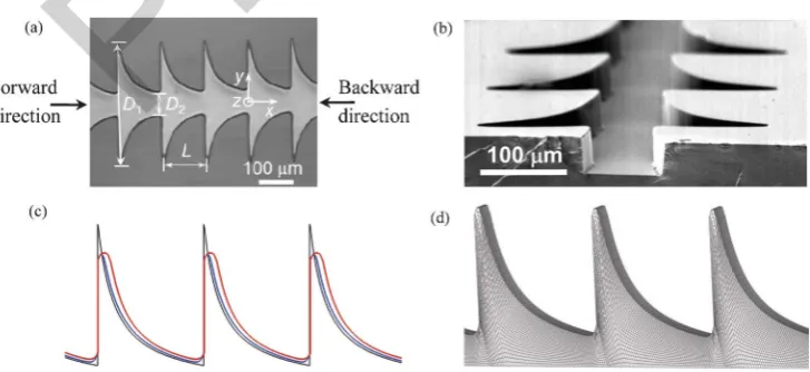
The devices, fabricated in polydimethylsiloxane (PDMS) using standard soft-lithography,29include two inlets/outlets located at the extremes of the channels and two pressure taps on each side of the test section of the microgeometry. In Fig. 1(a) we show an optical transmission microscope image of a typical microchannel

Fig. 1 (a) Optical micrograph of the hyperbolic microfluidic rectifier A (h= 46mm). Microchannels B and C have the same geometrical shape but have depths of 88mm and 120mm, respectively. (b) SEM image illustrating the verticality of the walls of microchannel A. Only part of the microchannels is shown. (c) Comparison between the designed shape of the microchannel (thin black line), the real shape of the microchannel A (h= 46mm, blue line) and the real shape of microchannels B and C with 88mm and 120mm in depth, respectively (red line). Note that the shape of microchannels B and C are similar. (d) Zoomed view of the coarse mesh used in the numerical simulation of the Newtonian fluid flow in microchannel A.

1

5

10

15

20

25

30

35

40

45

50

55

59

1

5

10

15

20

25

30

35

40

45

50

55

59

P

R

O

O

used in the experiments. A scanning electron microscopy (SEM) image of the 46mm deep microchannel is also shown in Fig. 1(b) to illustrate the well-defined and quasi-vertical walls of the PDMS microchannels. The general hyperbolic function that was used to describe the shape of the channels isy=¡a/(1 +b x), with a = 200 mm and b= 0.05 mm21_{;x is the axial position}

(0 ¡ x/mm ¡ L), where L is the length of each hyperbolic element (L= 128mm). Each microfluidic diode is composed of 42 repetitive hyperbolic elements. The chrome mask used in the manufacturing process follows closely this hyperbolic shape and was used to make the moulds from which the channels were produced, which in principle would only differ in depth. However, the actual moulds are slightly different due to inaccuracies inherent to the photolithography fabrication procedure and this results in small differences in the shape of the final PDMS channels as shown in Fig. 1(c). The corresponding characteristic dimensions of the channels are given in Table 1, including the total Hencky strain (eH), defined aseH= ln(D1/D2).

The shape of the microchannels follows closely the following curves:

Channel A (h= 46mm)

y=mm

j j~153:6z2:3

ffiffiffiffiffiffiffiffiffiffiffiffiffiffiffiffiffiffiffiffiffiffiffiffiffi 42_{(x{4)2

q

0vx=mmƒ7:7

y=mm

j j~ 220

1z0:052xz15e

(x{128)=3 _{7:7vx=mmƒ128}

8 > > > < > > > : (1)

Channel B (h= 88mm) and channel C (h= 120mm)

y=mm

j j~155:5z

ffiffiffiffiffiffiffiffiffiffiffiffiffiffiffiffiffiffiffiffiffiffiffiffiffiffiffiffiffiffiffiffi 7:52_{(x{7:5)2

q

0vx=mmƒ14:9

y=mm

j j~ 380

1z0:097x{9:1|10{5_x2z10e (x{128)=4

14:9vx=mmƒ128 8 > > > > > > > < > > > > > > > : (2)

The configuration of the experimental set-up used in this work is identical to that employed in a previous work.27 Flow is imposed by means of a syringe pump (PHD2000, Harvard Apparatus), used to feed the fluid to the channels and control the volumetric flow rate.

For pressure drop measurements, the pressure taps in the microchannel were connected to a pressure transducer (Honeywell, model 26PC series) in order to measure the differential pressure drop inside the test section. A 12 V DC power supply (Lascar electronics, PSU 206) was used to power the pressure sensors that were also connected to a computer,via

a data acquisition card (NI USB-6218, National Instruments). The output data was recorded using LabView v7.1. The pressure sensors were calibrated using a static column of water or using a compressed air line depending on the pressure range. A detailed description can be found in Sousaet al.27

Visualizations of the flow patterns and measurements of the velocity field were performed at the centreplane of the micro-channel i.e. at mid-distance between top and bottom planar bounding walls. The imaging experimental set-up is composed of an inverted epi-fluorescence microscope (DMI 5000M, Leica Microsystems GmbH) equipped with a filter cube (Leica Microsystems GmbH, excitation filter BP 530–545 nm, dichroic 565 nm and barrier filter 610–675 nm) as well as with a light source, objective and digital camera appropriate for each optical technique used.

For visualizations of the flow patterns, we employed streak photography. For this, the light source used was a 100 W mercury lamp. The fluids were seeded with 1 mm fluorescent tracer particles (Nile Red, Molecular Probes, Invitrogen, Ex/Em: 520/580 nm) and the streak images were captured through a 106(NA = 0.25) objective lens using a CCD camera (DFC350 FX, Leica Microsystems GmbH).

For micro-particle image velocimetry measurements, the fluorescent particles used are 0.5 mm in diameter and the light source was a double-pulsed 532 nm Nd:YAG laser (Dual Power 65–15, Dantec Dynamics). Images were captured using a 206 (NA = 0.4) microscope objective and a CCD digital camera (Flow Sense 4M, Dantec Dynamics), with a resolution of 20486 2048 pixels and running on double frame mode. The time interval between pulses was adjusted so that the displacement of the particles between the two consecutive frames was about 25% of the width of the interrogation area. Interrogation areas of 64632 pixels, with a 50% overlap were used to create the vector maps. For steady flow, the vector maps were obtained by ensemble averaging 150 pairs of images. On the other hand, for unsteady flow, we present both instantaneous and ensemble-average vector maps obtained from a set of 1000 pairs of images. The depth over which there is a contribution of unfocused particles to the velocity field determined bymPIV is called the total measurement depth,dzm, and can be calculated as the sum

of three different effects: the effect due to diffraction, the effect due to geometrical optics and the effect due to the finite size of the particle,30respectively corresponding to the first, second and third terms on the right-hand-side of Eqn (3):

dzm~

3nl0

(NA)2z 2:16dp

tanh zdp (3)

wherenis the refractive index,l0is the wavelength of the light

(in vacuum), NA is the numerical aperture of the microscope objective anddpis the seeding particle diameter. For the streak

imaging optical set-up, the measurement depth isdzm= 37mm,

whereas for themPIV set-up,dzm= 14mm.

2.2. Fluid rheology

The fluids used in this investigation consist of a Newtonian fluid (de-ionized water) and a non-Newtonian fluid, which is an aqueous solution of a high molecular weight polyethylene oxide

Table 1 Dimensions of the hyperbolic microgeometries and resulting Hencky strain values

Projected (chrome mask) PDMS microchannel

D1

[mm] D2

[mm] eH L [mm]

h [mm]

D1

[mm] D2

[mm] eH

Channel A 400 54 2.0 128 46 326 63 1.64 Channel B 400 54 2.0 128 88 326 70 1.54 Channel C 400 54 2.0 128 120 326 70 1.54

(PEO, Mw = 86106 g mol21, Sigma-Aldrich) at 0.1% (w/w) concentration. The density of the viscoelastic fluid, measured at the reference temperature (T0= 293.2 K), isr= 998 kg m2

3

. The rheological properties of the viscoelastic solution were characterized in steady shear and in uniaxial extension flow and are presented in Sousaet al.,27where a thorough description of the experimental rheological characterization and techniques can be found. Here, only the most relevant results are presented. The characteristic relaxation time of the viscoelastic fluid (l), measured at the reference temperature using a capillary break-up extensional rheometer (CaBER), was found to be 73.9 ms.

Shear rheology measurements were performed on a rotational rheometer (Physica MCR301, Anton Paar) using a cone-plate geometry with 75 mm diameter and 1uangle in the temperature range of 283.2 ¡ _T/K ¡ _{303.2. The flow curves obtained} experimentally were shifted to the reference temperature (T0=

293.2 K) using the time-temperature superposition method in order to obtain the master curve and the temperature influence on the shift factor,aT, generally defined as:31

aT~

g(T)

g(T0)

T0

T

r₀

r (4)

whereg(T0) is the shear viscosity at the reference temperature

T0,g(T) is the shear viscosity at a given temperature Tandr0

and r are the fluid densities at temperatures T0 and T,

respectively.

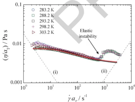
Fig. 2 shows the master curve obtained for the viscoelastic fluid, which was fitted using the simplified form of the single-mode linear Phan-Thien-Tanner (sPTT) single-model32with a solvent contribution. The parameters obtained were: extensibility para-meter,e= 0.04; polymer viscosity coefficient,gP= 0.0045 Pa s;

relaxation time, l = 73.9 ms (determined from CaBER measurements); Newtonian solvent viscosity, gS = 0.003 Pa s.

More details can be found in Sousaet al.27The flow curve was also fitted using the Carreau-Yasuda model,33which is able to

model the fluid shear-thinning behaviour, but not its elasticity:

g=gS+ (g02gS)/[1 + (Lc_) a

](12n)/a_{. The corresponding parameters}

are:g0= 0.0075 Pa s,gS= 0.003 Pa s,L= 0.05 s,n= 0.53 and

a= 1.8. The predictions of both models are shown in Fig. 2, and this information can be useful, for example, for future numerical calculations.

3. Numerical

3.1. Governing equations and numerical method

The Newtonian fluid flow was simulated numerically using a fully-implicit finite-volume method with a time marching pressure-correction algorithm.34 The governing equations that describe an isothermal, laminar and incompressible fluid flow are those of conservation of mass and momentum:

+_?u= 0 (5)

r Lu

L_tzu:+u

~{+_pz+:t (6)

wherepis the pressure and the extra-stress tensor (t) is defined as

the sum of the contribution of a solvent and a polymeric solute (t=ts +tp). Since in this work we will restrict the numerical simulations to Newtonian fluid flows, the polymeric contribution to the extra-stress tensor is null (tp= 0) and the stress-tensor is calculated considering only the solvent contribution:

ts~g(c_) +uz+uT

(7)

where g(c_) can be either constant (Newtonian fluid,g(c_)~g_S) or shear-rate dependent for a generalized Newtonian fluid (GNF), such as the Carreau-Yasuda, in whichg(c_) is a function of the shear rate, defined asc_~ ffiffiffiffiffiffiffiffiffiffiffiffiffiffiffiII(c_)=2

p

, whereII(c_) represents the second invariant of the shear rate tensor,c_~+uz+uT.

In the numerical method, the governing eqn (5) and (6) are integrated in time over a small time step (dt) and in space over the control volumes of the computational mesh. Regarding the accuracy of the calculations, the time derivative is discretized using an implicit first-order Euler scheme, the diffusive terms are discretized using second-order central differences and a high-resolution scheme, CUBISTA35is used for the discretization of the advective terms. More details of the numerical method used can be found in Oliveiraet al.34_{and Alveset al.}35

3.2. Computational meshes and dimensionless numbers

We performed numerical simulations of the Newtonian fluid flowing in the forward and backward flow directions of the hyperbolic shaped rectifier. The meshes used to describe the computational domain are three-dimensional, block-structured and are composed of non-uniform cells. Due to symmetry of the Newtonian fluid flow under steady flow conditions, observed in the experiments, symmetry boundary conditions were imposed at the two centreplanes (x = 0 andz= 0), thus only a quarter of the total domain was used in the numerical simulations. The computational domain consists of two long straight channels that define the inlet and outlet channels and 10 hyperbolic elements which define the test section and have dimensions matching exactly those used in the experiments. As explained previously in Section 2.1, the fabricated microchannels present

Fig. 2 Master curve of the steady shear viscosity for the viscoelastic fluid (symbols) at the reference temperature (T0= 293.2 K). The solid

and the dotted lines represent the fit of the sPTT and Carreau-Yasuda models to the experimental data, respectively. The dashed straight lines represent the minimum measurable shear viscosity determined from 206

the minimum measurable torque of the rheometer (i) and the onset of secondary flow due to Taylor instabilities (ii).

1

5

10

15

20

25

30

35

40

45

50

55

59

1

5

10

15

20

25

30

35

40

45

50

55

59

P

R

O

O

slight differences relative to the idealized hyperbolic shape, due to inaccuracies inherent to the fabrication procedure. As such, the numerical simulations were carried out in the computational domains corresponding to the real geometries described by eqn (1) and(2), rather than the idealized shape printed on the chrome mask [Fig. 1(c)]. We also note that the experimental geometries consist of 42 repeating hyperbolic units, while in the numerical simulations only 10 elements were used in order to reduce the size of the meshes and reduce the computational times. The numerical results confirm that for all flow conditions investi-gated numerically, the flow field in the hyperbolic elements located in the middle of the computational domain is already fully-developed, and therefore using only 10 elements in the numerical simulations is enough to obtain accurate results since the comparisons are made on the basis of dimensionless quantities. A zoomed perspective of the mesh used for the simulations with channel A is illustrated in Fig. 1(d). Moreover, the Newtonian fluid flow in channel A was simulated using another mesh, with higher refinement level. For channel A, mesh M1 has a total of 290 304 cells, while mesh M2 has a total number of 2 322 432 cells, and was created by doubling the number of cells in each direction. For channels B and C, only mesh M1 was used, also consisting of 290 304 cells.

Except for the (inlet/outlet) boundary conditions, the meshes used for the forward and backward flow directions are similar in their characteristics. The inlets and outlets were positioned far from the hyperbolic elements that define the test section allowing fully developed flow conditions to be attained well upstream and downstream of the hyperbolic elements. No-slip boundary conditions were imposed at the solid walls, and at the inlet, a uniform velocity profile was imposed. At the outflow boundary, vanishing streamwise gradients of velocity components are imposed and pressure is linearly extrapolated from the two upstream cells.

Regarding the relevant dimensionless numbers, the aspect ratio of the channel is defined as AR =h/D2. The Newtonian

fluid flow is also characterized using the Reynolds number,Re=

rU2D2/g0, based on the flow characteristics at the contraction

throat, where U2 is the average velocity, D2 is the width [cf.

Fig. 1(a)] andg0is the fluid shear viscosity. For the viscoelastic

fluid flow, the zero-shear rate viscosity (g0=gP+gs) is used in

the definition of the Reynolds number. Additionally, to characterize the viscoelastic fluid flow we use the Deborah number (De), also based on the flow characteristics at the throat: De = lU2/(D2/2). The relaxation time and the shear viscosity

used in computation ofDeandReare evaluated at the tempera-ture of the experiments.

The diodicity, which is used to characterize the rectification effects, is defined as the ratio between the pressure drop in the forward direction, DPForward, and the pressure drop in the

backward direction,DPBackward, at the same flow rate: Di|Q=

DPForward/DPBackward.

4. Results and discussion

4.1. Flow patterns

The Newtonian fluid flow patterns observed in hyperbolic shaped rectifiers, including rectifier A, were discussed in detail in Sousa et al.27 and therefore are not repeated here. For

Newtonian fluid flow through rectifier B and C, the flow patterns observed are qualitatively similar to those in rectifier A and in these three channels the diodicity is nearly unitary for the range of flow rates investigated (i.e.no rectification effects are observed). The flow phenomena observed in the viscoelastic fluid flow through the hyperbolic shaped microfluidic rectifiers A, B and C is qualitatively similar. Streak images obtained in rectifier B (AR= 1.26,h= 88mm) are shown in Fig. 3. At low flow rates, Newtonian-like flow patterns are observed, exhibiting recircula-tions inside the hyperbolic corner for both flow direcrecircula-tions [Fig. 3(a); forward flow in the first row and backward flow in the second row]. Increasing the flow rate, a distinct flow behaviour is found for the two flow directions, as documented previously in Sousa et al.27 For the forward direction, the flow becomes asymmetric and unsteady due to onset of elastic instabilities, and recirculations appear and disappear randomly within the hyperbolic elements [cf. Fig. 3(b) in the first row]. In the previous work with the 46 mm depth microfluidic rectifier, the onset of these purely elastic instabilities was linked to the appearance of rectification effects.27 _{In that work, a nominal}

depth of 50 mm was assumed, but subsequent SEM measure-ments of the microchannels showed that the correct depth is 46mm, as used in this work. Also, in Sousaet al.,27the throat width of the chrome mask was assumed in the calculations while in this work we use the real minimum width of the final PDMS channel, as reported in Table 1. These corrections in the microchannel depth and width lead to an increase of less than 10% inReand a decrease of less than 20% inDevalues relative to those reported in the previous work. The rectification effects emerge (cf. Section 4.3) following the appearance of elastic instabilities [Fig. 3(b) in forward flow]. For the backward flow direction, recirculations are visible near the hyperbolic corners and the flow remains steady as the flow rate (orDe) is increased until a critical De is reached. The critical value for the appearance of elastic instabilities that incite unsteady flow in the backward direction is significantly higher than in the forward flow direction.

In summary, similar flow behaviour is found for the three microfluidic diodes (A, B and C), but the onset of elastic instabilities with the critical Deborah number (Dec) increasing

with the aspect ratio: while for the microchannel A (AR= 0.73, h= 46mm) elastic instabilities are already evident atDec#20 in the forward flow direction, for the microchannel B (AR = 1.26,h= 88mm) and microchannel C (AR= 1.71,h= 120mm), these are delayed toDec#25 andDec#45, respectively.

5. Velocity field

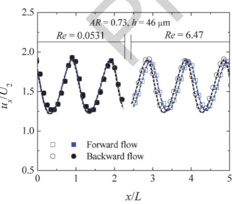
5.1. Newtonian fluid flow—experimental validation

The velocity field of the Newtonian fluid flow in all hyperbolic rectifiers was determined using mPIV for different flow rates. Fig. 4 shows profiles of the dimensionless axial velocity along the centreline of the microfluidic rectifiers with a depth of 46 mm (rectifier A), for both flow directions. Furthermore, the experimental results are compared with the numerical predic-tions using meshes M1 and M2 and the velocity profiles are split in two regions: one region for a lowReand another region for a higherRe. As expected, the velocity profiles along the centreline show a periodic behaviour caused by the geometrical shape of

1

5

10

15

20

25

30

35

40

45

50

55

59

1

5

10

15

20

25

30

35

40

45

50

55

59

P

R

O

O

the microchannel, i.e. the sequence of identical hyperbolic elements composed of contractions. As such, the axial velocity varies from a minimum value at a position near the centre of each element, to a maximum value near the contraction region. As such, the axial velocity varies from a minimum value at a position near the centre of each element, to a maximum value near the contraction region. At low flow rates (lowRe), inertia is negligible and the axial velocity profiles for both flow directions collapse due to the reversibility of Newtonian creeping flows

(left part of Fig. 4). When the flow rate is further increased, differences between the velocity profiles measured for the forward and backward flow directions become noticeable due to inertial effects (right part of Fig. 4) and, it is possible to identify a lag between both profiles. For the forward flow direction inertia pushes the fluid against the hyperbolic (gradual) contraction and the value of the velocity is maximum at the channel throat. On the other hand, for the backward flow direction, the fluid experiences a sudden acceleration when flowing through the abrupt contraction and the maximum value of the axial velocity occurs immediately downstream of the throat. Moreover, it is possible to observe that the amplitude of the velocity oscillation (and consequently the maximum strain rate) in the backward direction is slightly higher than in the forward flow direction. The numerical results presented in Fig. 4 were determined at the centreplane of the computational domain. However, since themPIV measurements take into account not only the focused particles at the centreplane but also unfocused particles at adjacent planes over the whole measure-ment depth,30as described in Section 2.1, a numerical weighted-average velocity in the measurement depth,dzm, was calculated

and a deviation from the centreline velocity field of less than 3% was found for rectifier A. For rectifier C, due to the larger depth, this deviation is significantly lower. Since the imparted difference in velocity is small and considering that the focused particles are responsible for the major contribution to themPIV correlation, the presented numerical axial velocity is taken only at the centreline to compare with the experimental results. As can be seen in Fig. 4, the experimental and numerical results are in good agreement with each other. Moreover, the predictions obtained using meshes M1 and M2 are very similar and deviations between them are smaller than 1%. For this reason, only mesh

Fig. 4 Dimensionless axial velocity along the centreline for Newtonian fluid flow in the hyperbolic rectifier A (AR= 0.73,h= 46mm). Symbols: experimental data; dashed lines: numerical predictions using mesh M1; solid lines: numerical predictions using mesh M2.

Fig. 3 Streak images of the viscoelastic fluid flow in rectifier B (AR= 1.26;h= 88mm) at different flow rates.

1

5

10

15

20

25

30

35

40

45

50

55

59

1

5

10

15

20

25

30

35

40

45

50

55

59

P

R

O

O

M1 was used in the remaining simulations to allow for smaller CPU computational time required to converge the three-dimensional simulations.

5.2. Viscoelastic fluid flow

As shown in Section 4.1, at low flow rates the flow is steady, but above a critical flow rate, elastic instabilities arise and the flow becomes unsteady, initially for the forward direction and then, at significantly higher flow rates, also in the backward flow direction.

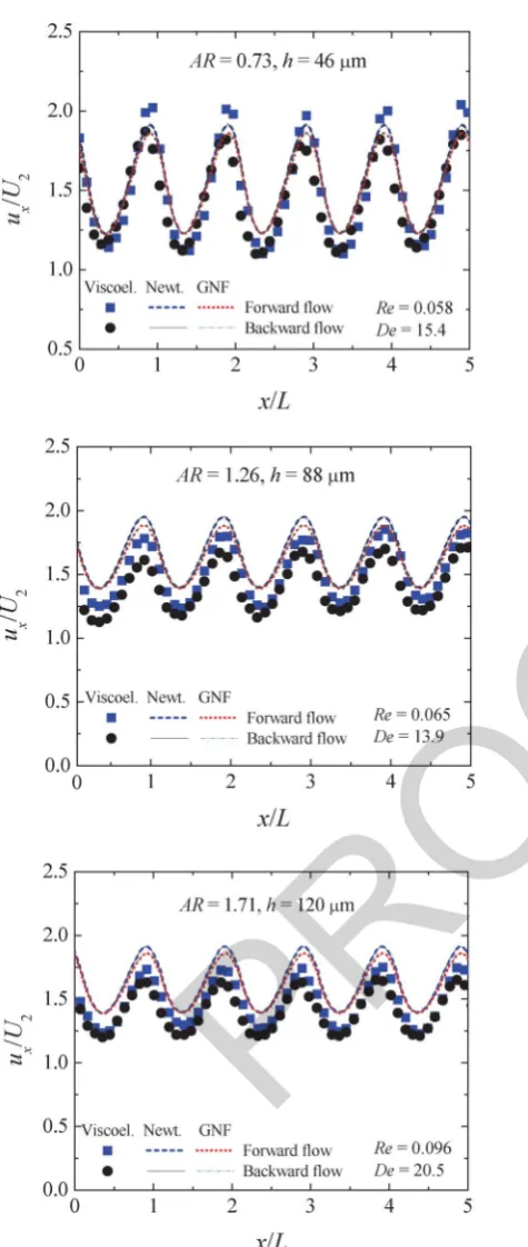
a) Steady flow. Fig. 5 shows the axial velocity profiles measured with the viscoelastic fluid in all microgeometries investigated. The flow rates presented refer to steady flow conditions corresponding to similar flow resistance for both flow directions. Additionally, in Fig. 5 we also show the numerical predictions for a Newtonian fluid and a Carreau-Yasuda model, which exhibits a rheological shear behaviour similar to the viscoelastic fluid used in the experiments (cf.model parameters in Section 2.2), flowing at the same flow rate as the viscoelastic fluid.

The velocity profiles exhibit the expected sinusoidal-like shape, with the experimental profile for the forward direction showing slightly higher amplitude, which is more evident for the cha-nnels with lower depths in contrast to what was observed for Newtonian fluids. Moreover, the forward and backward experimental velocity profiles also show a small lag in the x-direction, mostly due to elastic effects as is clear from Fig. 5(a) where Re is too low for inertial effects to be relevant. Fur-thermore, it is also possible to observe that, for the rectifiers with a higher depth, the experimental velocity profiles are shifted below those predicted numerically, highlighting the presence of elastic effects on the experimental results, which are not captured in the numerical simulations using inelastic models.

b) Unsteady flow. The velocity field was also measured using mPIV at flow conditions for which the behaviour in the two flow directions is markedly different,i.e.when rectification effects are significant. Two flow rates were investigated for each micro-channel, which correspond to the following scenarios: (i) unsteady flow in the forward direction and steady flow in the backward direction; (ii) unsteady flow in both forward and backward directions, corresponding to a higher flow rate.

When the flow becomes unsteady, due to the onset of an elastic instability, the vortices appear and disappear along time in some elements of the rectifier and in this case instantaneous velocity measurements are more suitable to analyse the flow behaviour. However, time-averaged measurements over a time scale significantly higher than the fluid relaxation time are also useful to establish the overall time-averaged flow field. InmPIV measurements, the particle image density is generally low and high background noise is commonly observed, which means that using a single pair of images is generally not sufficient, even under steady conditions, to obtain accurate velocity measure-ments.36Therefore, a correlation function based on averaging a high number of image pairs is usually used in order to improve the accuracy of themPIV measurements.30

In Fig. 6, we compare one instantaneous velocity profile (determined from two image pairs) with the average velocity described above (i.e. steady backward flow and unsteady forward flow). The unsteady nature of the forward flow is visible in the instantaneous velocity profile in Fig. 6, obtained at

Fig. 5 Dimensionless axial velocity profiles along the centreline of the hyperbolic rectifiers with different aspect ratios under steady flow conditions. Symbols: experimental data for the viscoelastic fluid; lines: numerical predictions for a Newtonian and a generalized Newtonian fluid, described by the Carreau-Yasuda model, flowing at the same flow rate as the viscoelastic fluid.

1

5

10

15

20

25

30

35

40

45

50

55

59

1

5

10

15

20

25

30

35

40

45

50

55

59

P

R

O

O

a given instant in time, since a clearly cyclic velocity profile is not observed. We note that the instantaneous velocity profile at different times is markedly different, due to the highly unsteady and irregular nature of the flow. However, the spatial periodic nature of the time averaged flow becomes clear with a large set of data collected.

On the other hand, the backward flow for the same flow rate remains steady as can be attested from the instantaneous velocity profile. Here, the axial velocity profile determined from two pairs of images acquired at a given instant in time is similar to the average velocity obtained by averaging 150 pairs of images, with deviations of about 10%. In this same steady case, if the axial velocity profile is obtained from just 10 pairs of images, the deviation decreases to less than 5% when compared to that obtained from 150 pairs of images, whereas in the forward flow direction, the results obtained with 10 image pairs still present a disorderly pattern and we have used 1000 images pairs when calculating the time-averaged measurements for establishing the time-averaged flow field along the centreline. It is also interesting to note that the dimensionless velocity profile shown in Fig. 6 for the backward flow direction shows a significant velocity over-shoot in the throat region (ux/U2#2.3 as compared withux/U2

#1.9 for lowerDe) and a moderate velocity undershoot. This behaviour is typical of highly elastic contraction and expansion flows, as discussed by Alves and Poole.37

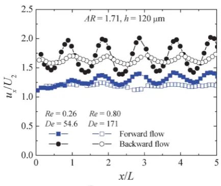
For higher flow rates, the flow becomes unsteady in both directions (scenario ii). In order to establish the overall evolution of the flow field and compare low and highDedata, in Fig. 7 we show the average axial velocity profiles obtained for the two scenarios and forh= 120mm. For unsteady flow conditions, the profiles were obtained using an average of 1000 image pairs. For the lowerDecases (scenario i), the difference in the amplitude of oscillation between the velocity profiles for both flow directions is notorious, in accordance with the results shown in Fig. 6.

For the backward direction, in which the flow remains steady, the velocity gradient at the centreline is higher than for the forward direction. Since, in the latter, we are averaging pairs of images acquired over a long period of time, in which the flow

behaviour was varying due to an elastic instability, the velocity fluctuations are smoothed out. At the higher De (cf. Fig. 7), when the flow is unsteady in both forward and backward directions, the amplitude of the average dimensionless velocity profile is lower than for lower elasticity flows especially for the backward flow direction. The differences between oscillating time-average forward and backward profiles are still noticeable, but smaller than at lowerDe. For the forward flow direction, a more plug-like velocity profile is observed for bothDe.

5.3. Wall effect on the diodicity

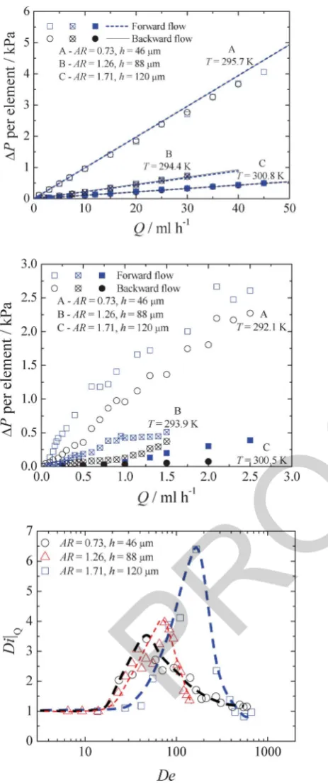
Fig. 8(a) shows the pressure drop per element of the rectifier measured experimentally as well as the corresponding numerical predictions for the Newtonian fluid flow through the hyperbolic rectifiers with different depths. Fig. 8(b) shows the pressure drop measured experimentally for the viscoelastic fluid. For both cases, the results obtained for the two flow directions are presented and are used to determine the variation of the diodicity of each microfluidic rectifier withDe.

As expected, for the same flow rate, the pressure drop observed in the microchannel with a smaller depth is significantly higher than that found for the deeper microchannel. For the Newtonian fluid, the pressure drop increases linearly with the flow rate, a consequence of the negligible inertial effects (in all casesr2¢0.991, whereris the sample correlation coefficient) . Furthermore, in agreement with the findings of Sousaet al.,27 negligible rectification effects are observed experimentally, i.e. for the same value of the flow rate, the corresponding forward and backward flow pressure drops are very similar, within experimental uncertainty. A good agreement between experi-mental and numerical results is observed. At the highest flow rates for the rectifier with h = 46 mm, small deviations are observed between the experimental data and the numerical predictions, but this is primarily due to the progressive defor-mation of the cross section area of the microchannels due to the high pressure differences required to obtain the higher flow rates (above 1.5 bar) and the corresponding deformation of the PDMS

Fig. 7 Dimensionless axial velocity profiles along the centreline of the hyperbolic rectifiers withh= 120mm for the viscoelastic fluid flow. At the lowerDe, the flow is unsteady in the forward flow direction and steady in the backward flow direction. At the higherDecases, the flow is unsteady in both flow directions.

Fig. 6 Time-average and instantaneous dimensionless axial velocity profiles along the centreline of the hyperbolic rectifier A (h= 46mm) for Re= 0.13 andDe= 32.9 (scenario i).

1

5

10

15

20

25

30

35

40

45

50

55

59

1

5

10

15

20

25

30

35

40

45

50

55

59

P

R

O

O

microchannels,38_{leading to a progressively smaller experimental}

flow resistance as the flow rate increases.

For the non-Newtonian fluid flow, despite the considerably lower flow resistance measured in the deeper channel, in qualitative

terms the overall behaviour is independent of the channel depth. At low flow rates, the pressure drop increases linearly with the flow rate, indicating a quasi-Newtonian flow behaviour. Increasing the flow rate (or De) beyond a critical value, the flow resistance becomes considerably different for the two flow directions, which is directly related with the onset of an elastic instability in the forward flow direction.24,27Above the critical flow rate, the flow resistance in the forward direction increases initially abruptly and then moderately as the flow rate increases. On the other hand, in the backward flow direction, the more pronounced increase of the flow resistance with the flow rate occurs only at significantly higher flow rates, since elastic instabilities in the backward flow direction also appear at higher flow rates. Hence, it is possible to infer, once again, that the changes in flow dynamics triggered by the onset of elastic instabilities lead to a markedly different flow resistance behaviour for both flow directions.

To better analyse the effect of the channel depth on the diodicity of the rectifier, in Fig. 8(c) we plot the diodicity, defined in terms of the pressure drop ratio for a constant flow rate, as a function ofDefor the three channel depths analysed.

The flow conditions corresponding to the maximum diodicity depend significantly on the aspect ratio of the channel as shown in Table 2.

As AR increases the Deborah number at which the peak diodicity was obtained also increases from about De = 45 for geometry A to De = 75 for geometry B and De = 165 for microchannel C. For microchannel A, having the lowest aspect ratio (AR= 0.73;h= 46mm), the maximum diodicity is about 3.5. For the intermediate microchannel B (AR= 1.26;h= 88mm) the maximum diodicity is about 4, while for the channel with the largest aspect ratio (AR = 1.71; h = 120 mm) the maximum diodicity is about 6.4. These values of diodicity are well above those previously achieved by other researchers.24,26

Thus, higher aspect ratios lead to higher rectification effects, suggesting that deeper geometries, where wall effects (or shear effects) are less pronounced and extensional flow is enhanced, may be preferred in order to devise efficient microfluidic diodes. It would be desirable to further increase the depth of the microfluidic diode, to investigate if higher diodicity would be achieved. However, using PDMS only moderate aspect ratio geometries can be replicated and other fabrication techniques need to be used to allow for precise fabrication of deeper microchannels. In any case, the map of diodicity displayed in Fig. 8(c), is valuable to determine the best rectifier for a wide range of flow rates, or at least of the best compromise between rectification effect and range of operation.

6. Conclusions

The flow of a Newtonian fluid (de-ionized water) and a non-Newtonian fluid with viscoelastic behaviour was investigated in

Fig. 8 Variation of the pressure drop per element of the rectifier, as a function of the flow rate and channel depth: (a) Newtonian fluid (symbols: experimental data; lines: numerical predictions), (b) viscoelas-tic fluid. (c) Diodicity as a function of Deborah number for the hyperbolic shaped rectifier with different depths. The dashed lines shown are a guide to the eye.

Table 2 Values of the Deborah number corresponding to the maximum diodicity for the three microchannels with different aspect ratios

AR De MaximumDi|Q

0.73 45 3.4

1.26 75 4.0

1.71 165 6.4

1

5

10

15

20

25

30

35

40

45

50

55

59

1

5

10

15

20

25

30

35

40

45

50

55

59

P

R

O

O

microfluidic rectifiers with hyperbolic shape to assess the effect of channel depth (aspect ratio) upon their diodicity. The Newtonian fluid flow was also simulated numerically and a good agreement with the experimental results was found. The fluid flow behaviour is qualitatively similar in the microgeome-tries with different depths. For the Newtonian fluid, the axial velocity at the centreline shows a periodic pattern due to geometric effects. At low inertial flow conditions, the velocity profile in the forward flow direction resembles that in the backward flow direction, while increasing the flow inertia leads to the appearance of a spatial offset between both velocity pro-files. For the viscoelastic fluid, different flow characteristics were found. At lowDe, the velocity profiles are Newtonian-like, but upon increasing the flow rate, the flow becomes unsteady and the axial velocity along the centreline of the microchannel varies in time, due to the onset of an elastic instability, which occurs at a lowerDein the forward flow direction than in the backward flow direction.

The measured pressure drop through the hyperbolic rectifiers shows a similar pattern for allAR. For the Newtonian fluid, the experimental results do not reveal noticeable rectification effects. In contrast, for the viscoelastic fluid, an anisotropic flow resistance is observed independently on the aspect ratio of the microchannel, but at different flow rate ranges. In terms of diodicity, the microfluidic rectifier with the highest aspect ratio presented a maximum diodicity of about 6.4, which is clearly in excess any other work reported in the literature The results suggest that, to some extent, reduction of shear and enhance-ment of the extensional component of the flow field (achieved by decreasing the effect of bounding walls) leads to higher diodicity.

Acknowledgements

The authors acknowledge the financial support provided by Fundac¸a˜o para a Cieˆncia e a Tecnologia (FCT) and FEDER through projects PTDC/EQU-FTT/71800/2006, REEQ/262/ EME/2005 and REEQ/928/EME/2005. P. C. Sousa would also like to thank FCT for financial support through scholarships SFRH/BD/28846/2006 and SFRH/BPD/75258/2010.

References

1 G. M. Whitesides,Nature, 2006,442, 368–373.

2 R. Go´mez-Sjo¨berg, A. A. Leyrat, D. M. Pirone, C. S. Chen and S. R. Quake,Anal. Chem., 2007,79, 8557–8563.

3 J. O. Tegenfeldt, C. Prinz, H. Cao, R. L. Huang, R. H. Austin, S. Y. Chou, E. C. Cox and J. C. Sturm,Anal. Bioanal. Chem., 2004,378, 1678–1692.

4 E. Verpoorte,Electrophoresis, 2002,23, 677–712.

5 J. deMello,Nature, 2006,442, 394–402.

6 H. A. Stone and S. Kim,AIChE J., 2001,47, 1250–1254. 7 K. L. Helton and P. Yager,Lab Chip, 2007,7, 1581–1588. 8 F. J. Tovar-Lopez, G. Rosengarten, E. Westein, K. Khoshmanesh,

S. P. Jackson, A. Mitchell and W. S. Nesbitt,Lab Chip, 2010, 10, 291–302.

9 S. Mall-Gleissle, W. Gleissle, G. H. McKinley and H. Buggisch, Rheol. Acta, 2002,41, 61–76.

10 M. S. N. Oliveira and G. H. McKinley,Phys Fluids (Letters), 2005, 17, 071704.

11 S. J. Muller, R. G. Larson and E. S. G. Shaqfeh,Rheol. Acta, 1989, 28, 499–503.

12 R. G. Larson, E. S. G. Shaqfeh and S. J. Muller,J. Fluid Mech., 1990, 218, 573–600.

13 P. Pakdel and G. H. McKinley,Phys. Rev. Lett., 1996,77, 2459. 14 P. E. Arratia, C. C. Thomas, J. Diorio and J. P. Gollub,Phys. Rev.

Lett., 2006,96, 144502.

15 R. J. Poole, M. A. Alves and P. J. Oliveira,Phys. Rev. Lett., 2007,99, 164503.

16 J. A. Pathak and S. D. Hudson, Macromolecules, 2006, 39, 8782–8792.

17 J. Soulages, M. S. N. Oliveira, P. C. Sousa, M. A. Alves and G. H. McKinley,J. Non-Newtonian Fluid Mech., 2009,163, 9–24. 18 M. S. N. Oliveira, F. T. Pinho, R. J. Poole, P. J. Oliveira and M. A.

Alves,J. Non-Newtonian Fluid Mech., 2009,160, 31–39.

19 H. Y. Gan, Y. C. Lam and N.-T. Nguyen,Appl. Phys. Lett., 2006,88, 224103.

20 A. Groisman and V. Steinberg,Nature, 2000,405, 53–55. 21 A. Groisman and V. Steinberg,Nature, 2001,410, 905–908. 22 A. Groisman and V. Steinberg,New J. Phys., 2004,6, 29–48. 23 A. Groisman, M. Enzelberger and S. R. Quake,Science, 2003,300,

955–958.

24 A. Groisman and S. R. Quake,Phys. Rev. Lett., 2004,92, 095401. 25 M. Navabi,Microfluid. Nanofluid., 2009,7, 599–619.

26 N.-T. Nguyen, Y.-C. Lam, S. S. Ho and C. L.-N. Low, Biomicrofluidics, 2008,2, 034101.

27 P. C. Sousa, F. T. Pinho, M. S. N. Oliveira and M. A. Alves,J. Non-Newtonian Fluid Mech., 2010,165, 652–671.

28 M. S. N. Oliveira, M. A. Alves, F. T. Pinho and G. H. McKinley, Exp. Fluids, 2007,43, 437–451.

29 Y. Xia and G. M. Whitesides,Angew. Chem., Int. Ed., 1998, 37, 550–575.

30 D. Meinhart, S. T. Wereley and M. H. B. Gray,Meas. Sci. Technol., 2000,11, 809–814.

31 J. Dealy and D. Plazek,Rheology Bulletin, 2009,78, 16–31. 32 N. Phan-Thien and R. I. Tanner, J. Non-Newtonian Fluid Mech.,

1977,2, 353–365.

33 P. J. Oliveira, F. T. Pinho and G. A. Pinto,J. Non-Newtonian Fluid Mech., 1998,79, 1–43.

34 M. A. Alves, P. J. Oliveira and F. T. Pinho,Int. J. Numer. Methods Fluids, 2003,41, 47–75.

35 R. B. Bird, R. C. Armstrong, O. Hassager,Dynamics of polymeric liquids.Volume 1: Fluid Dynamics, John Wiley & Sons, 1987. 36 S. T. Wereley and C. D. Meinhart,Micron-resolution particle image

velocimetry in micro- and nano-scale diagnostic techniques, Springer-Verlag, 2005.

37 M. A. Alves and R. J. Poole,J. Non-Newtonian Fluid Mech., 2007, 144, 140–148.

38 S. Hardy, K. Uechi, J. Zhen and H. P. Kavehpour,Lab Chip, 2009,9, 935–938.

1

5

10

15

20

25

30

35

40

45

50

55

59

1

5

10

15

20

25

30

35

40

45

50

55

59

P

R

O

O