Pressure-dependent network
water quality modelling
j1 Alemtsehay G. SeyoumMSc
PhD Student, Department of Civil Engineering, University of Strathclyde, Glasgow, UK
j2 Tiku T. TanyimbohPhD
Senior Lecturer, Department of Civil Engineering, University of Strathclyde, Glasgow, UK
j1 j2
Water quality models are increasingly being routinely used to help ascertain the quality of water in drinking water distribution systems for design and operational management purposes. Conventional water quality models are demand driven and consequently do not incorporate the effects of any deficiency in pressure on the water quality throughout the distribution network. This paper assesses a new integrated pressure-dependent hydraulic and water quality model. The model is an extension of the well-known Epanet 2 model that has an embedded logistic pressure-dependent nodal flow function. Hydraulic and water quality analyses based on two water supply zones in the UK were conducted for a range of simulated operating conditions including normal and subnormal pressure and pipe closures. It is shown that operating conditions with subnormal pressures, if severe and protracted, can lead to spatial and temporal distributions of the water age and concentrations of chlorine and disinfection by-products that are significantly different from operating conditions in which the pressure is satisfactory. The results presented may be indicative of modelling errors that may not have been recognised explicitly hitherto.
Notation
C reactant concentration in bulk flow Ccl chlorine concentration
CL ultimate trihalomethane (THM) concentration Cthm THM concentration
Hni head at nodei
kb reaction rate constant in bulk flow kf mass transfer coefficient
kw wall reaction rate constant Qni flow rate at nodei Qnreqi demand at nodei r(C) rate of reaction rh hydraulic radius of pipe
t time
u mean flow velocity x distance along pipe
Æ, parameters in the pressure-dependent demand function
1. Introduction
Water utilities routinely use water quality models to assess the quality of the water in their water distribution networks (WDNs). Water quality models can be used to investigate points in WDNs with long detention times, low disinfection residuals and exces-sive concentrations of disinfection by-products (DBPs). The models can also facilitate decision making for water quality
management. This includes the selection of sampling locations and sampling frequency, optimisation of the operation and the locations of booster disinfection stations. Water quality models have also been used to aid monitoring to help address concerns about possible deliberate contamination of water systems by terrorists (Skadsenet al., 2008).
WDNs are designed and operated to provide water that is wholesome to consumers at an adequate pressure. However, a major challenge in the operation of WDNs today arises from pressure-deficient conditions caused by events such as pipe breaks, pump failures or large increases in demand (e.g. for fire fighting purposes). These situations affect not only the hydraulic performance but also the quality of the water. Several studies have been conducted to evaluate the performance of WDNs under pressure-deficient conditions. These studies have focused on hydraulic analysis and addressed issues such as hydraulic relia-bility and design optimisation (Germanopoulos et al., 1986; Giustolisi et al., 2008; Tanyimboh and Kalungi, 2009) without considering water quality.
This may lead to bacterial regrowth (Clark and Haught, 2005) and, ultimately, water-borne diseases. Previous studies (Ghebre-michaelet al., 2008; Rodriguezet al., 2004) have also indicated that long detention times are a significant contributing factor in the formation of DBPs. DBPs are formed when the disinfectant reacts with organic and inorganic substances in water. They can cause reproductive and developmental problems in humans and are thought to be carcinogenic (Nieuwenhuijsen, 2005; Richard-sonet al., 2002). Many DBPs have toxic properties and can be mutagenic and genotoxic (Hebertet al., 2010). Therefore, given the self-evident deleterious effects of subnormal pressure on water quality, urgent action is required to integrate the hitherto separate water quality and pressure-dependent models.
Hydraulic and water quality analysis of WDNs can be performed under time-varying conditions by employing extended period simulation (EPS) models. The models include important time-varying features such as water levels in tanks, nodal demands and the scheduling of pumps. Conventional EPS models are demand driven and thus assume that all demands are fully satisfied even if a network is in a pressure-deficient condition. Consequently, EPS models based on demand-driven analysis (DDA) cannot simulate the performance of a pressure-deficient network realistically. Epanet 2 and Epanet-MSX are DDA-based EPS models whose use is widespread throughout the world. Epanet 2 (Rossman, 2000) is public domain software that can model non-reactive tracer materials, chlorine decay, DBPs growth and water age. Also in the public domain, Epanet-MSX (Shanget al., 2008) is an extension of Epanet 2 that can simulate multiple chemical species concurrently. Additional Epanet-MSX functionality in-cludes chloramine decomposition and bacterial regrowth.
In this paper, a new pressure-dependent analysis (PDA) model (Siew and Tanyimboh, 2012a) is discussed with particular refer-ence to water quality. This model, Epanet-PDX, is an extension of Epanet 2, which has an integrated pressure-dependent logistic demand function (Tanyimboh and Templeman, 2010). It has full Epanet 2 modelling functionality and can perform hydraulic, water quality and EPS analyses under both normal and pressure-deficient conditions in a seamless way. To assess the model, hydraulic and water quality analyses were conducted on two WDN ‘hydraulic demand zones’ in the UK based on demands the water utility provided for the purposes of hydraulic design optimisation. The properties considered are temporal and spatial variations in water age, chlorine and trihalomethane (THM) concentrations under various hydraulic conditions. Epanet 2 and Epanet-MSX results (for operating conditions with sufficient pressure) are also included for comparison and verification purposes. Given that Epanet 2 and Epanet-MSX are DDA models, they are unsuitable for pressure-dependent water quality investiga-tions. They are, however, included in this study to verify that Epanet-PDX water quality results for operating conditions with sufficient pressureare accurate.
Pressure-dependent demand functions are used in
pressure-dependent WDN models to achieve realistic estimates for operat-ing conditions with insufficient pressure and these functions require calibration for each demand node. When there is insufficient pressure, the flow delivered will be less than the demand. It has been shown that if the PDA predictions are accurate, then the PDA predictions of the nodal flows if used as demands in a DDA model will result in identical pipe flow rates, nodal flows and nodal heads in the DDA model (Ackley et al., 2001).
The aim of this paper is to demonstrate that, given identical hydraulic conditions of flow and pressure, Epanet-PDX yields essentially the same results for water quality as Epanet 2 and Epanet-MSX. Furthermore, by establishing that Epanet-PDX provides accurate hydraulic analyses for PDA and DDA subject to the pressure-dependent demand function imposed, it is demon-strated that Epanet-PDX can carry out both normal and pressure-deficient water quality modelling. In other words, given a set of demands for which the actual WDN pressure is insufficient, PDA identifies the feasible set of demands for which the available pressure would be sufficient that is ‘closest’ to the specified demands. Accordingly, these reduced demands can be modelled entirely satisfactorily using DDA (as stated above). It is thus sufficient here to show that Epanet-PDX yields accurate PDA predictions and that its water quality results are essentially the same as Epanet 2 and Epanet-MSX under normal operating conditions. A secondary aim is to demonstrate that, during pressure-deficient operating conditions, spatial and temporal variations in water quality can be very different from those in operating conditions with fully satisfactory pressure. The third aim of the paper is to illustrate the water quality modelling difficulties when low pipe flow velocities prevail due to excessive pressure reduction. As previous research (Tzatchkovet al., 2002) indicates, advection-driven models such as Epanet 2 may yield inconsistent water quality results if dispersion is significant due to low flow velocities.
2. Water quality modelling
The water quality model in Epanet 2 is dynamic and includes relevant fate processes such as transport (mainly advection) and various transformation processes (e.g. chlorine decay). In addition to pipe flow, some of the processes considered are mixing at pipe junctions, mixing in storage facilities, pipe wall reactions and a range of bulk flow reactions. Several modelling approaches for the chemical reactions are available, such as first- and second-order decay. The first-second-order reaction models are summarised briefly here. For chlorine decay
@Ccl
@t ¼ kbCcl
1:
@Cthm
@t ¼kb(CLCthm)
2:
where Cthm is THM concentration and CL is the ultimate THM concentration. For dissolved substances in water that react with materials at the pipe wall such as biofilm, the first-order model used is
@C
@t ¼
2kwkfC
rh(kwþkf) 3:
wherekwis the wall reaction rate constant,kf is the mass transfer coefficient (e.g. Rossman, 2000),rhis the hydraulic radius of the pipe andCis the reactant concentration in bulk flow.
The system of equations for conservation of mass that constitutes the water quality model can be set up by superposition of the relevant transport and transformation equations. For a pipe, for example, the equation that results is
@C
@t ¼ u
@C
@xþr(C)
4:
in whichuis the mean flow velocity,xis distance along the pipe and r(C) is the rate of reaction (e.g. Equations 1–3). Details of the complete water quality model based on advection and the computational solution procedure can be found in the literature (Rossman, 2000). An alternative approach that includes both advection and dispersion is described by Tzatchkovet al.(2002).
3. Pressure-dependent modelling
Pressure-dependent demand functions are often adopted to esti-mate actual flow at a demand node using the residual head at the node in question such that the demand is satisfied in full when the residual head is above a prescribed level and zero when the residual head is below the minimum acceptable level. Tanyimboh and Templeman (2010) proposed the following logistic pressure-dependent demand function that has no discontinuities (disconti-nuities in a demand function and its derivatives can cause convergence problems in the computational solution of the hydraulic equations)
Qni(Hni)¼Qnreqi
exp(ÆiþiHni)
1þexp(ÆiþiHni) 5:
where, for demand nodei, Qni is the flow rate,Hniis the head,
Qnreqi is the demand andÆi and i are parameters whose values
are determined by calibration using field data. Siew and Tanyim-boh (2012a) developed a pressure-dependent extension to Epanet 2 called Epanet-PDX by integrating this demand function into the global gradient algorithm (Todini and Pilati, 1988) that is the
hydraulic analysis model of Epanet 2. Epanet-PDX employs line minimisation to optimise iterative corrections of pipe flow rates and nodal heads. The EPS in Epanet-PDX consists of successive time intervals in which pressure-dependent steady-state analyses are performed that account for changes in nodal demands, water levels in tanks, the operation of pumps and the status of valves (Siew and Tanyimboh, 2010). Epanet-PDX is thought to have preserved the Epanet 2 modelling functionality (Rossman, 2000) in full. Thus, Epanet-PDX performs both hydraulic and water quality modelling under both normal and low-pressure conditions entirely seamlessly. The overriding objective here is to demon-strate this. Additional details on Epanet-PDX and recent literature reviews can be found in the papers by Siew and Tanyimboh (2012a, 2012b), Tanyimboh and Templeman (2010) and the references therein. Tanyimboh and Siew (2012) gave a recent comparison of WDN modelling practices with particular refer-ence to statutory and/or guideline requirements for flow and pressure at the point of delivery.
4. Demonstration examples
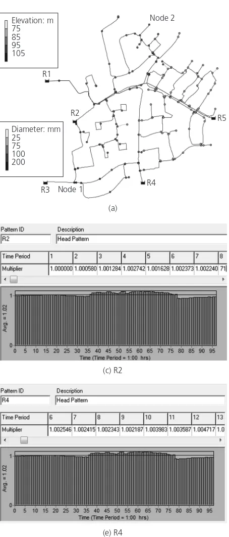
Extended period simulations were conducted on two ‘hydraulic demand zones’ (referred to hereafter as water supply zones) in the UK on an Intel Core 2 Duo personal computer (CPU¼3.2 GHz, RAM¼3.21 GB). For simplicity, the water supply zones are named here as networks 1 and 2 (Figures 1 and 2 respectively); 100% of all the analyses reported here for both networks are EPSs. Networks 1 and 2 obtain water entirely from neighbouring water supply zones through supply nodes (i.e. nodes R1–R5 in Figure 1 and nodes R1–R4 in Figure 2). The network and dynamic operational data used here for the hydraulic analyses were taken from calibrated Epanet models and a geographical information system (GIS) database. The Epanet models contain node data that include elevations and demands for individual nodes and the relevant demand categories.
j The demand categories in network 1 comprise domestic
demand, 10 h ‘commercial’ demand and unaccounted for water, for a duration of 96 h. Network 1 also has 29 different fire demands of 1 h each. These are applied at the 29 fire hydrants located at different positions in network 1.
j Network 2 has domestic demand, 10 h and 16 h ‘commercial’ demands and unaccounted for water. In all these demand types, demand multipliers are available every 15 min for 24 h total duration.
Also in the Epanet models are link data, including pipe lengths, diameters and roughness values; the Darcy–Weisbach pipe friction headloss formula (Rossman, 2000) was used for the hydraulic analyses. The information in the GIS database includes data on the pipes such as age, material, diameter, length, renewal and/or rehabilitation year, burst rate and other data of a geospatial nature.
typical or limiting values from the literature were assumed, as explained later. More fundamentally, this initial assessment, under artificially controlled operating conditions, is in fact a prerequi-site to the fieldwork and subsequent parameter calibration that will be required subsequently to address even more realistic and network-specific conditions that are inherently more complex and for which exact solutions will not be available. Collectively, the
subset of assumed modelling (i.e. reaction rate constants) and operational (i.e. chlorine concentration) values, when taken together with mandatory values stipulated in a selection of leading international standards for drinking water, are intended to represent the ‘most favourable’ scenario.
Accordingly, values ofkb¼0.5/day andkw¼0.1 m/day (Carrico Elevation: m
75 85 95 105
Diameter: mm 25
75 100 200
R3 Node 1 R4
R5 R2
R1
Node 2
(a) (b) R1
(c) R2 (d) R3
[image:4.595.43.270.127.658.2](e) R4 (f) R5
and Singer, 2009; Helbling and Van Briesen, 2009) were used. To achieve a detectable chlorine residual of 0.2 mg/l (WHO, 2011) at remote points in the system, the chlorine concentration at each supply node was assumed constant at 1 mg/l. Moreover, World Health Organization guidelines on drinking water quality (WHO,
2011) recommend a minimum residual chlorine concentration of 0.2 mg/l at the point of delivery; no minimum concentration value is stipulated in UK and EU drinking water standards. Also, the UK and EU standards do not specify a maximum concentration for chlorine; however, the values given in the WHO guidelines Elevation: m
85 95 100 105
Diameter: mm 50 100 200 300
R1 R3
R2
Node 3
R4
Node 4
(a) (b)
(c) (d)
[image:5.595.132.542.164.697.2](e) (f)
(WHO, 2011) and the US Safe Drinking Water Act, 1996 (US EPA, 1996) are 5 mg/l and 4 mg/l respectively (see e.g. Twortet al., 2000). It is recognised here that the taste and/or odour threshold is much lower; it may be noted that the typical concentration in most disinfected drinking water is 0.2–1.0 mg/l (WHO, 2011). A maximum total THM concentration of CL¼100ìg/l was adopted in Equation 2 based on EU and UK drinking water standards (EC, 1998; HMG, 2001, 2010); with a maximum concentration of 80ìg/l, the US EPA regulations are more stringent. Indeed, the EU and US standards advise that, where possible, a lower value should be aimed for without compromising disinfection. One of the drawbacks of the Epanet 2 THM model is that it requires modellers to specify the limiting THM concentration in advance. Sohnet al.(2004) suggested an alternative model for THM that avoids the need to pre-specify a limiting concentration (see e.g. Seyoum and Tanyimboh, 2013).
For both networks 1 and 2, the residual head for full demand satisfaction is 20 m; the (assumed) residual head below which nodal flow is zero is equal to the node elevation. To allow for the observed inconsistencies in the water quality results at the start of the simulations, the chosen EPS duration was 93 h for network 1 and 240 h for the much larger network 2; additional characterisa-tions of networks 1 and 2 are given later. The water quality results become stable after sufficient time has elapsed. The results reported here are for the last 30 h for network 1 and the last 24 h for network 2.
Both normal and low-pressure conditions were considered. The term ‘demand satisfaction ratio’ (DSR) here means the ratio of the flow available to the flow required (Ackleyet al., 2001). The DSR takes values from 0 to 1. Pressure-deficient conditions were created artificially by setting the water levels at the supply nodes to satisfy, in turn, only 90%, 75%, 50% and 30% of the total demand. A DSR of 30% is included to investigate water quality modelling in Epanet 2 under low-flow conditions with significant dispersion likely. The effects of closing individual pipes were also investigated.
In Section 5, for both network 1 and network 2, results are highlighted for two typical demand nodes that represent the nodes closest to the supply nodes (i.e. nodes 1 and 3 in Figures 1 and 2 respectively) and the remote points in the networks (i.e. nodes 2 and 4 in Figures 1 and 2 respectively). Results for the other demand nodes are not shown explicitly due to the limitations of space and for brevity. Additionally, variations in water age in the whole of network 1 are included for two different operating conditions – normal pressure (DSR¼100%) and a pressure-deficient condition (DSR¼75%). For all the EPSs for networks 1 and 2 1 hour and 15 minute hydraulic timesteps were used respectively, with water quality modelling concentration tolerance of 0.01 mg/l and water quality timestep of 5 min.
Figure 1 shows that network 1 consists of 251 pipes of various lengths, 228 demand nodes, 29 fire hydrants and five
variable-head supply nodes (R1 to R5); pipe diameters are 32–400 mm. Each variable-head supply node (Figure 1(b)–1(f)) has an average level of 155 m along with head level multipliers at 1 h intervals for a duration of 96 h. The range of variation in the head levels at each supply node is only [0.94, 1.10]. Hence, to simplify interpretation of the results, the supply nodes were modelled as constant-head nodes with water levels of 155 m each. Node 1 is close to supply node R3 while node 2 represents a remote point in the network. Considering various operating scenarios, 1838 EPSs of 93 h were carried out (see Table 1).
Network 2 (Figure 2) consists of 416 pipes of various lengths, 380 demand nodes and four supply nodes (R1 to R4). The pipe sizes range from 50 mm to 500 mm in diameter. R2, R3 and R4 are constant-head supply nodes with a water level of 133 m and R1 is a variable-head supply node. The head level multipliers for R1 are available at 15 min intervals in the range [0.94, 1.1], as shown in Figure 2(b). R1 was modelled here as a constant-head supply node using its average water level of 133 m (as explained previously for network 1). Nodes 3 and 4, respectively, were selected to represent nodes close to a supply node and remote points in the network. Network 2 has no hydrants or fire fighting flows. In total, 2534 EPSs of 240 h were performed (see Table 1). All results for network 2 appear to be entirely satisfactory. For this reason and due to limitations of space, only brief results are included for network 2 in the next section.
5. Results and discussion
5.1 Network 1: normal pressure
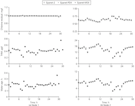
For initial verification purposes, water age, chlorine residual and THM were simulated using Epanet 2, MSX and Epanet-PDX under normal pressure (i.e. DSR¼100%), with the supply node heads fixed at 155 m. The three Epanet models provide essentially identical results, as shown in Figure 3, and the results are consistent with the demand fluctuations. An increase in residence time due to a reduction in demand is accompanied by a reduction in the concentration of chlorine and an increase in the water age and concentration of THM. The chlorine residual at node 1 is effectively constant due to its proximity to a supply node, where the concentration is kept constant. Taking water age as an example, the correlation coefficients between Epanet-PDX and Epanet 2 were R2¼1 for node 1 and R2¼1 for node 2. Similarly, the correlation between Epanet-PDX and Epanet-MSX wasR2¼1 for node 1 andR2¼0.999 for node 2. Epanet-MSX provides the water age, chlorine residual and THM concentration in a single simulation, while Epanet 2 and Epanet-PDX can simulate only one species at a time.
This further strengthens previous evidence (Siew and Tanyimboh, 2012a) that the results from the two models are essentially identical when there is sufficient pressure in the network. To complete the 93 h EPS, Epanet 2 and Epanet-PDX respectively required an average time of 0.7 s and 1.0 s for chlorine, 1.0 s and 1.4 s for THM and 0.6 s and 1.0 s for water age. Corresponding values for Epanet-MSX were 10.5 s for chlorine, 2 s for THM and 2 s for water age. The longer simulation time for chlorine is due to the simulation time associated with the wall reaction component of chlorine decay. To simulate chlorine, THM and water age concurrently, Epanet-MSX required an average time of 13 s (Table 2).
5.2 Network 1: pressure-deficient conditions
Simulations were carried out for several pressure-deficient condi-tions using Epanet-PDX. The constant heads at the supply nodes were reduced from 155 m to 105 m, 100 m, 95 m and 90 m to achieve network DSRs of 90%, 75%, 50% and 30% respectively. Figure 4 shows that Epanet-PDX provides different values of water age, chlorine residual and THM concentrations for the different low-pressure conditions and the greater the pressure deficiency the greater the water age and THM concentration and the smaller the chlorine residual concentration. This is consistent
with the fact that the greater the pressure deficiency the smaller the flow velocities in the network. The low flow velocities result in longer travel and residence times, which eventually lead to increased depletion of chlorine and formation of THM.
For node 1, it can be seen that there are large fluctuations in water age and chlorine and THM concentrations for DSR values of 50% and 30% for which the flow velocities are low in general. These fluctuations are consistent with previous results of the advection-driven Epanet 2 model, under conditions in which velocities are low (Tzatchkov et al., 2002). Tzatchkov et al. (2002) demonstrated that an advection–dispersion model reduced the fluctuations and consequently provided more realistic EPS results.
Figure 4 also shows that, from a water quality perspective, the effects of low pressure are more significant at remote points (node 2) than in an area close to a supply node (node 1). This is a direct consequence of the spatial distribution of water age. When DSR¼30%, the majority of nodes in network 1, including node 2, have very little or zero nodal flow. The results for node 2 when DSR¼30% would appear to reveal an anomaly. Zero- and low-flow nodes require special care and may indicate the need for
Number of EPSs
Network 1 Network 2
Epanet 2 Epanet-PDX Epanet-MSX Epanet 2 Epanet-PDX Epanet-MSX
Normal pressure
Water age 1 1 1 1 1 1
Chlorine 1 1 1 1 1 1
THM 1 1 1 1 1 1
Water age, chlorine and THM concurrently NAa NA 1 NA NA 1
Pressure-deficient conditionsb
Water age 4 4 NA 4 4 NA
Chlorine 4 4 NA 4 4 NA
THM 4 4 NA 4 4 NA
Water age, chlorine and THM concurrently NA NA 4 NA NA 4
Pipe closures
Water age 251 251 NA 416 416 NA
Chlorine 251 251 NA 416 416 NA
HM 251 251 NA 416 416 NA
Supply-node head variationsc(Figure 8(a)) 81 81 NA NA NA NA
PDA confirmation testsd 66 66 NA NA NA NA
Total 915 915 8 1263 1263 8
aNot applicable
bOne each for DSR¼90%, 75%, 50% and 30%
cIdentical demands and supply-node heads used for both Epanet 2 and Epanet-PDX dPDA low-pressure solutions confirmeda posterioriusing DDA
30 24
18 12
6 6 12 18 24 30
0·6 0·8 1·0 1·2
0
Chlorine r
esidual: mg/l
0·25 0·50 0·75 1·00
0
30 24
18 12
6 6 12 18 24 30
0 0
30 24
18 12
6 6 12 18 24 30
0 0
Epanet-2 Epanet-PDX Epanet-MSX
0 0·2 0·4 0·6 0·8
THM:
g/l
μ
0 6 12 18 24
0 0·1 0·2 0·3 0·4
W
ater age: h
Time: h (a) Node 1
0 4 8 12
[image:8.595.54.526.138.509.2]Time: h (b) Node 2
Figure 3.Water quality variations in network 1: (a) node 1; (b) node 2
Mean CPU time per EPS: s
Epanet 2
Epanet-PDX
Epanet-MSX
Network 1
Chlorine 0.70 1.00 10.50
THM 1.00 1.40 2.00
Water age 0.60 1.00 2.00
Chlorine, THM and water age concurrently NAa NA 13.00
Network 2
Chlorine 8.8 12.8 116.0
THM 12.6 16.5 23.0
Water age 9.1 12.5 17.0
Chlorine, THM and water age concurrently NA NA 146.0
aNot applicable
[image:8.595.38.352.568.749.2]more improvements in the underlying (Epanet 2) water quality model in the context of PDA. By contrast, Epanet 2 and Epanet-MSX provided the same results as the normal-pressure condition shown previously in Figure 3 because they lack PDA function-ality. This is illustrated in Figure 5, which shows Epanet 2 and Epanet-PDX predictions of water age throughout the network at 93 h for DSR values of 75% and 100%.
The effects of closing pipes one at a time were also investigated, with the heads at the supply nodes maintained at the normal level of 155 m. Figure 6 shows Epanet-PDX estimates of the
shortfall in the flow delivered (i.e. 1DSR). Whereas Figure 6 represents the entire network, the effects of low pressure can be greater in areas near closed pipes. Figure 7 depicts the water quality for Epanet 2 and Epanet-PDX for individual pipe closures. The results are comparable, apart for some slight differences in the chlorine residuals. Figure 6 shows that, overall, the pressure in the network is mostly satisfactory, with the DSR close or equal to 1. This explains the similarity between Epanet 2 and Epanet-PDX in Figure 7. In practice, it may not be possible to isolate individual pipes. Where multiple pipes must be taken out of service, it can be expected that any
30 20
10 30
20 10
0·88 0·92 0·96 1·00
0
Chlorine r
esidual: mg/l
0 0·3 0·6 0·9
0
30 20
10 0
1 2 3
0
THM:
g/l
μ
30 20
10 0
30 25 20 15 10 5
0 40 80 120 160
0
Time: h (b) Node 2 30
20 10
0 0 0·5 1·0 1·5 2·0
W
ater age: h
Time: h (a) Node 1
100% 90% 75% 50% 30%
[image:9.595.70.545.133.580.2]0 30 60 90 120
discrepancies due to the DDA modelling errors (i.e. in Epanet 2 for example) would be greater.
The computational efficiency of Epanet-PDX was assessed also with reference to Epanet 2 for the abovementioned water quality simulations. Figure 8(a) shows the results for a range of constant-head levels at the supply nodes. The average CPU time was 1.048 s per 93 h EPS simulation for Epanet-PDX and 0.640 s for Epanet 2 based on water age. Figure 8(b) shows the results for pipe closures. The average CPU time per 93 h EPS simulation for water age was 1.037 s for Epanet-PDX and 0.641 s for Epanet 2. Contrary to the results of Siew and Tanyimboh (2012a), the
results here together with the CPU times for the normal operating conditions in Section 5.1 that are based on a real system are an indication that Epanet-PDX may be slower than Epanet 2. The convergence criteria used in Epanet-PDX were 0.001 ft (3.0483104m) for the maximum change in the nodal heads and 0.001 cfs (2.8323105m3/s) for the maximum change in pipe flows between successive iterations. It is worth reiterating, however, that Epanet-PDX provides realistic results for pressure-deficient conditions whereas Epanet 2 does not.
A confirmation test was carried out on the PDA results as described in Section 1 (Ackleyet al., 2001; Siew and Tanyimboh, Age: h
20 40 60 80
(a) Epanet 2 (DSR⫽75%) (b) Epanet-PDX (DSR⫽75%)
[image:10.595.42.549.129.594.2](c) Epanet 2 (DSR⫽100%) (d) Epanet-PDX (DSR⫽100%)
2012a; Tanyimboh and Templeman, 2010) based on 66 constant supply-node heads from 90 m to 155 m in equal steps of 1 m for all the supply nodes. Siew and Tanyimboh (2012a) have pre-viously tested the accuracy of Epanet-PDX. Therefore (unlike the test in Section 5.1 that included all hydraulic timesteps), only the results of the last hydraulic timestep in each of the EPSs were
included in the present test. The correlation coefficients obtained were R2¼0.999 996 (or more simply 1R2¼43106) for nodal heads andR2¼0.996 for pipe flow rates based on 15 048 demand-node heads (66 supply-node heads3228 demand nodes) and 16 566 for pipe flow rates (66 supply-node heads3251 pipes). This confirms the accuracy of the Epanet-PDX hydraulic analysis results for subnormal pressures. In Section 5.1, the accuracy of the Epanet-PDX water quality results was demon-strated. It was shown that the Epanet-PDX results are essentially the same as those produced by Epanet 2 and Epanet-MSX, for identical regimes of flow and pressure. Therefore, confirmation here of the accuracy of the PDA results of Epanet-PDX also confirms the accuracy of the Epanet-PDX water quality results for operating conditions with subnormal pressure.
5.3 Brief results for network 2
For chlorine, total THM concentration and water age, the agreement between Epanet 2, Epanet-MSX and Epanet-PDX was excellent for normal operating conditions with sufficient pressure. 250
200 150
100 50
0·96 0·97 0·98 0·99 1·00
0
Network DSR
[image:11.595.60.291.136.237.2]Closed pipe ID
Figure 6.Epanet-PDX: pipe closure effects on the flow supplied in network 1
Epanet-PDX Epanet-2
250 200 150 100
50 0 50 100 150 200 250
250 200
150 100
50 0 50 100 150 200 250
0
250 200
150 100
50 0 50 100 150 200 250
Closed pipe ID (b) Node 2 0·85
0·90 0·95 1·00
0
Chlorine r
esidual: mg/l
0·50 0·55 0·60 0·65 0·70
0 3 6 9
THM:
g/l
μ
10 12 14 16 18 20
0 1 2 3 4 5
0
Age: h
Closed pipe ID (a) Node 1
5 6 7 8 9
[image:11.595.76.539.382.759.2]155 135 115 95 Epanet-PDX Epanet-2 250 200 150 100 50 0 0·4 0·8 1·2 1·6 75
CPU time: s
Supply node head: m (a) 0 0·4 0·8 1·2 0
[image:12.595.62.528.138.257.2]Closed pipe ID (b)
Figure 8.CPU times for network 1 based on water age: (a) supply-node head; (b) pipe closure
The percentages refer to the percentages of the total demand satisfied under normal and pressure-deficient conditions. 0·85
0·90 0·95 1·00
0 240 480 720 960 1200 1440 Node 3 Chlorine r esidual: mg/l Time: minutes 100% 100% 100% 100% 100% 100% 90% 90% 90% 90% 90% 90% 75% 75% 75% 75% 75% 75% 50% 50% 50% 50% 50% 50% 30% 30% 30% 30% 30% 30% 0 0·2 0·4 0·6 0·8
0 240 480 720 960 1200 1440 Node 4 Chlorine r esidual: mg/l Time: minutes 0 2 4 6 8
0 240 480 720 960 1200 1440 Node 3 TMH: g/l μ Time: minutes 0 18 36 54 72 90
0 240 480 720 960 1200 1440 Node 4 TMH: g/l μ Time: minutes 0 1 2 3 4
0 240 480 720 960 1200 1440 Node 3
W
ater age: h
Time: minutes
0 15 30 45
0 240 480 720 960 1200 1440 Node 4
W
ater age: h
Time: minutes
(a) (b)
(c) (d)
(e) (f)
Figure 9.Water quality in network 2 under normal and
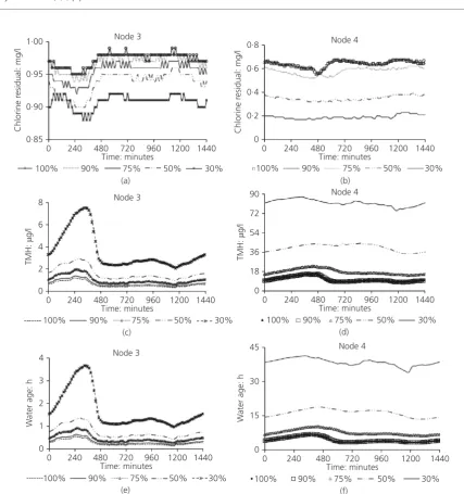
[image:12.595.66.494.285.741.2]As in network 1, the heads at the supply nodes were assumed constant. They were then reduced from 133 m to 112 m, 107 m, 102 m and 97 m, in turn, to obtain DSRs of 90%, 75%, 50% and 30% respectively. The daily demand and available flow patterns for nodes 3 and 4 can be seen in the supplementary data. Figure 9 provides a graphical summary of the water quality results for Epanet-PDX. In general the effects of pressure deficiency (from the water quality perspective) are greatest at the extremities of the network; the severity increases as the shortfall in pressure increases and temporal variations track the overall demand pattern (see, for example, Figures 2(c)–2(f). Unlike node 2 in network 1 for DSR¼30% that has almost zero flow, the water quality results at the remote node (node 4) follow the demand pattern. Also, the individual pipes were closed to simulate pipe failures. The results (not shown here) were very similar to the corresponding results for network 1 shown in Figure 7.
Table 2 compares the computational speeds of Epanet-PDX, Epanet 2 and Epanet-MSX for the water quality analyses under normal pressure conditions for the 240 h EPS. Based on these results, Epanet 2 is fastest and Epanet-MSX is slowest. Consider-ing that the EPS covers a period of 240 h (with a relatively small timestop of 15 minutes), the results suggest that Epanet-PDX may be fast enough for regular use.
6. Conclusions
Besides water age, this is the first paper to the authors’ know-ledge to address water quality modelling for low-pressure condi-tions in water distribution systems. This new approach is an extension of Epanet 2 that integrates pressure dependency with hydraulic and chemical analyses while preserving the modelling functionality of Epanet 2. Convergence difficulties or failures were not experienced with Epanet-PDX for the various cases considered in this study. Sample results based on two water supply zones in the UK are included; 4372 EPSs were performed in total using Epanet 2, Epanet-MSX and Epanet-PDX.
The results show that, if pressure is low, the conventional demand-driven modelling approach can provide misleading results that in turn can lead to inappropriate water quality policy decisions. An important corollary worth stating is that, under conditions of low pressure, poor demand-driven analysis estimates of the spatial distribution of the water age could mislead efforts intended to identify the source of accidental or intentional contamination. Finally, the results here have highlighted the need for more PDA-related work including the incorporation of dispersion in the water quality model and the collection of field data under conditions of low pressure, low flow rates and low velocities.
Acknowledgements
This project was funded in part by the UK Engineering and Physical Sciences Research Council (EPSRC grant reference EP/ G055564/1), the British Government (Overseas Research Students Awards Scheme) and the University of Strathclyde. This financial support is acknowledged with thanks. The authors also thank Dr
Lewis Rossman of the United States Environmental Protection Agency, who offered insights into the Epanet-PDX algorithm, computational performance and source code.
REFERENCES
Ackley JRL, Tanyimboh TT, Tahar B and Templeman AB(2001) Head driven analysis of water distribution systems. InWater Software Systems: Theory and Applications(Ulanicki B, Coulbeck B and Rance J (eds)). Research Studies Press, Taunton, UK, pp. 183–192.
Carrico B and Singer PC(2009) Impact of booster chlorination on chlorine decay and THM production: simulated analysis. Journal of Environmental Engineering135(10): 928–935. Clark RM and Haught RC(2005) Characterizing pipe wall
demand: implications for water quality modelling.Journal of Water Resources Planning and Management31(3): 208–217. EC (European Community)(1998) Council Directive 98/83/EC on
the quality of water intended for human consumption.Official Journal of the European CommunitiesL330.
Germanopoulos G, Jowitt PW and Lumbers JP(1986) Assessing the reliability of supply and level of service for water distribution system.Proceedings of the Institution of Civil Engineers Part 180(2): 413–428.
Ghebremichael K, Gebremeskel A, Trifunovic Net al.(2008) Modelling disinfection by-products: coupling hydraulic and chemical models.Water Science and Technology: Water Supply8(3): 289–295.
Giustolisi O, Kapelan Z and Savic D(2008) Extended period simulation analysis considering valve shutdowns.Journal of Water Resources Planning and Management134(6): 527–537. Hebert A, Forestier D, Lenes Det al.(2010) Innovative method
for prioritizing emerging disinfection by-products (DBPs) in drinking water on the basis of their potential impact on public health.Water Research44(10): 3147–3165.
Helbling DE and Van Briesen JM(2009) Modelling residual chlorine response to a microbial contamination event in drinking water distribution systems.Journal of Environmental Engineering135(10): 918–927.
HMG (Her Majesty’s Government)(2001) Water Supply (Water Quality) (Scotland) Regulations. Her Majesty’s Stationery Office, Edinburgh, UK, Scottish Statutory Instrument 2001 No. 207.
HMG(2010) Water Supply (Water Quality) Regulations. The Stationery Office, London, UK, Statutory Instrument 2010 No. 994 (W. 99).
Nieuwenhuijsen MJ(2005) Adverse reproductive health effects of exposure to chlorination disinfection by-products.Global NEST Journal7(1): 128–144.
Richardson SD, Simmons JE and Rice G(2002) Disinfection by-products: the next generation.Environmental Science and Technology36(9): 198A–205A.
Water Resources Division, National Risk Management Research Laboratory, US EPA, Cincinnati, OH, USA. Seyoum A and Tanyimboh TT(2013) Pressure-dependent
multiple-species water quality modelling of water distribution networks. Proceedings of 8th International Conference of European Water Resources Association, Porto, Portugal, pp. 553– 558.
Shang F, Uber JG and Rossman LA(2008) Modelling reaction and transport of multiple species in water distribution systems. Environmental Science and Technology42(3): 808–814. Siew C and Tanyimboh TT(2010) Pressure-dependent Epanet
extension: extended period simulation.Proceedings of 12th International Conference on Water Distribution Systems Analysis, Tucson, AZ, USA, CD-ROM.
Siew C and Tanyimboh TT(2012a) Pressure-dependent Epanet extension.Water Resources Management26(6): 1477–1498. Siew C and Tanyimboh TT(2012b) Penalty-free feasibility
boundary convergent multi-objective evolutionary algorithm for the optimization of water distribution systems.Water Resources Management26(15): 4485–4507, http://dx.doi.org/ 10.1007/s11269-012-0158-2, in press.
Skadsen J, Janke R, Grayman Wet al.(2008) Distribution system on-line monitoring for detecting contamination and water quality changes.Journal of American Water Works Association100(7): 81–94.
Sohn J, Amy G, Cho J, Lee Y and Yoon Y(2004) Disinfectant decay and disinfection by-products formation model development: chlorination and ozonation by-products.Water Research38(10): 2461–2478.
Tanyimboh TT and Kalungi P(2009) Multi-criteria assessment of optimal design, rehabilitation and upgrading schemes for water distribution networks.Civil Engineering and Environmental Systems26(2): 117–140.
Tanyimboh TT and Siew C(2012) Reference pressure for extended period simulation of pressure deficient water distribution systems. InASCE World Environmental and Water Resources Congress 2012: Crossing Boundaries (Loucks ED (ed.)). ASCE, Albuquerque, NM, USA, pp. 3257–3264.
Tanyimboh TT and Templeman AB(2010) Seamless pressure-deficient water distribution system model.Journal of Water Management163(8): 389–396.
Todini E and Pilati S(1988) A gradient algorithm for the analysis of pipe networks. InComputer Applications in Water Supply: System Analysis and Simulation, vol. 1 (Coulbeck B and Chun-Hou O (eds)). Research Studies Press, Taunton, UK, pp. 1–20.
Twort AC, Ratnayaka DD and Brandt MJ(2000)Water Supply. Arnold, London, UK.
Tzatchkov VG, Aldama AA and Arreguin FI(2002) Advection– dispersion–reaction modeling in water distribution networks. Journal of Water Resources Planning and Management 128(5): 334–342.
US EPA (United States Environmental Protection Agency)(1996) Safe Drinking Water Act, 1996. See http://water.epa.gov/ lawsregs/rulesregs/sdwa/index.cfm (accessed 18/07/2013). WHO (World Health Organization)(2011)Guidelines for
Drinking-water Quality. WHO, Geneva, Switzerland.
WHAT DO YOU THINK?
To discuss this paper, please email up to 500 words to the editor at [email protected]. Your contribution will be forwarded to the author(s) for a reply and, if considered appropriate by the editorial panel, will be published as a discussion in a future issue of the journal.