Infering and calibrating triadic closure in a dynamic network

Mantzaris, Alexander Vassilios and Higham, Desmond (2013) Infering

and calibrating triadic closure in a dynamic network. In: Temporal

networks. Springer, Berlin. ,

This version is available at

https://strathprints.strath.ac.uk/42880/

Strathprints is designed to allow users to access the research output of the University of Strathclyde. Unless otherwise explicitly stated on the manuscript, Copyright © and Moral Rights for the papers on this site are retained by the individual authors and/or other copyright owners. Please check the manuscript for details of any other licences that may have been applied. You may not engage in further distribution of the material for any profitmaking activities or any

commercial gain. You may freely distribute both the url (https://strathprints.strath.ac.uk/) and the

content of this paper for research or private study, educational, or not-for-profit purposes without prior permission or charge.

Any correspondence concerning this service should be sent to the Strathprints administrator: [email protected]

The Strathprints institutional repository (https://strathprints.strath.ac.uk) is a digital archive of University of Strathclyde research outputs. It has been developed to disseminate open access research outputs, expose data about those outputs, and enable the

Infering and Calibrating Triadic Closure in a

Dynamic Network

Alexander V. Mantzaris and Desmond J. Higham

AbstractIn the social sciences, the hypothesis of triadic closure contends that new links in a social contact network arise preferentially between those who currently share neighbours. Here, in a proof-of-principle study, we show how to calibrate a recently proposed evolving network model to time-dependent connectivity data. The probabilistic edge birth rate in the model contains a triadic closure term, so we are also able to assess statistically the evidence for this effect. The approach is shown to work on data generated synthetically from the model. We then apply this methodology to some real, large-scale data that records the build up of connections in a business-related social networking site, and find evidence for triadic closure.

1 Motivation

Many modern application areas give rise to patterns of connectivity that change over time [9]. Examples include mobile telecommunication, on-line trading, smart-metering, massive multiplayer online gaming and online social networking. Infor-mation such as ‘who called who’, ‘who tweeted who’, ‘who FaceTimed who’, and ‘people who bought his book also bought . . . ’ is naturally evolving over time and cannot be fully exploited through a static representation as a single time-average or snapshot. These emerging, data-rich disciplines generate large, highly-resolved network sequences that demand new models and computational tools.

This work focuses on the use of a mathematical model to describe the microscale, transient dynamics. The model, from [5], is mechanistic, incorporating the triadic closure effect that many social scientists believe to be a key driving force behind social interactions. We show how a likelihood approach can be used to calibrate the model, thereby allowing the triadic closure hypothesis to be tested statistically on real data.

Department of Mathematics and Statistics, University of Strathclyde, Glasgow, UK. e-mail: [email protected]

The manuscript is organised as follows. In Section 2 we introduce the triadic closure concept and discuss some relevant work in the area. In Section 3 we de-scribe the model from [5] and illustrate its use. Section 4 then explains how the likelihood—the probability of observing the microscale, edge by edge, data given a set of model parameters—can be computed and used to perform statistical infer-ence. To illustrate the idea, we generate synthetic data from the model and reverse engineer the model parameters. In Section 5 we then apply these ideas to a set of online social interaction data. Section 6 gives a summary and points to future work.

2 Background

The concept of triadic closure can be traced back to the work of the sociologist Georg Simmel in the early 1900s, and was popularized by the influential article [4]. It is a key motivation for the use of clustering coefficients [3, 15] to summarize network properties. The basic principle can be summarized as [2, 16]

Triadic Closure, part 1: If two unconnected people in a social network have a friend in common, then there is an increased likelihood that they will become friends themselves at some point in the future.

As discussed in [2, Chapter 3], there are at least three convincing reasons why triadic closure might feature in the evolution of a social interaction network. If B and C are not currently friends, but share a common friend, A, then a new link from B to C is more likely to arise than a link between an arbitrary pair, through

Opportunity: B and C both socialize with A and hence have more chance of meet-ing,

Trust: A can simultaneously vouch for both B and C,

Incentive: A may view the triadic friendship as less stressful or time-consuming to maintain than the separate pair of dyads, and hence encourage the B-C link.

Based on these points, we may also argue that each extra common friend shared by B and C will increase the chance of a future B-C link. Hence, we may slightly extend the triadic closure principle above:

Triadic Closure, part 2: The likelihood that two unconnected people in a social network will become friends themselves at some point in the future increases with the number of friends they share in common.

structures for positive and negative social interactions in a massive multiplayer on-line game and found “overrepresentation (underrepresentation) of complete triads in networks of positive ties, and vice versa for networks of negative ties.”

Networks in neuroscience have also been observed to have an overabundance of triangles, with respect to both anatomical and functional connectivity [1, 7, 13].

In this work we aim to go beyond the realm of simply recording the incidence of network triangles by combining ideas from applied mathematics and applied statis-tics. Given network data, we wish tocalibrate an appropriate mechanistic model of

network evolutionand simultaneouslyquantify the statistical evidence in favour of

triadic closure.

The closest previous work to ours is perhaps [12], where stochastic models incor-porating triadic closure were proposed and tested in a microscale/likelihood setting. To understand the class of models from [12], consider the nodeuin Figure 1 (which is based on Figure 6 from [12]). The triangulation stage adds a link to a node,w, that is two hops away fromu. This is done by first choosing one ofu’s neighbours, v, according to one of the five following rules

random: uniformly at random,

degree: proportional to some power of the degree of nodev,

common friends: proportional to the number of common friends shared by nodes uandv,

last time: proportional to some power of the time that has elapsed since vlast created an edge,

comlast: proportional to the product of (a) the number of common friends shared by nodesuandv, and (b) the time that has elapsed sincevlast created an edge, raised to some power.

Similarly, any of these five rules can be used to chose a neighbour,w, ofv. The new link is then inserted betweenuandwin order to create a triad. This gives a total 25 different models, which were tested in [12] on real data in a likelihood setting. The authors concluded that the random-random model (choose vuniformly from the neighbours ofuand then choosewuniformly from the neighbours ofv) gives a good compromise between accuracy and simplicity.

In this work, we consider a recent stochastic triadic closure model from [5], based on the general methodology of [6]. A key difference from the versions discussed above is that this model triangulates by directly choosing nodeswthat are two hops from u, with a bias that is proportional to the number of common neighbours— directly reflecting part 2 of the triadic closure principle. Advantages of this mod-elling approach are that:

• A single parameter,ε_{, is used to quantify the strength of the triadic closure effect.} The caseε_{=0 corresponds to no preference for triadic closure (edges appear} uniformly at some basal rate). Hence, we have a nested pair of models and can test whether there is statistically significant evidence for triadic closure in the data.

U

Y

W

V

Fig. 1: Depiction of the triangulation process, based on Figure 6 from [12]. A new edge is produced, as shown by the dashed line. This dashed edge creates a triad closure between nodes U, V, and W.

the same model parameters, and hence this macroscopic summary data can be used when a full likelihood computation at the microscale is not feasible. We exploit this feature in section 5.

3 The Triadic Closure Model

We suppose that a fixed set ofNnodes have a connectivity structure that may change at discrete, uniformly spaced, time pointst0<t1< . . . <tK. We letAk denote the adjacency matrix for the network at timetkand assume that the networks are un-weighted and undirected without self-loops, so eachAk∈RN×N hasai j=aji=1 if there is an edge from nodeito node jat timet_kand hasai j=aji=0 otherwise, with allaii=0.

The triadic closure model in [5] involves two matrix-valued functions of the cur-rent state,ω_{(Ak), and}α_{(Ak), giving theedge deathandedge birth probabilities,} respectively. The death probability takes the simple form

(ω_(Ak))

i j≡ω˜, for some ˜ω∈(0,1). (1)

The birth probability is defined as

(α_(Ak))

i j=δ+ε(A 2

for some constantsδ _andε_{. We impose 0<}ε_(N−2)<1−δ_{to ensure that the birth} probability lies between 0 and 1.

Given the timet_k network,A_k, if there is currently no edge from ito j, then the birth probability specifies the chance that the edge will emerge at time t_k+1. Similarly, ifiand jare connected inAk, the death probability specifies the chance that the edge will disappear at at timetk+1. Conditioned onAk, all such edge events are taken to be independent. More precisely, the model takes the form of a discrete time Markov chain over the state space of all binary, symmetric networks withN nodes, and givenA0we may simulate a path of the chain as follows

fork= 0,1, 2, ....,K−1 Computeα_(Ak)

for all disjoint pairsi6=j if(Ak)i j=0 then set

(Ak+1)i j=1 with prob.α(Ak)i j(birth)

(Ak+1)i j=0 with prob. 1−α(Ak)i j(no change) else we have(Ak)i j=1, so set

(A_k+1)i j=0 with prob. ˜ω_(death)

(A_k+1)i j=1 with prob. 1−ω˜ _{(no change)} end if

end for all pairs end fork

To understand the form of the birth probability (2), we note that the factor(A2_k)i j counts the number of neighbours shared by nodes i and j at time tk. Hence the overall birth probability is given by combining

• a basal level,δ_{, and}

• a triadic closure term that is proportional to the number of new triangles the edge would create. Hereε_{controls the strength of the triadic closure effect.}

A mean-field approximation for the evolution of a macroscopic quantity, the edge density

b

p_k:= 1

N(N−1)/2

∑∑

was proposed in [5] and found to match well with real simulations. This mean-field approximation takes the form

pk+1= (1−ω˜)pk+ (1−pk) δ+ε(N−2)p2k

. (4)

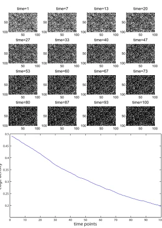
To illustrate the model, and also to provide some data for the inference compu-tations in the next section, we now show some network sequences generated by the model. In each case we used 100 nodes and 100 time points, and the initial network, A0, was a sample of a classical Erd¨os-R´enyi random graph with expected edge den-sity ofp; we denote this byA0=ER(p).

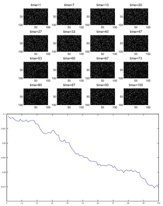
Data Set A:δ_{=0.0004, ˜}ω_=0.01,ε_{=0,A0=ER(0.5).}

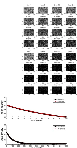
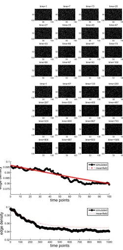
In this case there is no triadic closure–edges appear and disappear uniformly at random. The mean-field equation (4) collapses to a linear iteration with a single, stable steady state at p⋆=0.0385. Figure 2 shows the adjacency matrix at selected time points, along with the edge density as a function of time. The images of the adjacency matrix put a black square where the value is zero and a white square where the value is one. To show the relevance of the mean-field approximation, Figure 3 illustrates what happens when the path is followed for a longer period; we used 1000 time points. The mean-field approximation from (4) is superimposed over the edge density plots. Here the observed edge density at the final time point is 0.0356.

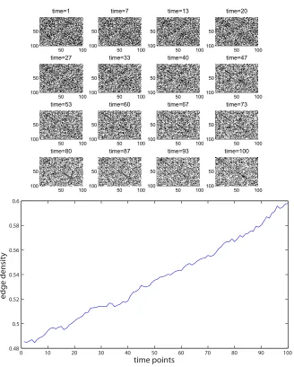
Data Set B:δ_{=0.0004, ˜}ω_=0.01,ε_{=0.0005,A0=ER(0.5).}

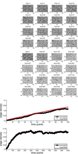
Here, the mean-field iteration has steady states 0.7215 (stable), 0.2291 (unstable) and 0.0494 (stable). Using A0=ER(0.5)starts the paths closest to the denser of the two stable macro-states. Figure 4 shows some network snapshots along with the edge density. A longer time interval is used in Figure 5 in order to confirm the relevance of thep⋆=0.7215 steady state.

Data Set C:δ_{=0.0004, ˜}ω_=0.01,ε_{=0.0005,A0=ER(0.1).}

Here, we use the same model parameters as in Data Set B, but start with a less dense initial network. Figure 6 shows network snapshots and edge density, and Figure 7 runs over a longer time period. In this case, the edge density is attracted to the other stable steady state atp⋆=0.0494.

4 Likelihood and Inference

The probabilistic nature of the model produces a natural likelihood function to feed into a calibration and inference framework. This section explains the details and tests out the idea on the data sets from Section 3.

Given network dataA0,A1, . . . ,Ak, that is, up to timetk, because the model sat-isfies the Markov property the likelikood of observing a networkAk+1at timetk+1 depends only onAkand is given by

L₍Ak+1|Ak) =

∏

(1−ω˜_)×

_∏

α_{(Ak)i j×}

_∏

Remain dead

(1−α_{) (Ak)i j×}

_∏

˜ ω_{i j.}

50 100 50

100

time=1

50 100 50

100

time=7

50 100 50

100

time=13

50 100 50

100

time=20

50 100 50

100

time=27

50 100 50

100

time=33

50 100 50

100

time=40

50 100 50

100

time=47

50 100 50

100

time=53

50 100 50

100

time=60

50 100 50

100

time=67

50 100 50

100

time=73

50 100 50

100

time=80

50 100 50

100

time=87

50 100 50

100

time=93

50 100 50

100

time=100

0 10 20 30 40 50 60 70 80 90 100

0.2 0.25 0.3 0.35 0.4 0.45 0.5

time points

edge density

50 100 50 100 time=1 50 100 50 100 time=7 50 100 50 100 time=13 50 100 50 100 time=20 50 100 50 100 time=27 50 100 50 100 time=33 50 100 50 100 time=40 50 100 50 100 time=47 50 100 50 100 time=53 50 100 50 100 time=60 50 100 50 100 time=67 50 100 50 100 time=73 50 100 50 100 time=80 50 100 50 100 time=87 50 100 50 100 time=93 50 100 50 100 time=100 50 100 50 100 time=1 50 100 50 100 time=67 50 100 50 100 time=133 50 100 50 100 time=200 50 100 50 100 time=267 50 100 50 100 time=333 50 100 50 100 time=400 50 100 50 100 time=467 50 100 50 100 time=533 50 100 50 100 time=600 50 100 50 100 time=667 50 100 50 100 time=733 50 100 50 100 time=800 50 100 50 100 time=867 50 100 50 100 time=933 50 100 50 100 time=1000

0 10 20 30 40 50 60 70 80 90 100

0.2 0.3 0.4 0.5 0.6 0.7 time points e d g e d e n si ty simulated meanfield

0 100 200 300 400 500 600 700 800 900 1000

0 0.2 0.4 0.6 0.8 time points e d g e d e n si ty simulated meanfield

50 100 50

100

time=1

50 100 50

100

time=7

50 100 50

100

time=13

50 100 50

100

time=20

50 100 50

100

time=27

50 100 50

100

time=33

50 100 50

100

time=40

50 100 50

100

time=47

50 100 50

100

time=53

50 100 50

100

time=60

50 100 50

100

time=67

50 100 50

100

time=73

50 100 50

100

time=80

50 100 50

100

time=87

50 100 50

100

time=93

50 100 50

100

time=100

0 10 20 30 40 50 60 70 80 90 100

0.48 0.5 0.52 0.54 0.56 0.58 0.6

time points

edge density

50 100 50 100 time=1 50 100 50 100 time=7 50 100 50 100 time=13 50 100 50 100 time=20 50 100 50 100 time=27 50 100 50 100 time=33 50 100 50 100 time=40 50 100 50 100 time=47 50 100 50 100 time=53 50 100 50 100 time=60 50 100 50 100 time=67 50 100 50 100 time=73 50 100 50 100 time=80 50 100 50 100 time=87 50 100 50 100 time=93 50 100 50 100 time=100 50 100 50 100 time=1 50 100 50 100 time=67 50 100 50 100 time=133 50 100 50 100 time=200 50 100 50 100 time=267 50 100 50 100 time=333 50 100 50 100 time=400 50 100 50 100 time=467 50 100 50 100 time=533 50 100 50 100 time=600 50 100 50 100 time=667 50 100 50 100 time=733 50 100 50 100 time=800 50 100 50 100 time=867 50 100 50 100 time=933 50 100 50 100 time=1000

0 10 20 30 40 50 60 70 80 90 100

0.5 0.55 0.6 0.65 0.7 time points e d g e d e n si ty simulated meanfield

0 100 200 300 400 500 600 700 800 900 1000

0.5 0.55 0.6 0.65 0.7 0.75 time points e d g e d e n si ty simulated meanfield

50 100 50

100

time=1

50 100 50

100

time=7

50 100 50

100

time=13

50 100 50

100

time=20

50 100 50

100

time=27

50 100 50

100

time=33

50 100 50

100

time=40

50 100 50

100

time=47

50 100 50

100

time=53

50 100 50

100

time=60

50 100 50

100

time=67

50 100 50

100

time=73

50 100 50

100

time=80

50 100 50

100

time=87

50 100 50

100

time=93

50 100 50

100

time=100

0 10 20 30 40 50 60 70 80 90 100

0.075 0.08 0.085 0.09 0.095 0.1

Fig. 6: Data set C. Upper: the adjacency matrix at selected time points. Lower: edge density as a function of time.

Now suppose that the model parameters and initial networkA0are fixed. Any observed network sequenceA1,A2, . . . ,AK then has likelihood

L₍A1|A0)×L(A2|A1)× · · · ×L(AK|AK−1). (5)

50 100 50 100 time=1 50 100 50 100 time=7 50 100 50 100 time=13 50 100 50 100 time=20 50 100 50 100 time=27 50 100 50 100 time=33 50 100 50 100 time=40 50 100 50 100 time=47 50 100 50 100 time=53 50 100 50 100 time=60 50 100 50 100 time=67 50 100 50 100 time=73 50 100 50 100 time=80 50 100 50 100 time=87 50 100 50 100 time=93 50 100 50 100 time=100 50 100 50 100 time=1 50 100 50 100 time=67 50 100 50 100 time=133 50 100 50 100 time=200 50 100 50 100 time=267 50 100 50 100 time=333 50 100 50 100 time=400 50 100 50 100 time=467 50 100 50 100 time=533 50 100 50 100 time=600 50 100 50 100 time=667 50 100 50 100 time=733 50 100 50 100 time=800 50 100 50 100 time=867 50 100 50 100 time=933 50 100 50 100 time=1000

0 10 20 30 40 50 60 70 80 90 100

0.075 0.08 0.085 0.09 0.095 0.1 time points e d g e d e n si ty simulated meanfield

0 100 200 300 400 500 600 700 800 900 1000

0.02 0.04 0.06 0.08 0.1 time points e d g e d e n si ty simulated meanfield

ranges. We focus here on theconstrained model, whereε_{is fixed at zero, so no triad} closure effect is present, and theunconstrained model, whereε_{is a model parameter.} The constrained model is therefore nested within the unconstrained model, which makes the application of the likelihood ratio test [18] suitable for model comparison. The likelihood ratio test value,D, is then used to compute a p-value for rejecting the null model, which is the constrained model. The valueDand the difference in de-grees of freedom in the unconstrained and constrained model are used as parameters for the chi-squared distribution. This allows us to compute a p-value for rejecting the null hypothesis. We take a threshold of 0.01.

The Akaike information criterion (AIC), [8], is also used here for model selec-tion. AIC is founded in information theory. The application of AIC reinforces the results of the likelihood ratio test.

Inference for Data Set A:

Here we performed a grid search of the likelihood overδ_{=0.0001 : 0.0001 : 0.0006} and ˜ω _{=0.0005 : 0.005 : 0.025 for the constrained model. For the unconstrained} model we also usedε_{=0.0000 : 0.0001 : 0.001.}

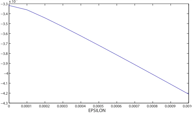
The search for the constrained model gaveα_{max =0.0004 and}ω_max=0.0105 with a log likelihood of−10182.0284. For the unconstrained model, we obtained α_max=0.0004,ω_{max=0.0105 and}ε_{max=0, with a log likelihood of−10182.0284.} Hence, the extra freedom offered byε_{was clearly not relevant for this data set. The} log likelihood ratio test therefore givesD=0, favouring the constrained model. The marginal forε_{is shown in Figure 8. We can see the decay away from the true value} of zero. AIC also prefers the model without triadic closure.

0 0.0001 0.0002 0.0003 0.0004 0.0005 0.0006 0.0007 0.0008 0.0009 0.0010

−4.3 −4.2 −4.1 −4 −3.9 −3.8 −3.7 −3.6 −3.5 −3.4 −3.3x 10

5

EPSILON

Inference for Data Set B:

Here we searched overα_{=0.0001 : 0.0001 : 0.0006 and}ω_{=0.0005 : 0.005 : 0.025} in the constrained model and alsoε_{=0.0000 : 0.0001 : 0.001 in the unconstrained} model. The likelihood for the constrained model is maximized atα_{max=0.0006 and} ω_{max=0.0105 with log likelihood of−38633.7891. For the unconstrained model,} α_max=0.0001,ω_{max=0.0105 and}ε_{max=0.0005 with log likelihood−31477.9615.}

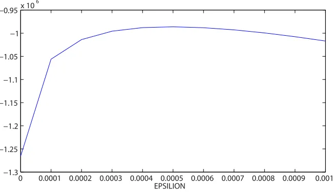
We note that the constrained model has a higher birth rate to compensate for the lack of triangulation. The log likelihood ratio test value isD=14311.6553, so the test result is 1, favouring the triad closure model. AIC chooses the model that has triad closure as well. The marginal ofε_{, shown in Figure 9, has a clear peak around the} value of 0.0005 that was used to generate the data.

0 0.0001 0.0002 0.0003 0.0004 0.0005 0.0006 0.0007 0.0008 0.0009 0.001 −1.3

−1.25 −1.2 −1.15 −1.1 −1.05 −1 −0.95x 10

6

EPSILION

Fig. 9: Marginal forε_{in Dataset B.}

Inference for Data Set C:

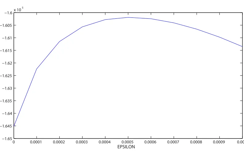
For the constrained model the grid search took place overα _{=0.0001 : 0.0001 :} 0.0006 andω _{=0.0005 : 0.005 : 0.025 and for the unconstrained model we also} usedε_{=0.0000 : 0.0001 : 0.001. The constrained model produced}α_max=0.0006 andω_{max=0.0105 with log likelihood of−5136.5503. For the unconstrained model} we haveα_max=0.0004,ω_{max=0.0105 and}ε_{max=0.0005 with log likelihood of} −5089.8203. As for Data set B, the constrained model has a higher birth rate to balance the lack of triangulation. The log likelihood ratio test value isD=93.4599, with a test result of 1, favouring the triad closure model. As well, AIC chooses the model with triad closure. The marginal ofε_{is shown in Figure 10, and, as in Data} set B, we see a peak around the value of 0.0005.

0 0.0001 0.0002 0.0003 0.0004 0.0005 0.0006 0.0007 0.0008 0.0009 0.001 −1.65

−1.645 −1.64 −1.635 −1.63 −1.625 −1.62 −1.615 −1.61 −1.605

−1.6x 10 5

EPSILON

Fig. 10: Marginal for epsilon for Data set C.

5 On-Line Social Network Data

We now apply this methodology to online social network data from [10] that relates to the Wealink (http://www.wealink.com/) social networking site for pro-fessionals in China. In this data set, new users (nodes) join the network over time, and a new link can be established between any pair of current users. The raw data consists of triples of the form(i,j,t), indicating that a link has been created between nodesiand jat time stampt. There are 26,817,840 time stamps, measured in sec-onds, and they range fromt=1 second to 72,711,888 seconds, which is just over 841 days. The largest node id is 223,482. For the purpose of calibration and model selection, we assume that all 223,482 nodes are present (i.e. available to form links) from the initial time point, and that all links are undirected. Hence we have sym-metric adjacency matrices of dimensionN=223,482. Edges do not disappear in this data set. Figure 11 shows how the edge density increases with time. The overall average rate of increase in Figure 11 is 0.0038 edges per second.

0 1e+007 2e+007 3e+007 4e+007 5e+007 6e+007 7e+007 8e+007 0

0.2 0.4 0.6 0.8 1 1.2 1.4 1.6

1.8x 10

−5 _{density every1000 seconds}

seconds

density

Fig. 11: Density of the Wealink online social network as a function of time in seconds.

Because of the large amount of data, we made a number of simplifications in order to reduce computational complexity to a feasible level. First, it is clear from Figure 11 that most activity takes place over a limited time period, and hence, for our experiments, we start with the network at time 3×107seconds and continue until time 4×107seconds. Then, rather than treating each event separately, we divide this period into 100 equally spaced time windows and construct an adjacency matrix for each. So each adjacency matrix records an element 1 in positions(i,j)and(j,i)if nodesiandjwere already linked, or formed a link in the relevant time window, and it records a zero otherwise.

Due to the excessive cost of evaluating the likelihood, we first used the mean-field approximation (4) to get a feel for an appropriate range of parameter values. Figure 12 shows the edge density increasing over the 100 discrete time points. The red circles show the corresponding mean-field solution when we fixε_{=0 and} opti-mize in a mean-square sense over the remaining parameter,δ_{; that is, givenp0, we} consider the iteration

pk+1=pk+ (1−pk)δ

nonzero; that is, we use

p_k+1=p_k+ (1−p_k) δ₊ε₍N−2)p2_k.

Here, we foundδ _=9.53×10−8_andε_=7.32×10−16_.

0 10 20 30 40 50 60 70 80 90 100 2

4 6 8 10 12x 10

−6

intervals

density

Fig. 12: Blue solid line: Edge density over the 100 discrete tme points used for the inference. Red circles: edge density from best mean-field fit withε_{fixed at zero and} δ _{as a free parameter. Black crosses: edge density from best mean-field fit with both} ε_andδ _{as free parameters.}

Since our available computing power only permitted a full likelihood based cal-ibration over one parameter, we then fixedδ _=9.95×10−8_{and infered the triadic} closure strength,ε_{, from the microscale data. Figure 13 shows the log likelihood as} a function ofε_{. The best}ε_{value gives a log likelihood of−1.58×10}8_{, whereas the} ε_{=0 model produces−1.97×10}8_{. We find thatD=7.81×10}7_{, and the triadic}

closure model is therefore chosen by the log likelihood ratio test. AIC also chooses the model with triadic closure.

6 Summary

−25 −20 −15 −10 −5 0 5 −1012

−1011 −1010 −109 −108

Exponent

Log Likelihood

Fig. 13: Log likelihood of the triadic closure model as a function of triad closure strength,ε_{. The basal edge birth is fixed at 9.95×10}−8_{. The x-axis shows the log} base 10 values used forε_{in the search for the largest loglikelihood.}

Although likelihood-based calibration and model comparison is conceptually straightforward for stochastic, Markov chain based, models of the type used here, the fundamental task is computationally challenging for large network sequences over long time periods. In this work, we were able to exploit a mean-field theory that describes the evolution of a macroscale quantity—the edge density—in terms of the model parameters.

There are many directions in which this type of work could be taken:

• other concepts from the social sciences that may determine network dynamics, such as homophily/heterophily, social distance and cultural drift [2, 11], could be quantified through mathematical models and then tested for and compared in real dynamic data sets,

• other types of interaction network, for example from telecommunication, online human behaviour and e-business, could be calibrated, compared and categorized, • more sophisticated, customized strategies for sampling the model parameter space could be developed; for example via Markov chain Monte Carlo tech-niques.

Acknowledgment

References

1. Bullmore, E., Sporns, O.: Complex brain networks: graph theoretical analysis of structural and functional systems. Nature Reviews Neuroscience10, 186–198 (2009)

2. Easley, D., Kleinberg, J.: Networks, Crowds, and Markets: Reasoning About a Highly Con-nected World. Cambridge University Press (2010)

3. Estrada, E.: The Structure of Complex Networks. Oxford University Press, Oxford (2011) 4. Granovetter, M.: The Strength of Weak Ties. The American Journal of Sociology78(6), 1360–

1380 (1973)

5. Grindrod, P., Higham, D.J.: Evolving graphs: Dynamical models, inverse problems and prop-agation. Proceedings of the Royal Society, Series A466, 753–770 (2010)

6. Grindrod, P., Higham, D.J.: Bistable evolving networks (To appear in Internet Mathematics) (2012)

7. He, Y., Chen, Z.J., Evans, A.C.: Small-world anatomical networks in the human brain revealed by cortical thickness from MRI. Cerebral Cortex17(10), 2407–2419 (2007)

8. Hirotugu, A.: A new look at the statistical model identification. IEEE Transactions on Auto-matic Control19(6) (1974)

9. Holme, P., Saram¨aki, J.: Temporal networks. Physics Reports519, 97–125 (2012)

10. Hu, H., Wang, X.: Evolution of a large online social network. Physics Letters A373(1213), 1105–1110 (2009)

11. Jackson, M.O.: Networks and economic behavior. The Annual Review of Economics1, 489– 513 (2009)

12. Leskovec, J., Backstrom, L., Kumar, R., Tomkins, A.: Microscopic evolution of social net-works. In: Y. Li, B. Liu, S. Sarawagi (eds.) KDD, pp. 462–470. ACM (2008)

13. Liu, Y., Liang, M., Zhou, Y., He, Y., Hao, Y., Song, M., Yu, C., Liu, H., Liu, Z., Jiang, T.: Disrupted small-world networks in schizophrenia. Brain131(4), 945–961 (2008)

14. Mislove, A., Koppula, H.S., Gummadi, K.P., Druschel, P., Bhattacharjee, B.: Growth of the Flickr Social Network. In: Proceedings of the 1st ACM SIGCOMM Workshop on Social Networks (WOSN’08). Seattle, WA (2008)

15. Newman, M.: Networks: An Introduction. Oxford University Press, New York (2010) 16. Rapoport, A.: Spread of information through a population with socio-structural bias. The

Bulletin Of Mathematical Biology15(4), 523–533 (1953)

17. Szell, M., Thurner, S.: Measuring social dynamics in a massive multiplayer online game. Social Networks39, 313–329 (2010). URL http://arxiv.org/abs/0911.1084