Multilevel Modelling with Spatial Effects

S

TRATHCLYDE

D

ISCUSSION

P

APERS IN

E

CONOMICS

D

EPARTMENT OF

E

CONOMICS

U

NIVERSITY OF

S

TRATHCLYDE

G

LASGOW

MULTILEVEL

MODELLING

WITH

SPATIAL

EFFECTS

B

Y

LUISA CORRADO AND BERNARD FINGLETON

Multilevel Modelling with Spatial Effects

This Version: February 2011

Abstract

In multilevel modelling, interest in modeling the nested structure of hierarchical data has been accompanied by increasing attention to di¤erent forms of spatial interactions across di¤erent levels of the hierarchy. Neglecting such interactions is likely to create problems of inference, which typically assumes independence. In this paper we review approaches to multilevel modelling with spatial e¤ects, and attempt to connect the two literatures, discussing the advantages and limitations of various approaches.

Key-Words: Multilevel Modelling, Spatial E¤ects, Fixed E¤ects, Random E¤ects, IGLS, FGS2SLS.

L. Corrado* & B. Fingleton**

* Marie Curie Fellow, Faculty of Economics, University of Cambridge,

UK and University of Rome II, Italy.

E-mail:[email protected]. Luisa Corrado acknowledges the support of the

Marie-Curie IE Fellowship 039326.

**Professor of Economics, Strathclyde University.

1

Introduction

Multilevel models are becoming increasingly popular across the range of the social sciences, as re-searchers come to appreciate that observed outcomes depend on variables organised in a nested hier-archy. 1 _{We see many applications of multilevel modelling in educational research where there exist} a number of well de…ned groups organized within a hierarchical structure, such as the teacher-pupil relationship, leading to the analysis of e¤ects on individual pupil behaviour coming from di¤erent hierarchical levels. For example, irrespective of personal attributes and other factors, being in the same classroom will tend to cause pupil performance to be more similar than it otherwise would be. This suggests that once the grouping has been established, even if its establishment is random, the group itself will tend to become di¤erentiated. This implies that the group and its members can both in‡uence and be in‡uenced by the composition of the group (Goldstein (1998)). In geograph-ical studies, we can often envisage a hierarchy of e¤ects from cities, regions containing cities, and countries containing regions. Failure to recognise these e¤ects emanating from di¤erent hierarchical levels can lead to incorrect inference. However while the standard approaches to multilevel analysis are well established, there is none the less much scope for the re…nement and development of this extremely useful methodology. In this paper we focus on interdependencies beyond those intra-class correlations that exist because individuals are taught in the same class room, or coexist within the same region. The innovation in this paper is that we take this wider perspective on interdependencies, drawing particularly on the burgeoning literature of spatial econometrics (Anselin (1988a)). This ac-commodates spatial dependence within cross-sectional regression models, and also within panel data analysis. In our review, we explore the connections between conventional multilevel models and the kinds of models proposed by spatial econometricians. Naturally, as economists, most of our examples and motivation are drawn from economics, and from economic geography, although we believe that the approaches we consider have much wider potential application.

In economics, considerable recent attention has been given to spatial economics and international trade, particularly with the advent of the ‘new economic geography’ (Fujita and Krugman (1999)). The increasingly spatial perspective means that very often we are faced with cross-sectional data indexed by location rather than time, or panel data in which each time layer comprises a data set of location-speci…c observations. In economic geography, with a hierarchy of local, regional and national e¤ects typically in‡uencing outcomes, the obvious starting point is multilevel modelling, in which individual level cross-sectional (spatial) data within the same local administrative area, for example, are subject to an e¤ect because of their common location. Perhaps local property taxes are di¤erent across local administrative units, and properties, which are the units of observation, have prices partly re‡ecting these local tax di¤erences. Additional spatial e¤ects may arise at di¤erent levels of a nested hierarchy; for instance we may wish also to control for the e¤ects of being located within the same region, perhaps because policy instruments having an e¤ect on property prices are applied at the regional level and are di¤erent from the e¤ects of local tax di¤erentiation.

The contribution of the spatial econometrics perspective is that it introduces the notion that the analysis of spatial e¤ects simply via the e¤ects of multilevel group membership (local, regional, national) may be inadequate as a means of totally capturing the true spatial dependencies in the data, and this can produce misleading outcomes. For example, real estate prices may be a¤ected

1

by individual level real estate attributes (size of plot etc.) and by hierarchical location e¤ects (local administrative area e¤ects, regional e¤ects etc.), but there could also be an interaction between neighbouring properties that depends on, say, distance, so that the intra-area correlation between individual properties is unequal, due to the di¤erent distances between properties within areas, and moreover, the correlation does not terminate abruptly at area boundaries, but spills over. This spilling over of externalities across space will lead to unmodelled e¤ects (the error), or indeed prices directly, being spatially autocorrelated. Modelling such externalities comes within the realm of spatial econometrics. By not properly modelling these spatial interdependencies, with positive dependence, the outcome could be that, since the actual information content is smaller than that implied by the actual sample size, using the data as though they were independent leads to standard errors that are biased downwards. Therefore alongside the nested structure of the hierarchical data increasing attention has been paid to di¤erent forms of interactions and externalities in the hierarchical system (Durlauf (2003), Manski (2000), Brock (2001), Akerlof (1997)). As another example, Bénabou (1993), Durlauf (1996), Fernandez and Rogerson (1997) consider the e¤ects of residential neighbourhood on education. Typically we will …nd that a child’s education is determined, at least in part, by factors such as school quality, but the characteristics of other pupils with whom the pupil interacts, captured possibly by a social network structure, will also be of relevance. The importance of such externalities has led researchers to de…ne di¤erent concepts of membership and neighborhood e¤ects relying on notions of distance in social space (Akerlof (1997), Anselin (2002)). Widespread use has been extended to health research where for example multilevel modelling with spatial dependence has been applied to examine the geographical distribution of diseases, since diseases often spread due to contagion via contact networks (see, Langford, Leyland, Rasbash, and Goldstein (1999)).

Recognition of the di¤erent form of interactions between variables which a¤ect each individual unit of the system and the groups they belong to has important empirical implications. In fact, regardless of spatial autocorrelation, the assumption of independence is usually incorrect when data are drawn from a population with a grouped structure since this adds a common element to otherwise independent errors, thereby inducing correlated within group errors. Moulton (1986) …nds that it is usually necessary to account for the grouping either in the error term or in the speci…cation of the regressors. Apart from within- group errors, it is also possible that errors between groups will be correlated. For example, if the groups are geographical regions then regions that are neighbours might display greater similarity than regions that are distant. Again, Moulton (1990) shows that even with a small level of correlation, the use of Ordinary Least Squares (OLS), will lead to standard errors with substantial downward bias and to spurious …ndings of statistical signi…cance.

One way of incorporating the group e¤ect in a multilevel framework is to evaluate the impact of higher level variables on the individual which measure one or more aspects of the composition of the group to which the individual belongs. Bryk and Raudenbush (1992) consider di¤erent ways of doing this, such as using a simple mean covariate over the higher level units as an explanatory variable. The mean covariate characterizes group e¤ects which are measurable and in this respect di¤ers from the use of dummy variables which capture the net e¤ect of several variables. Note that it is possible that having controlled for these measurable compositional e¤ects there are still unobservable spatial e¤ects.

non-diagonal covariance matrix. As with unconditional ANOVA this will provide the decomposition of the variance for the random e¤ect into an individual component and a group component. Under a spatial dependence process acting at the level of random group e¤ects, the random components are typically a¤ected by those of neighbouring groups. This assumption is usually a relaxation of the main hypothesis in hierarchical modelling, i.e. independence between groups. As we have seen, especially when the groups are geographical areas, this might often be unrealistic.

The paper is organized as follows. The following section presents a diagrammatic representation of the multilevel modelling approach. Section two describes how to model spatial e¤ects through the error term; it also describes di¤erent ways of de…ning spatial and multidimensional weighting matrices. Sections three illustrates how to estimate linear random intercept models. Sections four and …ve illustrate how to accommodate correlation between predictors and (group) spatial e¤ects using …xed or random e¤ects in multilevel models. Section six links multilevel to spatial models, illustrates how to identify the relevant parameters for the group random e¤ects and the endogenous spatial lag and connects multilevel modelling to recent developments in panel data analysis, highlighting where progress might be made in estimation methodology. Section seven concludes.

1.1 A Representation of a Multilevel Structure

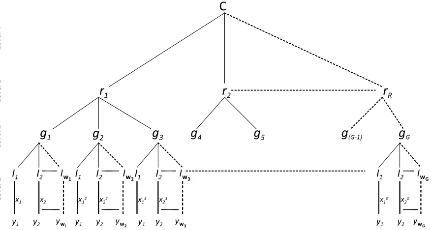
Figure 1 represents a diagrammatic representation of a multilevel hierarchy. Here with R denoting the top level,N the second level, andI the individual level. There is a variable number of individuals per second level group, and varying numbers of second level groups in each category at the top level of the hierarchy. In the context of spatial data we might consider a geographical grouping of individuals with the highest level being R regions (r) each of which nests a total of G smaller geographical sub-regions (g): These sub-regions may be either speci…c areas of residence or some other relevant geographical units. Located within each sub-region there are individuals(I) with a variable number of individuals per sub-region.

We associate with each individual a response Yi which is dependent upon a set of covariates Xi.

However, in assessing whether we might assign any causal relationships between one or more elements ofXiand the individual response Yi, it is necessary to consider the hierarchical structure of the data,

and in particular within- and between-group e¤ects.

non-independence while having no impact on point estimates, MLM provides us with estimates of the variance components at each level and these a¤ect point estimates directly. In turn, variances and covariances constitute valuable information on the contribution of non-observable factors at each level to the variation of the dependent variable (Aslam and Corrado (2007)).

2

Modelling spatial e¤ects through the error term

Below we introduce the basic multilevel model focussing on the two level case. We write this model as:

Yij = 0+Xij 1+Zj +"ij; (1)

whereYij denotes the response,Xij is a1 kvector of covariates,Zj is a(1 q )vector of group level

2 explanatory variables (invariant within groups) and"ij is the random disturbance;i,i= 1; : : : ; N

and j,j = 1; : : : ; G;denote, respectively, level 1 and level 2 units. We write the error term as:

"ij =eij+uj; (2)

where"ij denotes an additive error term composed of a random error termeij for theithunit belonging

to levelj and a random e¤ect uj for each level 2 unit. We make the following assumptions:

eijjXij N(0; e) Cov(eij; ei0j) = 0;8i6=i0

ujjXij N(0; u) Cov(uj; eij) = 0

(3)

We let 2_e ( 2_u) denote the variance of eij (uj) such that for cov(eij; uj) = 0, then 2" = 2e + 2u

represents the sum, respectively of the within- and between-group variances. Based upon the above, we may write the (equicorrelated) intra-class correlation as:

=

2

u

2

u+ 2e

: (4)

This correlation measures the proportion of the variance explained at the group level. In single-level models 2_u = 0 and 2_" = 2_e becomes the standard single level residual variance.

Following Anselin, Le Gallo, and Jayet (2007), who write from a spatial panel data perspective, there are four ways we might wish to model spatial e¤ects operating through the error term, namely i) direct representation, which originates from the geostatistical literature (Cressie (2003)); as noted by Anselin (2003), this requires exact speci…cation of a smooth decay with distance and a parameter space commensurate with a positive de…nite error variance-covariance matrix. Alternatively, as in Conley (1999), a looser de…nition of the distance decay may be implemented, leading to non-parametric estimation; ii) spatial error processes typi…ed by much work in spatial econometrics (Anselin (1988a)), based on a so-called W matrix de…ning indirectly the spatial structure of the non-zero elements of the error variance-covariance matrix. The W matrix comprises non-negative values representing the a priori assumption about interaction strength between location pairs de…ned by speci…c rows and columns of W, normally with zeros on the main diagonal. Typically but not necessarily W is normalized to sum to 1 across rows; iii) common factor models originating from the time series literature (Hsiao and Pesaran (2004), Pesaran (2007), and Kapetanios and Pesaran (2005)) and iv) spatial error components models (Kelejian and Robinson (1995), Anselin and Moreno (2003)) combining local (eij) and spillover(uj) error components. To accommodate these e¤ects we rewrite

"ij =eij +

X

j6=h

ujWjh; (5)

where W = _fWjhg allows us to specify the way neighbouring areas a¤ect uj: The matrix W is a

matrix of distances between the G entities as discussed below. The intra-class correlation is now given by:

=

2

u

P

j6=h 2uWjh2 + 2e

: (6)

One simple way to allow for these e¤ects is to set Wjh= 1(j^h)where1(:) is the indicator function

and j_^h denotes the contiguity of area j with area h: Trivially if W = I;where I is the identity matrix, then we have the standard random e¤ects model ignoring any between group e¤ect.

If uj are treated as …xed parameters then we need to assume that cov(eij; uj) = eu = 0, that

is transient individual-level random e¤ects are uncorrelated with, say, a level 2 variable such as the area of residence. If uj and eij are not independent the Generalised Least Squares (GLS) estimator

would be biased and inconsistent. If uj are permanent random e¤ects we also assume independence

between these and the covariates such that cov(Xij; uj) = ux = 0 (Blundell (1997)). Relaxing the

constraints ux6= 0 and eu6= 0 is discussed in sections …ve and six.

2.1 Spatial versus Multidimensional Weighting Matrices

In the following paragraphs we illustrate some of the traditional distance-based unidimensional sures adopted in spatial econometrics (Anselin (1988b)) and introduce other multidimensional mea-sures based on various notions of social or economic distance. Typically, isotropy is assumed, so that only distance between j and h is relevant, not the direction j toh. These may provide the basis for direct or indirect estimation of the error variance-covariance matrix, including the spillover in error components models.

Spatial externalities can sometimes re‡ect not only pure spatial interaction but other important substantive multiple phenomena at the economic, political, cultural and institutional level operating at the group (or area) level (Tienda (1991)). For example, in community psychology (O’Campo (2003)) often the de…nition of neighbourhood is based on respondents’perception of their own neighborhood as well as on economic and census data (Aronson and Brodsky (1999); Ross, Reynolds, and Geis (2000); Shumow, Vandell, and Posner (1998)). Analysis of social exclusion (Muntaner, Lynch, and Oates (1999); Ross, Reynolds, and Geis (2000)) and social segregation Goldstein and Noden (2003) often considers geographical position as one among several factors that weaken the links between individuals and the rest of society.

Crude measures of between group spatial ‘distance’ include simple notions of proximity and contiguity, concepts which have motivated the work of Cli¤ and Ord (1973) and Cli¤ and Ord (1981) and speci…cally the measure of spatial autocorrelation. Cli¤ and Ord (1973) combines distance and length of the common border thus :

Wjh = (djh)a jh b

(7)

wheredjh denotes the distance between locationsj andh and jh is the proportion of the boundary

of j shared withh whereas aand bare parameters.

Wjh= exp( djh) (8)

with controlling the strength of a distance-decay e¤ect. Dacey (1968) suggests that

Wjh =bjh j jh (9)

in which bjh is a binary contiguity factor, j is the share of unitj in the total area of all the spatial

units in the system, and _jh is the same boundary measure as used in (7).

The above measures apply mostly to physical features of geographical units. However, they are less useful when spatial units consist of points and when the spatial interaction is determined by purely economic variables which may have little to do with spatial con…guration of boundaries. Economic distance has been a feature of work by Conley (1999), Pinkse, Slade, and Brett (2002), Conley and Topa (2002), Conley and Ligon (2002) and Slade (2005). For example Conley and Ligon (2002) estimate the costs of moving factors of production. Physical capital transport costs are related to inter-country package delivery rates, and the cost of transporting embodied human capital is based on airfares between capital cities (the correlations with great circle distances are not perfect). In their analysis, for practical reasons, they con…ne their analysis to single distance metrics, but they prefer multiple distance measures. Taking the wider perspective of the industrial organization literature, distances may be in terms of trade openness space, regulatory space, commercial space, industrial structure space or product characteristics space. These developments in the conceptualization of economic distance have been surveyed in Greenhut, Norman, and Hung (1987). More general distance measures include multidimensional indicator functions. For example, Bodson (1975) use a general accessibility weight (calibrated between 0 and 1) which combines in a logistic function several channels of communication between regions such as railways, motorways etc.:

Wjh= J

X

j=1

pj(a=1 +bexp( cjdjh)) (10)

where pj indicates the relative importance of the means of communicationj: The sum is over the J

means of communication withdjh equal to the distance fromj toh;a; bandcj are parameters which

need to be estimated.

Alternatively, if we have categorical data based on geographical and other socio-demographic indicators and we want to de…ne general multidimensional binary measures of spatial and social distance across the di¤erent units we may use a more general weighting scheme:

W_jhh =

G

X

j=1

G

X

h6=1

Wh1

jh W h2

jh ::::W hS

jh (11)

where Wh =_fWhs

jhg denotes the arti…cially constructed binary matrix based on indicators hs where

s= 1;2; :::; S. Elements in Whs

jh equal 1 if unitsj andh belong to the same category. HenceWh is a

3

Linear Multilevel Model

In the random coe¢ cient model the level of the individual response varies according to location. For example, individuals’ income levels, controlling for individual level covariates such as educational attainment, vary if they reside in di¤erent areas. Part of the reason will be the e¤ect of, say, …xed level two contextual factors (Z), and partly because level two speci…c random e¤ects _fujg. However

these …xed and random e¤ects, while accounting for heterogeneity across residential areas, are not spatially correlated, a topic we address subsequently. With this in mind, our speci…cation is as in our general multilevel model, which we rewrite here in general matrix notation. Consequently equation (1) becomes:

Y = ₀+X ₁+Z +" (12)

where Z=_fZijg is a set of contextual factors at level-two, Y=fYijg; X=fXijg and "=feijg+

fujg. The dimension ofY andXand Z are(N 1),(N k) and(N q )respectively. The vectors

0; 1 and denote the vectors of …xed e¤ect coe¢ cients.

We …rst rewrite (12) in compact form as:

Y=J + "" (13)

where Jis (N (k+q +1)) and is ((k+q+ 1 ) 1)and " is the design matrix of the random

parameters that will be used in the estimation to derive the estimates for_b2_e and_b2_u:The hierarchical two-stage method for estimating the …xed and random parameters (the variance and covariances of the random coe¢ cients) originally proposed by Goldstein (1986),2 _{is based upon an Iterative Least} Squares (IGLS) method that results in consistent and asymptotically e¢ cient estimates of :

First we obtain starting values for ; ~ by performing OLS in a standard single level system assuming the variance at higher level of the model to be zero. Conditioned upon ~; we form the vector of residuals which we use to construct an initial estimate, V; the covariance matrix for the response variableY:Then we iterate the following procedure …rst estimating the …xed parameters in a GLS regression as:

b = (JTV 1J) 1 JTV 1Y (14)

and again calculating residualsbr=Y Jb:We can rearrange this cross-product matrix as a vector by stacking the columns one on top of another into a vector, i.e. r =vec(brbrT) which is then used in the next level of estimation to obtain consistent estimates of _b2_e and _b2_u. Hence, we can estimate the random parameters as:

b_"= (" TV 1" ) 1 " TV 1r (15)

where V is the Kronecker product of V; namely V =V V and the covariance matrix is given

by V=E(_br_brT). The matrix " is the design matrix of the random parameters. From b" we derive

estimates of _b2_e and _b2_u which are used to construct the covariance matrix of the response variable Y at each iteration using a GLS estimation of the …xed parameters. Once the …xed coe¢ cients are obtained, updated residuals are formed

" b

re

b

ru

#

=

"

b2eeT

b2uuT

#

V 1(Y J ) (16)

2

and the random parameters estimated once again. This procedure is repeated until some convergence criteria are met.3

As Goldstein (1989) has stressed, the IGLS used in the context of random multilevel modelling is equivalent to a maximum likelihood method under multivariate normality which in turn may lead to biased estimates. To produce unbiased estimates a Restricted Iterative Generalized Least Squares (RIGLS) method may be used which, after the convergence is achieved, turns out to be equivalent to a Restricted Maximum Likelihood Estimate (REML). One advantage of the latter method is that, in contrast to IGLS, estimates of the variance components take into account the loss of the degrees of freedom resulting from the estimation of the regression parameters. Hence, while the IGLS estimates for the variance components have a downward bias, the RIGLS estimates don’t.

4

Multilevel Models with Spatial Fixed E¤ects

Often in a multilevel model a regressor can be regarded as endogenous as it is not independent from the random e¤ects in the model. In such circumstances a basic assumption of modelling is not met and obtaining consistent estimators of the parameters is not straightforward.

For example in a UK study of children performance in National Curriculum Key Stage 1 tests, Fielding (1999) stresses that performance may be related to unmeasured school e¤ects uj. The

common in‡uences may be such things as the locality in which the school is situated and from which the pupils generally come.

Goldstein, Jones, and Rice (2002) show that whencov(uj; Xij) = ux6= 0and for small group size,

the IGLS estimator is biased and inconsistent. In the panel data literature, the standard test for this is the Hausman test (Hausman (1978)). Considering multilevel models as extensions of random e¤ects panel data models to the case of hierarchical data, we solve the problem of inconsistent estimators due to correlation between the regressors and the random components in a similar way.

The …rst solution is the Least Squares Dummy Variable Estimator (LSDV). Consistent estimation of can be achieved by specifying (12) as a …xed e¤ect model, removing group variables,Z, specifying dummy variables for group membership, D, and estimating by OLS:

Y= ₀+X ₁+D +" (17)

whereDis a(N (G 1) )vector of dummy variables and is a((G 1) 1 )vector of coe¢ cients. However the group level variables, Z, and the parameter vector, ; as de…ned in (12), are not now identi…able so the LSDV of ₁ is not fully e¢ cient compared to a random e¤ects model.

Alternatively we may adopt a within groups (CV) estimator. Given our matrix of dummy variables D;which is supposed to be of full column rank, we de…ne a projection matrix onto the columns space ofD;denotedPG=D(DTD) 1DT, whereasQD=I PDis the projection onto the space orthogonal

toD:If we premultiply (17) by the idempotent matrix QD we obtain

QDY=QDX 1+QD" (18)

The within estimator of (18) can be treated as an Instrumental Variable (IV) estimator of ₁; determined by projecting (17) onto the null space of D by the matrix QD through the instrument

set QDX:By applying OLS to (18) we obtain a consistent estimator of 1;namely ^W :

3_{Assuming multivariate normality the estimated covariance matrix for the …xed parameter is cov(^) =}

(JTV 1J) 1_{and for the random parameters (Goldtsein and Rasbash (1992)) is cov(}^_{) = 2("}T

^

W = (XTQDX) 1(XTQDY) (19)

Both the LSDV and the CV estimators do not allow identi…cation of group level coe¢ cients, , as speci…ed in (12). However, these may be retrieved by a two step process (Hausman and Taylor (1981)) where, …rst, we compute residuals,_br=Y X^_W using as a …rst step the estimator in (19), and then regressing the residuals on the group level variables Z:

br=Z +u (20)

If all elements of Z are uncorrelated with u OLS will be consistent for . If the columns of Z are correlated with u; instruments may be found for Z, and estimation of (20) can proceed by Two-Stage Least Squares (2SLS). If we have consistent estimates of and then we may proceed to have consistent estimates of the variance components 2_u and 2_e:

5

Multilevel Models with Spatial Random E¤ects

Let’s now assume a speci…c form of spatial dependence where the dependent variable,Y, depends on its spatial lag as in traditional spatial autoregressive (SAR) models:

Y= ₀+ WY+X ₁+u+e (21)

where W is an N N matrix with G groups/areas each containingwj units so that PG_j=1wj =N:

Let’s start by assuming that W is a block diagonal matrix:

W = Diag(W1; :::;WG) (22)

Wj =

1 wj 1

(lwjl

0

wj Iwj) j= 1; ::; G

wherelwj is thewj-dimensional column vector of ones andIwj is thewj-dimensional identity matrix.

Elements on the diagonal of the matrix W indicate that individuals within a group are a¤ected by the behaviour of other units residing in the same location, in other words by other members of the same group.

Consider within-group e¤ects and assume Yj = _wj1 ₁P wj

i=1Yij so that each unit within group j

has the same weight. This means that, somewhat di¤erently from conventional spatial econometrics, the inter-individual interactions do not spill across group boundaries, and within groups no account is taken of di¤erential location leading to di¤erent weights according to distance between individuals. With the assumptions, we can rewrite:

Yij = 0+ 1Yj+ 1Xij+eij +uj; (23)

Note that because of endogeneity induced by the spatial lag thenCov(uj jXij)6= 0, and we …nd that

the unobserved heterogeneity is correlated with the explanatory variable, Xij. The reason for this

is thatXij determines Yij which determines Yj, soXij correlates with Yj and therefore it correlates

withuj becauseuj is inYij which is inYj:

speci…cations:

W G : Yij = 0+ 1Yj+ 1Xij+eij +uj

BG : Yj = 0+ 1Yj + 1Xj+ej+uj

and subtracting WG from BG gives:

Yij Yj = 1 Xij Xj +eij ej (24)

and then proceed to use OLS (assuming that Eh Xij Xj 0(eij ej)

i

= 0) to obtain the

within-group coe¢ cient for ₁. However, as for the coe¢ cient, , on the contextual e¤ect, Z, described in the previous section, this would leave the …xed e¤ect ₁ unknown.

We therefore transform the original speci…cation (23) and use as an instrument forYj the following

obtained from theBG equation:

Yj =

1

1 ₁ 0+ 1Xj +u

0

j (25)

where u0_j = ej+uj

1 1 : We know that the parameter 1 cannot be identi…ed from (25) as it cannot be

isolated from u0_j so the possible identi…cation rests on the within equation relationship. Hence, this is done by substituting (25) into (23) giving:

Yij = 0

1 ₁ + 1Xij +

1

1 ₁ 1Xj+eij +u

00

j (26)

where u00_j =uj + 1u 0

j. Therefore, we can e¢ ciently estimate 1, but this relies on the assumption

that the dependence between uj and Xij is given by (25). However, the overall speci…cation still

su¤ers from an additional problem as the covariates Xij and Xj may be correlated, thus generating

a second type of dependence in whichCov(eij; Xij)6= 0.

We solve this additional problem by subtracting the group mean from the individual level (level-one) covariate to produce a centred variable, which is referred to as the within-group deviation. We know that the group mean is constant within each group and that the random group e¤ects, like the group mean, vary only between groups. So they would be uncorrelated with the centered variable, which varies within groups, which can therefore be used as an additional instrumental variable.

In this case, as suggested in the multilevel literature (Snijders and Berkhof (2008); Rabe-Hesketh and Skrondal (2008)), a parametrization (26), with centered e¤ects Xij Xj ;may be preferable:

Yij = 0

1 ₁ +

1

1 ₁Xj + 1(Xij Xj) +eij +u

00

j (27)

Hence by applying a MLM model with within and between group e¤ects we can identify the autore-gressive parameter ₁ while accounting for spatial dependence in the error termu00_j. We have therefore shown the equivalence between a centered two-level multilevel model and a (speci…c form of) SAR model, where the individual i0s response in group j is a¤ected by, and simultaneously a¤ects, the response of other individuals so long as they share the same group. Estimation of …xed and random e¤ects can then proceed by using RIGLS conditional on Xj.4

6

Multilevel Models with Interaction E¤ects

With the emergence of interaction-based models (Manski (2000), Brock (2001), Akerlof (1997)) re-search has gradually moved from a pure spatial de…nition of neighborhood towards a multidimensional measure based on di¤erent forms of social distance and spillovers (Anselin (2002), Anselin (1999)). In this setting multilevel models with group-e¤ects are generally de…ned as economic environments where the payo¤ function of a given agent takes as direct arguments the choice of other agents (Brock (2001)). Typical example is the emergence of social network where it is often observed that persons belonging to the same group tend to behave similarly (Manski (2000)) and that the propensity of a person to behave in a certain way varies positively with the dominant behaviour in the group as in the case of social norms (Bernheim (1994), Kandori (1992)).5

For example Graham (2004) suggests modelling the determinants of student achievement in dif-ferent schools as an outcome of social interactions and individual heterogeneity as follows:

Yij = 0+ 1Yj+ 1Xij + Zj+eij +uj (29)

whereYj is the mean achievement level in thej th classroom and Zj represents contextual e¤ects.

Equation (29) states that student achievementYij varies with mean peer groupjachievement,Yj;and

individual-level characteristicsXij. In fact the only di¤erence between (29) and (23) is the presence

of Zj. In particular, endogenous group e¤ectsYj capture the impact of peers on learning; exogenous

or contextual e¤ects Zj arise when peer group background characteristics directly a¤ect students’

achievement; correlated or group e¤ects arise because group members share a common environment. Group interaction e¤ects are present when either ₁ or di¤er from zero. Following Manski (1993),

1 captures the strength of endogenous group e¤ects, is the exogenous or contextual e¤ect,uj are

random group e¤ects andeij is an individual speci…c random component capturing other unmodelled

sources of variation in Yij.

By allowing for the possibility that the conditional mean of group e¤ect and the individual e¤ect vary with group size, Graham (2004) also allows for the possibility that peer-group e¤ects may di¤er according to class size, being stronger in bigger classes. As another example, consider workers in …rms, with wagesYij dependent on individual worker attributes,Xij;…rm level contextual e¤ects Zj

(such as sector, company wages policy, level of research and development activity, investment etc). In addition we may have other unmeasured causes of wage variation represented by random group (company) e¤ects uj and individual random e¤ects eij; and with 1 6= 0worker wages may also be

Yij Yj=

(wj 1) 1

(wj 1 + 1)

Xij Xj +

(wj 1)

(wj 1 + 1)

(eij ej) (28)

where wj is the number of member in the j-th group. In this case the identi…cation of 1 relies on various degrees of deviations across groups. This is possible when di¤erent groups have di¤erent number of units. However this speci…cation of the within-group equation, di¤erently from (27) cannot help to identify ₁ when all groups have the same number of units, i.e. whenwjis a constant for all groups:Also whenwjare all large, 1cannot be, again, identi…ed as the factor (wj 1)

(wj 1+1) is close to one and the speci…cation (28) can be approximated by the conventional (24) and

estimated by OLS. For all other intermediate cases and varying group size Lee uses a conditional maximum likelihood (CML) estimation. The main limitation of the proposed CML is that the …xed group e¤ects which are assumed to be uncorrelated with the regressors. The multilevel speci…cation (27) goes one step forward by considering group random e¤ects and in taking into account the correlation information between group random e¤ects and the regressors in the estimation of the coe¢ cients.

5_{Other in‡uences are the so called peer in‡uence e¤ects which have been extensively examined both in education}

endogenously determined so that a higher level of productivity/wage by one worker spills over (via Yj) to other workers in the …rm.

As with (??), taking group means of both sides of (29) and solving for Yj (assuming 1 6= 1)

results in the between group variation:

Yj = 0

1 ₁ +

1

1 ₁Xj+1 ₁Zj+u

0

j (30)

where u0_j = ej+uj

1 ₁ . This is simply equation (25) with the additional variable Zj:If Xj =Zj (what

Manski calls re‡ection) from (30) and (29) and centering:

Yij= 0

1 ₁+

1+

1 ₁Xj+ 1(Xij Xj) +eij+u

00

j (31)

withu00_j =uj+ 1u 0

j. In this case the number of coe¢ cients in the reduced form (31) is not su¢ cient to

identify the coe¢ cients in the structural equation (29). Note that without group e¤ects ( ₁= = 0) the reduced form simpli…es to the basic one-way error component model Yij = 0+ 1Xij+uj+eij.

In other words group e¤ects generate excess between group variance by, for instance, introducing mean peer characteristics,Xj;as an e¤ect on outcomes.6

In the following section we will show how spatial models and multilevel models with group in-teractions ( _{1 6}= 0; ₆= 0) can be connected and the relevant parameters identi…ed using simple instruments for the endogenous e¤ects,Yj.

6.1 Linking Spatial Models to Multilevel Models: Identifying Interaction E¤ects

Extending the work by Cohen-Cole (2006) to the area of modelling interaction e¤ects in a multilevel setting we can rewrite (29) in a way that takes into account possible interdependencies across groups, where a group may be those living in a speci…c district or region. We assume intra-group e¤ects Yj = _wj1 ₁P

wj

i=1Yij where Yj is an average of all wj unit responses within group j and out-groups

e¤ects Yl = _wl1₁Pw_l=6 l_jYl where Yl is an average of the responses across all ‘neighbouring’ groups,

except group j. Typically we might consider Yl to be based only on those groups that are spatially

or socially proximate. Note that we implicitly assume that all surrounding groups enter with the same weight, _w1

l 1; but we could also adopt other weighting schemes based on relative distance or

on other criteria as described in section 2.1. Similarly for the out-group contextual e¤ects we have Zl= _wl1 ₁Pwl=6ljZl;leading to the model :

Yij = 0+ 1Yj+ 2(Yj Yl) + 1Xij+ (Zj Zl) +eij+uj; (32)

in which the outcome of individual i in region j, Yij; depends on the average outcome of group j,

where the implicit assumption is that unit i is a¤ected equally by all other units living in the same location j. We also assume that the individual outcome depends on the average outcome, Yl; and

average contextual e¤ects, Zl; of other regions ‘surrounding’ group j: We represent the endogenous

out-groups spillover variable in deviation form, as the mean within the group minus the mean in regions ‘nearby’, hence the variable is Yj Yl. Likewise the contextual spillover variable is speci…ed

6_{A simple way to detect the presence of group e¤ects is to measure the excess between-group variance (Graham}

(2004)). If we denote the group size with wj then excess variance is de…ned as the ratio of unconditional (scaled) between-group and within group variancesEV = E[wj(Yj y)2]

E

h (wj 1)

1Pwj

as Zj Zl: Spatial autocorrelation in the error term exists because Yij depends on uj which also

a¤ects Yj and (Yj Yl) through the coe¢ cients 1 and 2.

In order to identify all the relevant parameters in the model we consider the instrumental rela-tionship derived from (32):

Yj =

1

1 _{1 2} 0+ 1Xj+ (Zj Zl) 2Yl +u

0

j (33)

whereu0_j = ej+uj 1 1 2 .

Replacing (33) in (32) gives:

Yij = 0

1 _{1 2} + 1Xij

2

1 _{1 2}Yl+

( ₁+ ₂)

1 _{1 2} 1Xj (34)

+

1 _{1 2}Zj 1 _{1 2}Zl+eij+u

00

j

and assuming re‡ection Xj =Zj:

Yij = 0

1 _{1 2} + 1Xij+

1( 1+ 2) +

1 _{1 2} Xj (35)

1 _{1 2}Zl

2

1 _{1 2}Yl+eij +u

00

j

whereu00_j =uj + ( 1+ 2)u 0

j. It is clear from (35) that in the absence of collinearity we can identify

all the parameters in the structural equation (32) if the number of level-one units (typically number of individual people) exceeds the number of groups and @Yij

@Yl 6= 0i.e. if for some j 6=l agents in one

group are a¤ected by the value of Y or by contextual e¤ectsZ in ‘neighbouring’groups. Reparametrising, we obtain an equivalent multilevel model:

Yij = 0

1 _{1 2} + (X_within-groupij Xj) 1+

+ ₁

1 _{1 2}

between-group

1Xj (36)

2

1 _{1 2}Yl

out-group endogenous

1 _{1 2}

out-group contextual

Zl+eij +u

00

j

So a MLM model with out-group e¤ects Yl and Zl facilitates identi…cation (c.f. Manski, 1993) of

the spatial model parameters in equation (32). This is a consequence of using the out-group e¤ectsYl;

Zl and the between-group e¤ectsXj as internal instruments for the endogenous variable Yj , which

maintains the assumption that Cov(uj; Xij) = 0. Also centering the variables resolves the potential

correlation between the regressors and the individual error term Cov(eij; Xij) = 0; again allowing

consistent estimation. Estimation is achieved via RIGLS/REML conditional onYl; Zl and Xj.

6.2 SARAR Models, GMM and FGS2SLS

Yit = 0t+ 1Xit+ it

0t = 0+ i

with it iid(0; 2) and i iid(0; 2)which can be rewritten as:

Yit= 0+ 1Xit+ i+ it

whereYit is individual i’s response at time t; Xit is the exogenous variable, ui is an error speci…c to

each individual and it is a transient error component speci…c to each time and each individual. We

can introduce spatial e¤ects both as an endogenous spatial lag:

Yit = 0+ W Yit+ 1Xit+ i+ it

and as an autoregressive error process:

Yit = 0+ W Yit+ 1Xit+eit

eit = M eit+ t

and generalizing to kregressors in the panel context this becomes:

Y= (IT W)Y+X +e

in whichYis aT N 1vector of observations obtained by stackingYitfori= 1:::N andt= 1: : : T,X

is aT N kmatrix of regressors and is ak 1vector of coe¢ cients. Note that in this speci…cation, the autoregressive spatial dependence involving the dependent variable and the errors extends ad in…nitum, rather than being con…ned by group boundaries.

Following Kapoor, Kelejian, and Prucha (2007) and Kelejian and Prucha (1998), all of the diagonal elements ofW are zero, andI W is non-singular. AlsoWis uniformly bounded in absolute value, meaning that a constant c exists such that max1 i NPNj=1 jWij j c 1 and max1 j NPNi=1 j

Wij j c 1:SimilarlyMis an N N matrix with similar properties toW and the elements of X

are also uniformly bounded in absolute value.

In addition, given a T N T N identity matrix with 1s, theN T 1 vectoreis

e= (IN T IT M) 1

in which is an N T 1 vector of innovations, is a scalar parameter and M is an N N matrix with similar properties to W. Regarding the error components in space-time, time dependency is introduced into the innovations via the permanent individual error component , thus:

iid(0; 2) (37)

iid(0; 2) (38)

so that is an N 1 vector of random e¤ects speci…c to each individual, is the transient error component comprising an N T 1 vector of errors speci…c to each individual and time, T is aT 1

matrix with 1s , and T IN is aT N N matrix equal toT stacked matrices. The result is that the

T N T N innovations variance-covariance matrix is nonspherical. Also 2

1= 2+T 2:Note that

this di¤ers from the speci…cations given by Anselin (1988a) and by Baltagi and Li (2006), where the autoregressive error process is con…ned to : In contrast the Kapoor, Kelejian, and Prucha (2007) set-up assumes that the individual e¤ects have the same autoregressive process.

In the multistage context, we cannot apply the Kronecker products because the data no longer comprise the ‘same’ individual i at T di¤erent time points. Hence matrix cells Wij and Mij no

longer de…ne the spatial connection between individuals’s i and j at time t, but simply the spatial connection between individuals’s i and j: Given that time is now constant, with N individuals the model becomes:

Y= ₀+ WY+X ₁+e (40)

in which Y is an N 1 vector of observations, X is a N k matrix of regressors, is a scalar parameter and WYis anN 1 vector obtained as a result of the matrix product ofN N matrix W and Y:In addition, given an N N identity matrix with 1s, theN 1vector eis:

e= (IN M) 1

in which is anN 1 vector of innovations.

We now consider the error components in which the N individuals are, for example, distributed amongst Glevel two groups (say neighbourhoods) and these Gneighbourhoods are nested within R level three groups (regions), and the regions are nested within countries. Con…ning attention to the Gneighbourhoods andR regions, we envisage the random components thus.

=G +R + (41)

The random component representing the neighbourhood e¤ect is represented by G in which iid(0; 2) is aG 1 vector speci…c to the level 2 variable, andG is a N G matrix of1s and

0s, so that Gij = 1 indicates that individual i is a¤ected by the neighbourhood e¤ect j. For the

level 3 (sub-region) componentR ;there arer random draws from iid(0; 2_{);and R is a N R}

matrix of 1sand 0s.

speci…c level 2 group and not spilling across to all other individuals. Additionally, it presupposes that there are no higher levels.

7

Conclusions

In multilevel modelling alongside the nested structure of the hierarchical data increasing attention has been paid to di¤erent forms of interactions and spatial externalities in the hierarchical system. Neglecting such interactions is likely to create problems of inference since the existence of spatial dependence adds a common element to otherwise independent errors. The paper has critically re-viewed several estimation methods to control for spatial dependence in a multilevel framework. A …xed e¤ect speci…cation often modelled in the mean equation through additive and multiplicative dummy variables may be appropriate when, for example, we have data grouped by area with all the areas from the geographical populations represented in the sample. However, having controlled for these measurable compositional e¤ects may not su¢ ce to have consistent estimates of the …xed and random parameters since there may still be unobservable e¤ects due to a commonality of residence or to neighborood e¤ects. The paper has illustrated several alternative estimation strategies such as the within groups (CV) estimator which accommodate the correlation between predictors and spatial random e¤ects.

The application of the IGLS method to multilevel models where the spatial dependence is modeled as a …xed e¤ect may generate problems: for example even after controlling for correlation between predictors and spatial random e¤ects, as in the CV method of Goldstein, Jones, and Rice (2002), the group level coe¢ cients are now not identi…able and the estimates not fully e¢ cient. We have therefore shown how spatial models and multilevel models with group interactions can be connected and the relevant parameters for the random and spatial lag identi…ed using simple instruments for the endogenous e¤ects. Since such models will be characterised by spatial autocorrelation in the group random e¤ects an alternative route is to model spatial dependence through the error term by allowing for an unrestricted non-diagonal covariance matrix as in the feasible generalized spatial two stage least squares (FGS2SLS) method where the spatial dependence a¤ects both the endogenous variable and the distribution of the random components. As the paper shows the latter strategy may be superior since often spatial externalities at any level of the hierarchical model may render the random components non-Gaussian.

References

Akerlof, G. A.(1997): “Social Distance and Social Decisions,”Econometrica, 65(5), 1005–1028.

Anselin, L.(1988a): Spatial Econometrics: Methods and Models. Kluwer Academic Publishers, The Netherlands.

(1988b): Spatial Econometrics: Methods and Models. Kluwer Academic Publishers.

(1999): “The Future of Spatial Analysis in the Social Sciences,”Geographic Information Sciences, 5(2), 67–76.

(2003): “Spatial Externalities,”International Regional Science Review, 26(2), 147–152.

Anselin, L., J. Le Gallo,andJ. Jayet(2007): “Panel Data Models: Some Recent Developments,” inThe

Econo-metrics of Panel Data, Fundamentals and Recent Developments in Theory and Practice, ed. by L. Matyas, and

P. Sevestre, Dordrecht. Kluwer, 3rd Edition.

Anselin, L., and R. Moreno (2003): “Properties of Tests for Spatial Error Components,”Regional Science and

Urban Economics, 33, 595–618.

Aronson, R., andP. Brodsky, A. and O’Campo(1999): “PSOC in Community Context: Multilevel Correlates of a Measure of Psychological Sense of Community in Low Income, Urban Neighborhoods,”Journal of Community Psychology, 27, 659–680.

Aslam, A.,andL. Corrado(2007): “No Man is An Island: The Inter-personal Determinants of Regional Well-Being

in Europe,” Cambridge Working Papers in Economics 0717, Faculty of Economics, University of Cambridge.

Baltagi, B. H., and D. Li (2006): “Prediction in the Panel Data Model with Spatial Correlation: The Case of

Liquor,”Spatial Economic Analysis, 1, 175–185.

Bauman, K. and Fisher, L. (1986): “On the Measurement of Friend Behavior in Research on Friend In‡uence

and Selection: Findings from Longitudinal Studies of Adolescent Smoking and Drinking,”Journal of Youth and Adolescence, 15, 345–353.

Bénabou, R.(1993): “Workings of a City: Location, Education, and Production,”Quarterly Journal of Economics,

CVIII, 619–652.

Bernheim, D.(1994): “A Theory of Conformity,”Journal of Political Economy, 102, 841–877.

Blundell, R. and Windmeijer, F.(1997): “Correlated Cluster E¤ects and Simultaneity in Multilevel Models,”Health

Economics, 1, 6–13.

Bodson, P. and Peters, D.(1975): “Estimation of the Coe¢ cients of a Linear Regression in the Presence of Spatial

Autocorrelation: An Application to a Belgium Labor Demand Function. Environment and Planning,”Environment and Planning, 7, 455–472.

Bowden, R. J.,andD. A. Turkington(1984): Instrumental Variables. Cambridge University Press.

Brock, W. A. and Durlauf, S. N.(2001): “Interactions-Based Models,” inHandbook of Econometrics, ed. by J. J.

Heckman,andE. Leamer, vol. 5, pp. 3297–3380, Amsterdam. Elsevier Science, Volume 5.

Brown, B.(1990): “Peer Groups and Peer Cultures,”inAt the Threshold, ed. by S. Feldman,andG. Elliott, Cambridge, MA. Harvard University Press.

Brown, B., D. Clasen, and S. Eicher(1986): “Perceptions of Peer Pressure, Peer Conformity Dispositions and

Self-Reported Behavior Among Adolescents,”Developmental Psychology, 22, 521–530.

Bryk, A. S.,andS. W. Raudenbush(1992): Hierarchical Linear Models for Social and Behavioral Research:

Appli-cations and Data Analysis Methods. Sage Publications, Newbury Park, CA.

Cliff, A. D.,andJ. K. Ord(1973): Spatial Autocorrelation. Pion, London.

(1981): Spatial Processes: Models and Applications. Pion Ltd., London.

Cohen-Cole, E. (2006): “Multiple Groups Identi…cation in the Linear-in-Means Model,”Economic Letters, 92(2),

157–162.

Conley, T. G.(1999): “GMM Estimation with Cross-Sectional Dependence,”Journal of Econometrics, 92, 1–45.

Conley, T. G.,andE. Ligon(2002): “Economic Distance, Spillovers and Cross Country Comparisons,”Journal of

Economic Growth, 7, 157–187.

Conley, T. G.,andG. Topa(2002): “Socio-economic Distance and Spatial Patterns in Unemployment,”Journal of

Applied Econometrics, 17, 303–327.

Cressie, N.(2003): Statistics for Spatial Data. Kluwer Academic Publishers.

Dacey, M.(1968): “A Review of Measures of Contiguity for Two and K-Color Maps,” inSpatial Analysis: A Reader

in Statistical Geography, ed. by B. Berry,andD. Marble, pp. 479–485, Englewood Cli¤s, N.J. Prentice-Hall.

Durlauf, S. N. (1996): “Neighborhood Feedbacks, Endogenous Strati…cation, and Income Inequality,” inDynamic

Disequilibrium Modelling, ed. by G. G. W. Barnett,andC. Hillinger, Cambridge. Cambridge University Press.

(2003): “Neighborhood E¤ects,” in Hanbook of Regional and Urban Economics, ed. by J. F. Henderson, J. V. and Thisse. North Holland, Vol. 4, Economics.

Fernandez, R., andR. Rogerson(1997): “Keeping People Out: Income Distribution, Zoning, and the Quality of

Public Education,”Quarterly Journal of Economics, 38(1), 25–42.

Fielding, A. (1999): “Why Use Arbitrary Points Scores? Ordered Categories in Models of Educational Progress,”

Journal of the Royal Statistical Society: Series A (Statistics in Society), 162(3), 303–328.

Fingleton, B.(2008): “A Generalized Method of Moments Estimator for a Spatial Panel Model with an Endogenous

Fujita, M.,andA. J. Krugman, P. and Venables(1999): The Spatial Economy: Cities, Regions and International Trade. MIT Press, Cambridge, MA.

Goldstein, H. (1986): “Multilevel Mixed Linear Model Analysis Using Iterative Generalised Least Squares,”

Bio-metrika, 73, 46–56.

(1989): “Restricted Unbiased Iterative Generalized Least-Squares Estimation,”Biometrika, 76(3), 622–623.

Goldstein, H.(1998): “Multilevel Models for Analysing Social Data,”Encyclopedia of Social Research Methods.

Goldstein, H., A. M. Jones, andN. Rice (2002): “Multilevel Models Where the Random E¤ects are Correlated

with the Fixed Predictors,” mimeo.

Goldstein, H.,andP. Noden(2003): “Modelling Social Segregation,”Oxford Review of Education, 29(2), 225–237.

Goldtsein, H., and J. Rasbash(1992): “E¢ cient Computational Procedures for the Estimation of Parameters in

Multilevel Models Based on Iterative Least Squares,”Computational Statistics and Data Analysis, 13, 63–71.

Graham, B. S.(2004): “Social Interactions and Excess Variance Contrasts: Identi…cation, Estimation, and Inference

with an Application on the Role of Peer Group E¤ects in Academic Achievement,”mimeo, Department of Economics, Harvard University.

Greene, W. H.(2003): Econometric Analysis. Prentice Hall.

Greenhut, M., G. Norman,andC. Hung (1987): The Economics of Imperfect Competition: A Spatial Approach.

Cambridge University Press.

Hausman, J., andW. Taylor(1981): “Panel Data and Unobservable Individual E¤ects,”Econometrica, 49, 1377–

1398.

Hausman, J. A.(1978): “Speci…cation Tests in Econometrics,”Econometrica, 46(6), 1251–71.

Hsiao, C., andM. H. Pesaran (2004): “Random Coe¢ cient Panel Data Models,” Cambridge Working Papers in

Economics 0434.

Jones, A. (1994): “Health, Addiction, Social Interaction, and the Decision to Quit Smoking,”Journal of Health

Economics, 13, 93–110.

Kandori, M.(1992): “Social Norms and Community Enforcement,”Review of Economic Studies, 59, 63–80.

Kapetanios, G., andM. H. Pesaran(2005): “Alternative Approaches to Estimation and Inference in Large

Mul-tifactor Panels: Small Sample Results with an Application to Modelling of Asset Results,” in The Re…nement of Econometric Estimation and Test Procedures: Finite Sample and Asymptotic Analysis, ed. by Phillips,andTzavalis, Cambridge. Cambridge University Press.

Kapoor, M., H. H. Kelejian,andI. Prucha(2007): “Panel Data Models with Spatially Correlated Error

Compo-nents,”Journal of Econometrics, 140, 97–130.

Kelejian, H. H.,andI. Prucha(1998): “A Generalized Spatial Two-Stage Least Squares Procedure for Estimating

a Spatial Autoregressive Model with Autoregressive Disturbances,”Journal of Real Estate Finance and Economics, 17, 99–121.

Kelejian, H. H.,andD. P. Robinson(1995): “Spatial Correlation: A Suggested Alternative to the Autoregressive

Model,” inNew Directions in Spatial Econometrics, ed. by L. Anselin,and R. Florax, Berlin. Springer-Verlag, pp. 75-95.

Krosnick, J.,andC. Judd(1982): “Transitions in Social In‡uence in Adolescence: Who Induces Cigarette Smoking,”

Developmental Psychology, 81, 359–368.

Langford, I. H., A. H. Leyland, J. Rasbash,andH. Goldstein(1999): “Multilevel Modelling of the Geographical

Distributions of Diseases,”Applied Statistics, 48, 253–268.

Lee, L. (2007): “Identi…cation and Estimation of Econometric Models with Group Interactions, Contextual Factors

and Fixed E¤ects,”Journal of Econometrics, 140(2), 333–374.

Longford, N. T.(1993): Random Coe¢ cient Models. Claredon Press, London.

Manski, C. F. (1993): “Identi…cation of Endogenous Social E¤ects: The Re‡ection Problem,”Review of Economic

Studies, 60(3), 531–542.

Moulton, B. R.(1986): “Random Group E¤ects and the Precision of Regression Estimates,”Journal of Econometrics, 32, 385–397.

(1990): “An Illustration of a Pitfall in Estimating the E¤ects of Aggregate Variables on Micro Unit,”The Review of Economics and Statistics, 72(2), 334–338.

Muntaner, C., J. Lynch, andG. Oates(1999): “The Social Class Determinants of Income Inequality and Social

Cohesion,”International Journal of Health Services, 29, 699–732.

O’Campo, P. (2003): “Advancing Theory and Methods for Multilevel Models of Residential Neighborhoods and

Health,”American Journal of Epidemiology, 157(1), 9–13.

Pesaran, M. H.(2007): “A Simple Panel Unit Root Test in the Presence of Cross-Sectional Dependence,”Journal of

Applied Econometrics, 138(1), 265.

Pinkse, J., M. E. Slade, andC. Brett(2002): “Spatial Price Competition: a Semiparametric Approach,”

Econo-metrica, 70, 1111–1153.

Rabe-Hesketh, S.,andA. Skrondal(2008): Multilevel and Longitudinal Modeling Using Stata. Chapman and Hall,

CRC Press, Boca Raton, FL, 2 edn.

Ross, C., J. Reynolds, and K. Geis (2000): “The Contingent Meaning of Neighborhood Stability for Residents’

Psychological Well-Being,”American Sociology Review, 65, 581–597.

Shumow, L., D. Vandell,andJ. Posner(1998): “Perceptions of Danger: A Psychological Mediator of Neighborhood

Demographic Characteristics,”American Journal of Orthopsychiatry, 68, 468–478.

Slade, M. E.(2005): “The Role of Economic Space in Decision Making,”ADRES Lecture.

Snijders, T. A. B., andJ. Berkhof(2008): “Diagnostic Checks for Multilevel Models,” inHandbook of Multilevel

Analysis, ed. by J. de Leeuw,andE. Meijer, pp. 141–175. Springer.

Tienda, M. (1991): “Poor People and Poor Places: Deciphering Neighborhood E¤ects on Poverty Outcomes,” in

C

r

r

g

g

g

g

g

I1 I2 I1 I2

y1 y2 y1 y2

x1 x2 x12 x22

g

g

Level

1

Level

2

I1 I2

x13 x23

y1 y2

r

3

w

y

2

w

y

1 w

y

2

w I

1

w

I Iw₃ Iw_G

G

w

y I1 I2

x1G x2G

y1 y2

Level

3

Level

4