Toxic comment classification using convolutional and recurrent neural networks

(1)

TOXIC COMMENT CLASSIFICATION USING

CONVOLUTIONAL AND RECURRENT

NEURAL NETWORKS

A Degree Thesis

Submitted to the Faculty of the

Escola Tècnica d'Enginyeria de Telecomunicació de

Barcelona

Universitat Politècnica de Catalunya

by

Victor Blanes Martin

In partial fulfilment

of the requirements for the degree in

TELECOMMUNICATIONS ENGINEERING

Advisor: Jose Adrián Rodríguez Fonollosa

(2)

Abstract

This thesis aims to provide a reasonable solution for categorizing automatically sentences into types of toxicity using different types of neural networks. There are six types of categories: Toxic, severe toxic, obscene, threat, insult and identity hate.

Three different implementations have been studied to accomplish the objective: LSTM (Long Short-Term Memory), GRU (Gated Recurrent Unit) and convolutional neural networks. The thesis is not thought to aim on improving the performance of every individual model but on the comparison between them in terms of natural language processing adequacy.

In addition, one differential aspect about this project is the research of LSTM neurons activations and thus the relationship of the words with the final sentence classificatory decision.

In conclusion, the three models performed almost equally and the extraction of LSTM activations provided a very accurate and visual understanding of the decisions taken by the network.

(3)

Resum

Aquesta tesi té com a objectiu aportar una bona solució per categoritzar automàticament comentaris abusius usant diferents tipus de xarxes neuronals. Hi ha sis tipus de categories: Tòxic, molt tòxic, obscè, insult, amenaça i racisme.

S’ha fet una recerca de tres implementacions per dur a terme l’objectiu: LSTM (Long Short-Term Memory), GRU (Gated Recurrent Unit) i xarxes convolucionals. L’objectiu d’aquest treball no és intentar millorar al màxim els resultats de classificació sinó fer una comparació dels 3 models pels mateixos paràmetres per tal d’esbrinar quin funciona millor en aquest cas de processat de llenguatge.

A més, un aspecte diferencial d’aquest projecte és la recerca sobre les activacions de les neurones al model LSTM i la seva relació amb la importància de les paraules respecte la classificació final de la frase.

En conclusió, els tres models han funcionat gairebé idènticament i l’extracció de les activacions van proporcionar un enteniment molt acurat i visual de les decisions preses per la xarxa.

(4)

Resumen

Esta tesis tiene como objetivo aportar una buena solución para la categorización automática de comentarios abusivos haciendo uso de distintos tipos de redes neuronales. Hay seis categorías: Tóxico, muy tóxico, obsceno, insulto, amenaza y racismo.

Se ha hecho una investigación de tres implementaciones para llevar a cabo el objetivo: LSTM (Long Short-Term Memory), GRU (Gated Recurrent Unit) y redes convolucionales. El objetivo de este trabajo no es intentar mejorar al máximo el resultado de la clasificación sino hacer una comparación de los 3 modelos para los mismos parámetros e intentar saber cuál funciona mejor para este caso de procesado de lenguaje.

Además, un aspecto diferencial de este proyecto es la investigación sobre las activaciones de las neuronas en el modelo LSTM y su relación con la importancia de las palabras respecto a la clasificación final de la frase.

En conclusión, los tres modelos han funcionado de forma casi idéntica y la extracción de las activaciones han proporcionado un conocimiento muy preciso y visual de las decisiones tomadas por la red.

(5)

Acknowledgements

I would like to thank my project advisor Jose A. for accepting to guide me in a project in which I did not have previous experience. He has provided me with fast and good recommendations for the realization and finalization of this thesis.

Also, I need to thank my family and mates for all the support and trust during the whole realization of the degree.

(6)

Revision history and approval record

Revision Date Purpose

0 14/05/2018 Document creation

1 18/06/2018 Document revision

DOCUMENT DISTRIBUTION LIST

Name _e-mail

Victor Blanes Martin _{[email protected]}

Jose A. Rodríguez Fonollosa _{[email protected]}

Written by: VICTOR BLANES MARTIN Reviewed and approved by: JOSE A. RODRIGUEZ FONOLLOSA

(7)

List of Figures

Figure 1: Gantt Diagram ... 9

Figure 2: Neural networks diagram with one and four hidden layers ... 16

Figure 3: Hidden layers enumeration ... 17

Figure 4: Neuron activations ... 17

Figure 5: Single neuron diagram ... 17

Figure 6: Single weight optimization ... 20

Figure 7: Double weight optimization ... 20

Figure 8: Tensorflow layers diagram ... 21

Figure 9: Number of samples per category ... 22

Figure 10: Example of the database format ... 23

Figure 11: Basic RNN flow diagram ... 23

Figure 12: GRU gate operations and internal flow ... 24

Figure 13: LSTM operations and internal flow ... 24

Figure 14: Example of pixel representation on a basic image ... 25

Figure 15: Similarity between image pixels representation and tokenized sentences ... 26

Figure 16: Sentence embedding diagram and input preparation ... 28

Figure 17: LSTM model flow chart for 1 sample ... 29

Figure 18: GRU model flow chart for 1 sample ... 29

Figure 19: Convolutional model flow chart for 1 sample ... 30

Figure 20: CNN train vs validation graph ... 32

Figure 21: LSTM train vs validation graph ... 32

Figure 22: GRU train vs validation graph ... 32

Figure 23: LSTM activations for a toxic sentence ... 33

Figure 24: Django web page displaying the importance of singular words and results for a toxic sentence... 34

(10)

List of Tables:

Table 1: Work Packages ... 11

Table 2: Milestones ... 12

Table 3: Example of model outputs ... 18

Table 4: Number of samples for every category ... 22

Table 5: Possible representation of a tokenized sentence ... 27

Table 6: Comparison of performance in CNN, LSTM and GRU models. Without preprocessing. ... 32

Table 7: Comparison of performance in CNN, LSTM and GRU models. With pre-processing ... 33

(11)

1. Introduction

The project is carried out at the department of Signal Theory and Communications (TSC) at the Technical University of Catalonia (UPC). Research at the Signal Theory and Communications Department covers many different topics related to the information processing and transmission.

More concretely, the purpose of this project is developing an automated system to detect toxic comments which nowadays can be commonly found in different social networks as well as web pages. All this functionality shall be accomplished by using a deep neural network. The process to extract sentences’ key words as well as comparing different forms of deep networks will be a huge part of this project.

1.1. Statement of purpose

One original characteristic of this project is the capability of classifying the comments into different kinds of toxicity. In fact, the system will be able to detect whether the comment is:

• Toxic • Severe toxic • Obscene • Threat • Insult • Identity hate

The output will be the probability of the comment to be classified in each of the described items. One further implementation to make the system even more useful will be, if possible, extract the key words the system used to extract these classification conclusions.

The project main goals are:

1. Detect if a comment is toxic

2. Classify the comment in different types of toxicity

3. Extract key words to prove the classification correctness

4. Implement and compare the performance of different deep networks 5. Implement and compare different natural language procedures

6. Make the system as efficient as possible to reduce training and testing times

1.2. Requirements and specifications

Project requirements:

• Achieve good process time, consistent with the number of samples and the depth of the system.

• Achieve good sentence normalization previous to running. • Get remarkable accuracy and log loss outputs.

• Obtain good key words for most of the samples

• Compare different implementations and extract conclusions of the most accurate one.

(12)

Table 1: Work Packages

• Make some qualitative charts to represent in a visual way the results of the service, to make the analysis easier for companies.

Project specifications:

• At least 90% accuracy

• Reasonable training time (15min for 1 epoch) • Loss < 0.06

Note: The quantities stated above have been thought looking into real performance of other solutions to the same problem (shown on Kaggle)

1.3. Methods and procedures

The project is based on one competition of a well-known web page owned by Google. That page, named Kaggle, is a platform based on different competitions in which users are given a dataset to create a model to solve one determined problem using predictive modelling and analytics. Problems are based on real situations and are proposed by different companies.

One of the models proposed in this thesis has been developed using a previous work presented by Mireia Gartzia, Carlos Arenas and Itziar Sagastiberri which was made for the same toxic comment competition. Nonetheless, this project will propose a way to learn which words are the most important to make a final decision about the category. The thesis will also provide an overall knowledge of the most recent techniques in the deep learning field for natural language processing and a brief performance comparison between LSTM, CNN and GRU gates in this NLP problem.

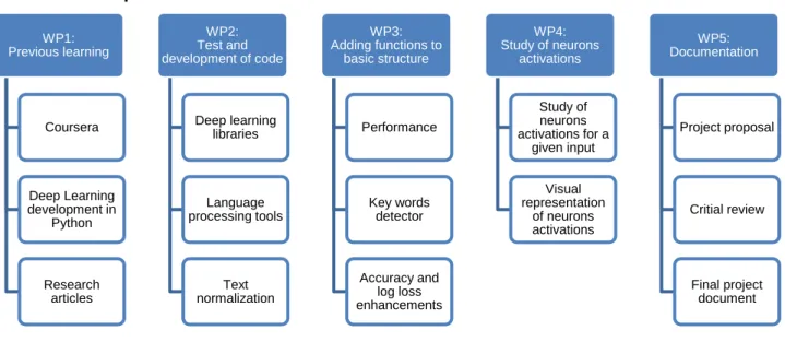
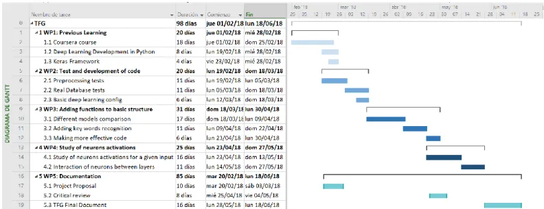
1.4. Work plan, milestones and Gantt diagram 1.4.1. Work plan WP1: Previous learning Coursera Deep Learning development in Python Research articles WP2: Test and development of code Deep learning libraries Language processing tools Text normalization WP3: Adding functions to basic structure Performance Key words detector Accuracy and log loss enhancements WP4: Study of neurons activations Study of neurons activations for a given input Visual representation of neurons activations WP5: Documentation Project proposal Critial review Final project document

(13)

1.4.2. Gantt Diagram

1.4.3. Milestones

WP# Task# Short title Milestone / deliverable Date (week)

2 1 Word embedding x 05/03/2018

2 2 Processing text library

convenience x 05/03/2018

2 3, 4 Deep learning model

convenience x 10/04/2018

3 1, 2, 3 Improved performance of the

definitive model x 23/04/2018

4 1 Study of neurons’ activations

for different category sentences x 23/04/2018

4 3 Extraction of key words using

neurons’ activations on LSTM x 30/04/2017

5 1 Project Proposal Project Proposal document 05/03/2018

5 2 Critical review Critical review document 07/05/2018

5 3 Final Document Final document 02/07/2018

Table 2: Milestones Figure 1: Gantt Diagram

(14)

1.5. Deviations

There have been some modifications regarding the work packages structure compared to the Project Proposal document. On the project proposal, my final intention was to know which words were the most important when classifying the sentence to one category or another. Given that this milestone has already been achieved, long before it was expected, I have added one more work package that represents the continuity of my previous work. Work Package 4, in Project Proposal dedicated to Documentation, has been changed to include all research of the neural network regarding the decision process. For that reason, WP4 includes the study and conclusions of the reaction of the LSTM Layer for a given sentence.

(15)

2. State of the art of the technology used or applied in this

thesis:

This section is intended to create a comprehensive background knowledge that will be useful to understand all topics explained in this thesis. That background includes from the very beginning of artificial intelligence research and results to the last news and improvements on this computer science field. Topics will be treated from the most general to the most specific and technical details.

First, basic knowledge and history of AI and machine learning will be explained and then, deep learning research (specially applied to natural language processing) will be described.

2.1. Artificial Intelligence

Deep learning, which is the technology used in this thesis, is a basic part of a greater concept, machine learning. And thus, Machine Learning comes also from a wider concept, Artificial Intelligence.

Artificial Intelligence (AI) becomes the most general concept when we talk about intelligence machine decisions. It is defined ideally as a rational agent which can provide, by analysing the environment, the best actions to maximise the success probability in a decision-making task.

AI beginnings date back to 1950’s when Alan Turing proposed a test to determine if a machine were indistinguishable from a human being in his article Computing Machinery and Intelligence. But the term “Artificial intelligence” remained unmentioned since the Darmouth Conference in 1956 (John McCarthy).

By 1974, computers were solving algebra word problems, proving theorems in geometry and learning to speak English.

In 1987 Martin Fischles and Oscar Firschein described the necessary attributes for a “intelligent agent”. This spread AI to a wider variety of investigation areas.

In 1997, Deep Blue became the first computer to beat a world chess champion, Garry Kasparov.

In the 2000s decade, chatbots became more human-likely and AI became more powerful due to the huge development in computation power.

The first computer to overcome the Turing test was launched in 2014 (with Eugene program, developed in Russia).

In 2016 a computer powered by a Google’s program beat a world GO champion (a very high complexity and strategy game).

Nowadays, AI has become a daily technology that can be found in autonomous driving cars, virtual reality games, image recognition, language translation…

(16)

2.2. Machine Learning

Machine Learning (ML), a section of computer science and included in the term “AI”, develops the techniques that make possible the process of “learning” for a computer. Furthermore, it is about developing programs which have the ability to infer behaviours and decisions depending on previous provided information.

There are two big categories in machine learning: • Supervised learning

• Unsupervised learning

In supervised learning the samples used to train the computer have more information (labelled samples) whereas non-supervised works without “knowledge” and tries to infer an inner behaviour of samples to look for similarities and differences between them. For instance, if our application is a cat recognition image, we will have to provide train image samples with labels of “cat” or “not cat”. And thus, after training the program, we will have the same output for every input image, “cat” or “not cat”.

Non-supervised learning, however, will have input images without labels, for example, images of all kind of animals. Following the example, non-supervised machine learning will know how to categorize the images by similarity (distinction between animals) but will not know what category corresponds to a “cat”.

For the purpose of this thesis, I will be using supervised learning as I have a labelled database with all training sentences properly classified.

2.3. Deep Learning 2.3.1. Background

Deep learning is a field of computer science, included in the term ML, that studies the ability to learn tasks autonomously from huge quantities of data and information. We can get a pretty accurate description from a Nature article written by Yann LeCun, Yoshua Bengio and Geoffrey Hinton:

“Deep learning allows computational models that are composed of multiple processing layers to learn representations of data with multiple levels of abstraction. These methods have dramatically improved the state-of-the-art in speech recognition, visual object recognition, object detection and many other domains such as drug discovery and genomics. Deep learning discovers intricate structure in large data sets by using the backpropagation algorithm to indicate how a machine should change its internal parameters that are used to compute the representation in each layer from the representation in the previous layer. Deep convolutional nets have brought about breakthroughs in processing images, video, speech and audio, whereas recurrent nets have shone light on sequential data such as text and speech.”

(17)

2.3.2. Neural network basics

Although the process of learning can be computationally difficult if the net is big enough, we can get an overall idea of the process if we review some basic rules of the process:

• A deep neural net is formed by different layers.

• Each neuron has different weights which will be multiplied by the input. • When starting up the neural net, all the weights will be randomly assigned. • The output of the net is the output of the last layer of the net.

• The output will be compared to the “ideal” output (the labels assigned to the input in question) and a loss function will be computed.

• Depending on this loss function, the net is able to change its weights for the next sample to be more accurate.

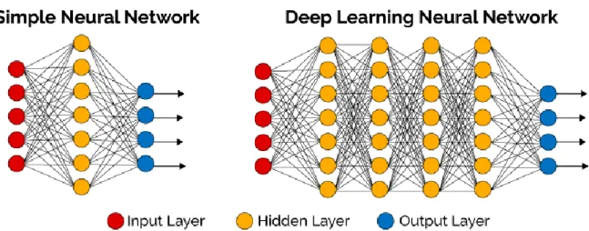
Figure 2: Neural networks diagram with one and four hidden layers

Taken from: https://planetachatbot.com/deep-learning-f%C3%A1cil-con-deepcognition-9af43b2319ba

Input Layer

Input layer will be as long as the training samples on the database. For example, the pixels value of an image, the words of a sentence…

Hidden Layer

Hidden layers have not a determined size. It has to be fixed depending on the accuracy of the performance of the network, so it has to be run every time we want to try its adequacy. Hidden layers can take inputs (from the input layer or from other hidden layers) and multiply its weights by the inputs received. That result will be passed to the next hidden layer or to the output layer if it is the case.

Output Layer

Output layer take its inputs from the last hidden layer and multiplies them by its weights. This layer will output the final decision or behaviour so it has to be the same length as our desired output. In case our neural net has to decide if an image is showing a cat or not, the output layer will only have one node (value 1 for “cat” and 0 for “non-cat”).

Alternatively, if we want to classify sentences into six categories, as it is the case, we will have six nodes at the output layer.

(18)

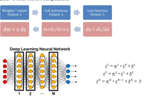
2.3.3. Overall network computations 𝑧1= 𝑤1∗ 𝑥0+ 𝑏1 𝑧2= 𝑤2∗ 𝑥1+ 𝑏2 𝑧𝑁 = 𝑤𝑁∗ 𝑥𝑁−1+ 𝑏𝑁= 𝑦̂ z = outputs w = weights x = inputs b = bias ŷ = predictions

2.3.3.1. Single neuron activations

Each single neuron has a set of weights equal to the number of the inputs of the mentioned neuron plus an extra weight for the bias. These weights, when multiplied by the inputs, assign an importance to every input. The sum of all these multiplications is applied to a function (fNL)such as ReLu, Sigmoid, Tanh, etc. and the activation of the neuron (p̂)

becomes the output of this function.

Weights * inputs

Output: z Cell activationsOutput: a Loss functionOutput: L

dw = x dz

dz=dL/dz=a-y

da = dL/da

Figure 3: Hidden layers enumeration

x1 x2 x3 1 w0 = bias w1 w2 w3

f

NL(y)

(19)

The image above shows a neuron which has 3 inputs and therefore 3 weights. There is another fix input (bias) which in fact can be represented as an input value of 1 multiplied by a desired weight. This is used to adjust the cell activation with a constant factor independent from the input data.

There can be used several activation functions depending on the data we have and the results we want to achieve. For example, if the desired output were a probability, using a sigmoid function on the last layer of neurons will be very recommended as its output range goes from 0 to 1.

2.3.3.2. Loss function

Once we have the outputs of the network for a given input, it has to be some kind of algorithm to evaluate if the performance of the decisions was good enough. This information would help us to change weights’ values to get more accurate results for the next iterations.

The way to conduct this problem in machine learning algorithm is using loss functions. These functions compute the difference between the output of the network for a given input and compares it to the expected ideal output. There are several loss functions, and depending on the application some functions will work better than others.

For classification problems, which is the case in this thesis, there are two widely used loss functions: Mean squared error and Cross entropy loss.

We will use this example table to compute manually these two errors to see the differences between them:

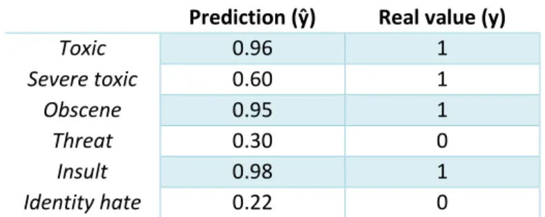
Prediction (ŷ) Real value (y)

Toxic 0.96 1 Severe toxic 0.60 1 Obscene 0.95 1 Threat 0.30 0 Insult 0.98 1 Identity hate 0.22 0

• Mean squared error (MSE):

𝑀𝑆𝐸 ≔ 1

𝑁 ∑(ŷ − y)𝑖

2 𝑁

𝑖=1

Mean squared error computes the square of the difference between predicted and real values of each category and then computes the mean dividing the sum of all of them by the total of categories. For example, given the values in the above table we can compute MSE as:

𝑀𝑆𝐸 ≔ 1 𝑁 ∑(ŷ − y)𝑖 2 𝑁 𝑖=1 =(0.96 − 1) 2_{+ (0.60 − 1)}2_{+ (0.95 − 1)}2_{+ (0.30 − 0)}2_{+ (0.98 − 1)}2_{+ (0.22 − 0)}2 6 = 0.050

(20)

• Cross entropy loss: ℒ(ŷ, 𝑦) ≔ ∑ 𝑦𝑖∗ log 1 ŷ𝑖 𝑖 = − ∑ 𝑦𝑖∗ log ŷ𝑖 𝑖 = −(𝑦 · ln(ŷ) + (1 − 𝑦) · ln(1 − ŷ))

Cross entropy uses the natural logarithm to calculate the loss function. This option is better than MSE in terms of speed during training, so this is the chosen option for the development of the thesis. In this case, the binary cross entropy loss (or log loss) should be computed, as there are only 2 possible real values (0 or 1). Each category shall be predicted independently, giving as a result, a sum of 6 binary cross entropy losses every iteration.

We can compute log loss of a hypothetical last layer with the example values of the table above as:

ℒ1(ŷ, 𝑦) = −(1 ∗ ln(0.96) + (1 − 1) ∗ ln(1 − 0.96)) = −(1 ∗ ln(0.96)) = 0.0408 ℒ2(ŷ, 𝑦) = −(1 ∗ ln(0.60) + (1 − 1) ∗ ln(1 − 0.60)) = −(1 ∗ ln(0.60)) = 0.5108 ℒ3(ŷ, 𝑦) = −(1 ∗ ln(0.95) + (1 − 1) ∗ ln(1 − 0.95)) = −(1 ∗ ln(0.95)) = 0.0512 ℒ4(ŷ, 𝑦) = −(0 ∗ ln(0.30) + (1 − 0) ∗ ln(1 − 0.30)) = −(1 ∗ ln(0.7)) = 0.3567 ℒ5(ŷ, 𝑦) = −(1 ∗ ln(0.98) + (1 − 1) ∗ ln(1 − 0.98)) = −(1 ∗ ln(0.98)) = 0.0202 ℒ6(ŷ, 𝑦) = −(0 ∗ ln(0.22) + (1 − 0) ∗ ln(1 − 0.22)) = −(1 ∗ ln(0.78)) = 0.2485 2.3.3.3. Back-propagation

Back-propagation becomes one of the most important steps in machine learning, as it permits to modify the weights in order to allow the “learning” itself. The loss function mentioned in the previous section, is necessary to perform the derivatives used to fine-tuning the weights.

In sum, this is the formula to update the weights values:

𝑤

_𝑖

≔ 𝑤

_𝑖

− 𝛼 𝑑𝑤

_𝑖

The learning rate 𝛼 means the learning speed, the higher, the fastest. The derivative 𝑑𝑤𝑖=

𝑑ℒ(ŷ,𝑦)

𝑑𝑤_𝑖 means the slope of the loss function with respect to the variable 𝑤𝑖.

To know the value of 𝑑𝑤𝑖 = 𝑑ℒ(ŷ,𝑦)

𝑑𝑤_𝑖 , first other derivatives need to be computed, which will ease the way to extract 𝑑𝑤𝑖. That is why it is named back-propagation, because it is solved step by step backwards.

𝑑𝑎𝑖 = 𝑑ℒ(𝑎, 𝑦) 𝑑𝑎𝑖 = −𝑦 𝑎+ 1 − 𝑦 1 − 𝑎

(21)

𝑑𝑤𝑖 =

𝑑ℒ(𝑎, 𝑦) 𝑑𝑤𝑖

= 𝑥𝑖𝑑𝑧𝑖 = 𝑥𝑖 (𝑎 − 𝑦)

2.3.3.4. Cost function

To control the overall graph performance, we can compute the cost function. The cost function is somehow the indicator that shows how badly a model is predicting some output from a determined input. Therefore, our intention has to be to decrease to the minimum this cost value.

For a determined set of weights, giving determined predictions for a given input, we can extract an exact point of the cost function:

𝐽𝑦(ŷ) = 1 𝑁∑ ℒ𝑖(ŷ, 𝑦) 𝑁 𝑖=0 =1 6∗ 1.2282 = 0.2047

In conclusion, the model has to approach to the weights which minimize the cost function and these transitions has to be slow enough to converge but fast enough to be effective.

2.4. Natural Language Processing

Natural language processing (NLP) is a field of computer science, especially in artificial intelligence, that allows the interaction and understanding of computers of the human language mechanisms.

Natural language can provoke several problems which have been impossible to be solved by a computer not long ago. Some of these cases are:

• Polymorphism: One word can have several and totally different meanings. • References to previous mentioned words.

• Acronyms and slang expressions. • Possible ironical sentences.

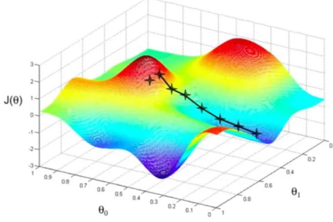
Instead of stablishing a huge number of hard-coded rules, NLP can be effectively implemented on machine learning algorithms by analysing a determined set of samples.

Figure 7: Single weight optimization

Taken from: https://towardsdatascience.com/machine-learning-fundamentals-via-linear-regression-41a5d11f5220

Figure 6: Double weight optimization

(22)

2.5. Framework

All work done in this thesis has to be supported by a software capable of extracting good results and performance. This section will describe the used frameworks regarding the machine learning field. The framework showed has been developed in python.

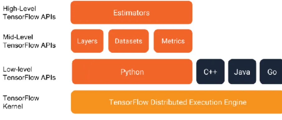
2.5.1. Tensorflow

Tensorflow is an open source machine learning framework developed by Google Brain Team. It is used by companies such as Nvidia, Intel and Qualcomm.

Tensorflow uses data flow graphs to perform complicated numerical tasks. It is distributed in different API layers, going from the easier to modify (estimators) to a Kernel level API.

2.6. Keras

Keras is a high-level neural networks API that uses some frameworks to implement the models. It is capable of running on top of Tensorflow, CNTK or Theano (other deep learning frameworks). It is thought to ease the use of such frameworks, allowing to code models in the same way but enabling the possibility to use different backends. That is the reason it cannot be categorized as a framework, because it is not.

Figure 8: Tensorflow layers diagram

(23)

3. Methodology / project development:

This chapter is aimed to explain in detail the procedures and experiments carried out during the development of this project.

3.1. Database

The database for this project has been collected in Kaggle, concretely in the “Toxic comment classification” competition. This database has three different files:

Train.csv: Contains the raw comments with their respective binary labels.

Test.csv: Contains raw comments, different from the ones in the training dataset. They are not labelled, as the function of this dataset is to predict their labels to “test” the performance of the model.

Test labels: Ideal labels for the test dataset. This data has not been public while the competition was open in order to avoid fraud.

Train.csv Test.csv Test_labels.csv

Samples 159.571 153.164 153.164

Table 4: Number of samples for every category

All samples present in these documents have been extracted from Wikipedia comments, independently from the topic of the article. They are labelled by human ratters and classified, as previously said, within the six following categories:

• Toxic • Severe toxic • Obscene • Threat • Insult • Identity hate

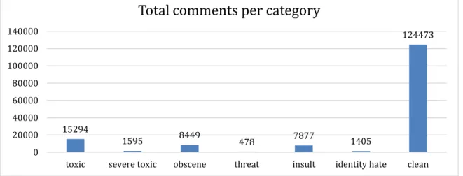
There are less toxic comments than expected, as it can be seen in the next table. This could lead to inaccuracy in some categories of the model, especially in threat comments.

15294 1595 8449 478 7877 1405 124473 0 20000 40000 60000 80000 100000 120000 140000

toxic severe toxic obscene threat insult identity hate clean

Total comments per category

(24)

And so, we can find very kind sentences, or very disgusting comments as well. A csv document prepared to be charged in our model will have the following structure:

“sentence_id”, “comment”, “label_1”, “label_2”, “label_3”, “label_4”, “label_5”, “label_6”

Labels follow the same order as the list of categories above.

3.2. Objectives

It is important to remark the main purposes of this thesis and therefore, the steps this document is going to follow to extract conclusions about the project.

First of all, different model possibilities will be studied and taken into consideration for further investigations. Loss and accuracy will be central indicators of the model performance and adequacy to the database.

Then, using a model from the ones previously characterized, a list of neurons activations will be extracted for every sentence and thus, a quantitative and qualitative importance will be extracted.

To sum up, the overall goal of the project is to create a competitive model for sentence classifying and to be able to see clearly the most important words of an input sentence.

3.3. Key layers for sentence processing

There are a wide variety of methods to process neural networks inputs depending on the data and the results we want to achieve.

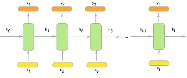
3.3.1. RNN

Recurrent neural networks are thought to perform successfully when applied to sequential input data. That means that it can be effective in natural language processing tasks, as input sentences follow a sequential shape.

Basically, RNN takes any input (a word for example) and extracts an output and a determined weight to make the next word prediction more accurate. That is why RNNs can be seen as multiple feedforward neural networks passing information from one input to the next one.

(25)

Unfortunately, RNNs have an important problem called vanishing gradient problem. It prevents RNNs output to be accurate because are difficult to train. This problem comes from the fact that at each time step during training we are using the same weights to calculate the output. This means that the network experiences difficulty in memorising words from far away in the sequence and makes predictions based on only the most recent ones.

3.3.1.1. GRU

GRU (Gated recurrent unit) is a special kind of RNN, introduced in 2014, which aims to solve the vanishing gradient problem which comes with standard RNNs. To solve this, GRU uses the update and reset gate. What is special about these gates is that they can decide what information should be passed to the output. In fact, they can be trained to keep information from long ago when important or remove it if it is irrelevant for the prediction.

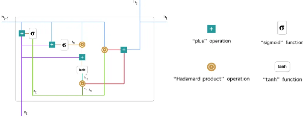
3.3.1.2. LSTM

Long short-term memory networks (LSTM) are a special kind of RNNs designed to be capable of learning long-term dependencies. In fact, it is a more complex version of a GRU cell and it has the same objective: avoiding the vanishing gradient problem.

Figure 13: LSTM operations and internal flow

Taken from: https://codeburst.io/generating-text-using-an-lstm-network-no-libraries-2dff88a3968 Figure 12: GRU gate operations and internal flow

(26)

The key to LSTMs is the cell state, the horizontal line running through the top of the diagram. It is the result of computing the previous cell output by the result of applying some functions to the input.

The first sigmoid layer, ft is to decide what information of the input are we going to throw

away depending on the previous cell. This sigmoid layer is called “forget gate layer”. The next step decides which information is going to be stored in the current cell. That is decided combining a tanh and a sigmoid applied to the input information, then this result is added to the previous cell state.

The final cell output will be ht. It is computed using a tanh of the final cell state (-1, 1) and

another sigmoid of the input (0,1) to force the value to be between -1 and 1 and containing a certain activation.

3.3.2. CNN

For image processing it is widely known the high performance when using convolutional neural networks (CNN). This technique consists in splitting the image in smaller images, subsections of the principal one, in order to enable an easier way to “find” interesting patterns. As an example, if the model is searching for a dog in an image but this dog is in a corner of the image, it may not be spotted when looking at the overall of the picture but it will be found when looking in smaller subsections.

Given this information, it may seem that CNNs are not a good choice for natural language processing and sentence classification. That is incorrect, as it has performed incredibly well as the core part of one of the developed models which will be demonstrated on the following pages. It can be though that convolutional neural networks can be a pretty accurate solution if we realize that images can be represented, in fact, in the same way of a sentence, as an array of numbers.

As we can see, an image can be represented with a set of numbers, representing the value of black in this example. This can be represented as an array of numbers:

Figure 14: Example of pixel representation on a basic image

Taken from: https://medium.com/@ageitgey/machine-learning-is-fun-part-3-deep-learning-and-convolutional-neural-networks-f40359318721

(27)

Figure 15: Similarity between image pixels representation and tokenized sentences

Taken from: https://medium.com/@ageitgey/machine-learning-is-fun-part-3-deep-learning-and-convolutional-neural-networks-f40359318721

3.4. Development environment and tools

After having seen the main key layers used in tasks such as natural language processing or image recognition, it is necessary to study the relationship between theory and practise. It is time to start to see how a neural net can be implemented in a software environment. For this project, I chose to use the TensorFlow framework for its well-known importance in the machine learning industry. To ease the development of the code and framework usage, the code will work with the Keras API.

3.5. Model development

The aim of this section is to clearly explain how a neural net can be implemented using the Keras API with a backend working with TensorFlow. This section also includes the web development which receives, processes and presents the ML computation results.

3.5.1. Text pre-processing

It is highly recommended on natural language processing the treatment of texts before analysing them in the neural network. This is achieved by replacing an original word by a more general word without losing meaning. Theoretically, there are several benefits on the model results if the texts are cleaned before processed. For example, some of the key actions that are usually carried out in pre-processing are:

• Stemming: Convert all the verb conjugations into the root verb.

• Plural to singular: Depending on the application, converting plural to singular nouns will not cause a lack of meaning but an increased performance.

• Erasing symbols: Words followed by symbols will be treated as different when, in fact, they have the same meaning. Example:

In the project, the first two actions are carried out using the methods inside “preprocessing.py”: “sentence_to_words” for extracting singular words out of sentences and “lemmatize” for stemming and avoiding plural words.

3.5.2. Model creation

Once we have the dataset prepared, either pre-processed or not, it is time to start building the model. It is important to know that all the proposed models have been thought to both increase the performance at the maximum and to be able to extract information regarding the decisions the network is taking.

3.5.2.1. Input length

One of the first decisions to be made is the input length of the network. It has to be a fixed value, and at the same time it is known that every sentence has different length. For this reason, comments exceeding the input length will have to be truncated and the ones

(28)

shorter than the input length will have to be filled with dummy values. This input length value has been stablished in 200 words per comment after computing a histogram with all the comments length. The decided length does not respond to a clear decision, as nothing states that this value will work better than other before training time.

3.5.2.2. Tokenizer

In section 3.3.2 CNN it was demonstrated how an image could be transformed into an array of numbers prepared to be entered directly in a network. Unfortunately, in NLP it is not as intuitive as image processing in this case.

Words can also be represented as numbers. One easy way of representing them will be to assign a number every time a new word appears and use this number instead of the word if it is being used again. Another method will be using lower numbers for words appearing with a higher frequency.

For this purpose, in this thesis has been used the predetermined Tokenizer that comes with Keras. It uses the second method explained above: assigns numbers to words depending on their frequency. This Tokenizer includes some arguments to add more functionality, two of them are important for the models:

• Num_words: Only the most common num_words will be kept. • Filters: List of symbols to be erased from the saved words.

Num of words is set to 20.000 to avoid possible lack of memory to keep new words. Filters are part of the 3.5.1 section, pre-processing, but will not be used in Keras Tokenizer, as they are extracted using regex package in token_extraction.py. Tokenizer also extracts punctuation by default.

The usage of this tool requires, first, a “dictionary training” to link every of the 20.000 numbers to words using the training dataset. Then, sentences in test.csv will be tokenized following the relationships fixed during training

Example of a sentence from test.csv dataset with invented tokens:

I WILL BURN YOU TO HELL IF YOU REVOKE MY TALK PAGE ACCESS

After that, we have to run “pad_sequences” from sequences.py, another Keras module to adjust the length as explained in the previous section.

14 591 892 12 20 5622 401 12 7898 78 2013 3029 1887

1 2 3 4 5 6 7 8 9 10 11 12 13 14 15 … 199 200

14 591 892 12 20 5622 401 12 7898 78 2013 3029 1887 0 0 … 0 0

Table 5: Possible representation of a tokenized sentence

"I WILL BURN YOU TO HELL IF YOU REVOKE MY TALK PAGE ACCESS!!!!!!!!!!!!!"

(29)

3.5.2.3. Embedding

After tokenizing train and test comments, the program is able to introduce the information to the network. The first stage once inside the network is the Embedding layer. This layer receives the input, the sentence, and outputs a vectorized representation of every word of personalized length.

This is important to represent every word in a N-dims space, where words will be placed closely to other similar words.

Let’s imagine a situation where words are labelled as explained in section 3.5.2.2.

The inner product between all words is 0. That means there are not relationships nor dependencies between them. For instance, taking this example:

I want a glass of orange _________. I want a glass of apple ___________.

Both sentences should have the same output, “juice”. And both sentences could be treated as one if orange and apple were closely represented.

• Featured representation:

Man (5391) Woman (9853) King (4914) Queen (7157) Apple (416) Orange (6257)

Figure 16: Sentence embedding diagram and input preparationMan (5391) Woman (9853) King (4914) Queen (7157) Apple (416) Orange (6257)

(30)

3.5.2.4. Feature extraction and classification network

Taking into account that it is needed a layer to obtain a good performance on NLP, the options used for this project have been GRU, LSTM and CNN. The three performances and results have been computed and they are published on the section 4.

The LSTM model is based on the one presented by Mireia Gartzia, Carlos Arenas and Itziar Sagastiberri which was made for the same toxic comment competition. In this model, the aim is to add some enhancements and introduce the cell activation extraction. This model is composed of 60 LSTM cells and a posterior layer of GlobalMaxPooling1D to reduce the dimensionality of the samples from 3D (words, embedding, samples) in LSTM to 2D (highest embedding value, samples) in MaxPooling.

The GRU model has been created to compare a similar approach to the LSTM model in performance and in efficiency. GRU model does not include cell activations and also consists in 60 GRU cells and GlobalMaxPooling to make possible a fair comparison with LSTM.

The CNN model has been developed to compare a totally different approach from the other two models. CNN model does not include cell activations. It is composed of two convolutional layers in parallel with filter sizes of length 3 and 5. Then, the two layers go through a MaxPooling1D and at the end the layers are concatenated. MaxPooling1D is different from GlobalMaxPooling1D because it does not reduce dimensionality but downsamples its inputs.

To finish the network, it is necessary to end with a layer of length 6, as the categories of toxicity. For this reason, it is highly recommended to end the graph with some normal layers called “Dense”. There is an exception in the CNN model, where it is placed another

Figure 18: LSTM model flow chart for 1 sample

(31)

3.5.2.5. Hyperparameters

Hyperparameters are manual adjustable parameters to fit the model depending on the database, the computer performance, the problem faced… This project was not intended to compare performances with different hyperparameters, so there is an enumeration of the most important ones, but there is not a hyperparameter tuning. These parameters have been chosen for being a usual choice in similar networks for NLP so it is expected to have a good performance for the development of the rest of the project which is the extraction of activations and a comparison between CNN, GRU and LSTM models.

Some of the hyperparameters used are: • Batch size: 32

Number of sentences to be propagated through the network before updating weights.

• Optimizer: Adam

It is needed to compute the loss and update the weights every batch_size samples. It includes the learning rate as a parameter.

• Learning rate: 0.001

The learning rate 𝛼 means the learning speed, the higher, the fastest. Explained in section 2.3.3.3.

(32)

• Epochs: 2

The number of times a complete dataset is passed through the network to train the weights. Too many times can overfit the network (adjusting too much the training for the training samples) and low values can cause underfitting which is the lack of training on a model.

3.5.3. Activations extraction

One of the first objectives and reasons to do this project was to see if it was possible to extract any conclusion about the network decisions and therefore, its activations. What were the most important words? Which one of them made the network made a choice or another?

To make this happen, a script extracts all layers in a model and applies them an input. It evaluates model and extracts its activations when the input goes through it. In fact, the objective is to zoom what is happening at the end of the 60-nodes LSTM layer, and it is expected to observe a greater activation value on most of the neurons when a toxic word goes through them.

This feature must not be confused with attention mechanisms, which aim to enhance the network performance. Activations extraction has only a visualizing purpose and understanding of the net and will not impact on the final accuracy, as it is run with the model weights already saved.

3.5.4. Web representation

To provide a visual and easy to use environment, this project also includes the development of a web page to show the results extracted from the machine learning scripts. It is a very basic web with only a title, a textbox to enter any test sentence and a results section.

The aim of this section is to show more visual results and to learn how to provide quickly results using pre-charged trained networks as well as pre-charged tokenizers. This section is intended to be just a help to understand all the results achieved from now on.

It is fully developed in the Python web framework Django and interacts with the same scripts made for terminal, although there have been some modifications to adapt it for the HTML and CSS needs.

(33)

4. Results

This chapter includes the results obtained in the three different tested models. This will make possible to compare them in the same conditions and then, choose what is best for the project’s necessity. It is important to highlight that performance results will not change the fact that activations study will be based in the LSTM model as well as the web server.

4.1. Pre-processed vs not processed sentences

These are charts representing the training loss in front of the validation loss. This is useful to find the maximum epoch that will be beneficious to the model. Overfitting is defined as the training loss being lower than validation loss, that tells us that the model has over-trained and has very accurate results for the training database but worst results when testing. The best epoch will be determined by the intersection of the two losses.

The charts represent the loss value on the three total epochs (0, 1 and 2) for each model without pre-processing. As it can be easily seen, the best value for the total epochs is two, as it is the nearest value to the intersection. One epoch will mean underfitting and three epochs will cause overfitting. Normally, for a smaller database it will be necessary to run more epochs to train the model.

The following table shows performance for every of the three models, including log loss and accuracy and 2 epochs without pre-processing.

Table 6: Comparison of performance in CNN, LSTM and GRU models. Without preprocessing. The three models present a very similar accuracy and loss after training, but the convolutional model stands out in processing time. This similarity is probably caused by the big database provided. For the web implementation the best option, in my opinion, will

Convolutional GRU LSTM

Convolutional LSTM GRU

Log loss Accuracy Log loss Accuracy Log loss Accuracy 1st epoch 0.0525 0.9808 0.0500 0.9778 0.0486 0.9760 2nd epoch 0.0505 0.9816 0.0477 0.9832 0.0468 0.9834

Time 770s/epoch 1208s/epoch 1120s/epoch

(34)

be to use the convolutional model, as the response time will be half of the others. To extract conclusions about the decisions, the perfect model will be the LSTM for the relationship with NLP implementations and the more complex structure compared to the GRU model. The results of the same models applying pre-processing and maintaining the same number of epochs are:

Compared to the results obtained in the not pre-processed models, it can be concluded that pre-processing sentences does not represent a clear gaining in loss nor in accuracy. The LSTM is getting better results in loss but worst in accuracy when using pre-processed sentences, but GRU achieves worst results in loss and accuracy. The convolutional model seems to be working a little better with pre-processed sentences.

It is important to remark that these changes are very small and cannot be treated as an enhancement or loss of accuracy. Moreover, pre-processed models last almost twice as the not pre-processed models although this extra time is not included in the above table because pre-processing happens before the model is run.

4.2. Neuron’s activations

Using pyplot, the results of the activation for a toxic sentence are:

There can be easily distinguished the higher values, corresponding to higher activations, thus, more importance. The Y axis is representing the 60 neurons whereas X axis represents the input sentence word by word. If we pay attention to, for example, the seccond word, we could see that it presents, on average, higher values on its neurons (see vertically). This occurrence coincides with the fact that the second word is an insult “bitch”, and then, a very important word for the categorization of the sentence.

It happens the same with the word “hating”, “bitch” (another time) and “pathetic”, they all obtain high activation values at the output of

Convolutional LSTM GRU

Log loss Accuracy Log loss Accuracy Log loss Accuracy 1st epoch 0.0533 0.9807 0.0502 0.9814 0.0508 0.9815 2nd epoch 0.0503 0.9819 0.0471 0.9823 0.0483 0.9815

Time 710s/epoch 1215s/epoch 1057s/epoch

(35)

4.3. Web visualization

This section shows an example of the representation seen in the developed web page. It can be seen as activations and classifications are now mixed and well presented for a quick and intuitive visualization.

Figure 25: Django web page displaying the importance of singular words and results for a toxic sentence

Figure 26: LSTM activations for a toxic sentenceFigure 27: Django web page displaying the importance of singular words and results for a toxic sentence

(36)

5. Budget

This thesis does not consist in the realization of any prototype, so there will not be any kind of material costs. In fact, the only cost consists in a computer and a human cost in hours taking into account a junior fee and a supervisor fee.

This project started on February 2018, what makes it a total of 21 weeks until July 2018, at a mean of 25 hours per week gives a total of 525 hours approximately. Taking into account that the fee for a junior engineer will be about 10€/h, the cost of a junior engineer to make this project will be 5250€.

It is important to remark the importance of the supervisor in this kind of project so it is a fact that he or she will have to receive a salary as well. A salary of 80€/h is fair compared to the cost of hiring a senior with this experience, and the hours dedicated are calculated taking into account meetings of 1 hour every two weeks starting one month after the start of the project (8 meetings more or less). The total amount will be 160€.

Regarding the technology used, a computer with enough power to run correctly the scripts can cost about 700€ and it has been used for half a year. The amortization percentage has been consulted using the percentages of agencia tributaria. The project has been developed using Keras which is a free library and the software editor Visual Studio Code which is also free.

Price Cost Junior 10€/h * 525h 5250€ Supervisor 80€/h * 8h 640€ Electronic devices amortization [25%*700€] * 0.5y 87.5€ per 6 months TOTAL 5977.5€

(37)

6. Conclusions and future development:

Several goals have been achieved during the realization of this thesis. The first and most important one is the acquisition of fundamental knowledge and background of neural networks computations. This stablishes a good basis to develop more skills in the future and self-improvement.

Regarding practical results, it has been stated and proved that the LSTM model has achieved a high accuracy in sentence classification, which was the main problem that was faced in this project. Regarding pre-processing, it has to be said that it was expected to obtain substantially better results when training under a pre-processing environment, but it turned to be false, the results happened to be almost the same.

Once accomplished that, the aim of the thesis was to present and analyse the performance of different models in this sentence classification.

The three choices result in an outstanding performance, so much so that the three options present very similar results. It may be caused by the huge size of the database and then, the facility for all models to adjust its weights with so many samples.

Unfortunately, it is important to state that the threat category has not performed as well as the other. This can be caused for the small number of threat training sentences (478 out of a total of 159.571).

The most challenging objective of this thesis, and what makes it personal and different is the ability to extract valuable information out of the neural network cells. This feature has been focused only on the LSTM model because it was the most intuitive one in terms of internal behaviour. It has been successfully achieved and adapted to be shown more intuitively in a web page.

Also, this project included a part of web development in Django, although it did not take a principal importance in the development of the thesis. It only helped to show clearer results, which was one of the objectives since the very beginning of the project.

One important aspect explained during the project is the ability of convolutional neural networks to have good performance natural language processing problems. At first, this kind of network did not seem a choice for this problem since it is mainly used in video and image processing. This feature has been reviewed and confirmed explaining the similarities between the representation of images and sentences.

In general, this thesis has made possible for me to dive in the insights of a neural network, understanding how these decisions are taken and being able to represent it in a very visual way. All this work is thought to bring a field of AI closer to non-technical people, making explanations as simpler as possible but technical when required.

It is slightly difficult to propose future implementations using this project since it has achieved all the goals proposed at the beginning. It may be interesting to go a little bit further and see step by step computations made by the LSTM, CNN and GRU. Another idea would be to use the activations to somehow increase the model performance, as an attention layer.

(38)

Bibliography:

[1] Lecun, Y., Bengio, Y., & Hinton, G. (2015). Deep learning. Nature, 521(7553), 436–444. https://doi.org/10.1038/nature14539

[2] Yang, Z., Yang, D., Dyer, C., He, X., Smola, A., & Hovy, E. (2016). Hierarchical Attention Networks for Document Classification. Proceedings of the 2016 Conference of the North American Chapter of the Association for Computational Linguistics: Human Language Technologies, 1480–1489.

https://doi.org/10.18653/v1/N16-1174

[3] Srivastava, N., Hinton, G., Krizhevsky, A., Sutskever, I., & Salakhutdinov, R. (2014). Dropout: A Simple Way to Prevent Neural Networks from Overfitting. Journal of Machine Learning Research, 15, 1929–1958.

https://doi.org/10.1214/12-AOS1000

[4] Kim, Y. (2014). Convolutional Neural Networks for Sentence Classification. https://doi.org/10.3115/v1/D14-1181 [5] Andrej Karpathy. “The Unreasonable Effectiveness of Recurrent Neural Networks”. 21 May 2015

https://karpathy.github.io/2015/05/21/rnn-effectiveness/ [6] Edwin Chen. “Exploring LSTMs”.

http://blog.echen.me/2017/05/30/exploring-lstms/

[7] Jason Brownlee. “Understand the Difference Between Return Sequences and Return States for LSTMs in Keras”. 24 october 2017.

https://machinelearningmastery.com/return-sequences-and-return-states-for-lstms-in-keras/ [8] “Understanding LSTM Networks”. 27 August 2015.

http://colah.github.io/posts/2015-08-Understanding-LSTMs/ [9] Phillipe Remy. “Extract the activation maps of your Keras models”.

https://github.com/philipperemy/keras-visualize-activations

[10] Jason Brownlee. “How to Use Word Embedding Layers for Deep Learning with Keras”. 4 October 2017.

https://machinelearningmastery.com/use-word-embedding-layers-deep-learning-keras/

[11] Jason Brownlee. “How to Diagnose Overfitting and Underfitting of LSTM Models”. 1 September 2017.

https://machinelearningmastery.com/use-word-embedding-layers-deep-learning-keras/ [12] Google Developers. Chart Gallery.

https://developers.google.com/chart/interactive/docs/gallery/

[13] Apoorva Agrawal. “Loss Functions and Optimization Algorithms. Demystified.”. 29 September 2017.

https://medium.com/data-science-group-iitr/loss-functions-and-optimization-algorithms-demystified-bb92daff331c

[14] Denny Britz. “Understanding Convolutional Neural Networks for NLP”. 7 November 2015.

http://www.wildml.com/2015/11/understanding-convolutional-neural-networks-for-nlp/ [15] TensorFlow. “Convolutional Neural Networks”. 25 May 2018.

http://www.tensorflow.org/tutorials/mnist/beginners/index.md

[16] Simeon Kostadinov. “Understanding GRU networks”. 16 December 2017.

https://towardsdatascience.com/understanding-gru-networks-2ef37df6c9be

[17] Adam Geitgey. “Machine Learning is Fun! Part 3: Deep Learning and Convolutional Neural Networks”. 13 June 2016.

(39)

Appendices:

Convolutional model:

(40)

LSTM model:

Sentence tokenizer with pre-processing module:

(41)

Glossary

A list of all acronyms and the meaning they stand for. LSTM: Long-Short Term Memory

GRU: Gated recurrent unit

CNN: Convolutional neural network RNN: Recurrent neural network NLP: Natural language processing API: Application programming interface AI: Artificial Intelligence