AUTOMATIC ICE THICKNESS ESTIMATION IN RADAR IMAGERY BASED ON CHARGED PARTICLES CONCEPT

AUTOMATIC ICE THICKNESS ESTIMATION IN RADAR IMAGERY BASED ON

CHARGED PARTICLES CONCEPT

Maryam Rahnemoonfar

, Member, IEEE, Amin Abbasi Habashi

, John Paden

, Geoffrey C. Fox

1.

Department of Computing Sciences, Texas A&M University-Corpus Christi, Corpus Christi, TX

2.

Department of Surveying Engineering, University of Isfahan

3.

Center for Remote Sensing of Ice Sheets, University of Kansas, Lawrence, KS

4.

School of Informatics and Computing, Indiana University, Bloomington, IN

ABSTRACT

Accelerated loss of ice from Greenland and Antarctica has been observed in recent decades. Ice thickness is a key factor in making predictions about the future of massive ice reservoirs and can be estimated by calculating the exact location of the ice surface and bottom in radar imagery. Identifying the locations of ice boundaries is typically performed manually which is a very time consuming procedure. Here we propose a novel approach which automatically detects the complex topology of ice surface and bottom boundaries based on charged particle concept. Here we first applied anisotropic diffusion to remove the noise and enhance the image. At the second step, we detected the contours in the image based on Coulomb's electrostatic law and the assumption that each pixel is an electrically charged particle. The final ice surface and bottom are detected based on the projection profile of the contours. The results are evaluated on a large dataset of airborne radar imagery collected during IceBridge mission over Antarctica and show promising results with respect to hand-labeled ground truth.

Index Terms—Remote sensing, image analysis,

radar

1. INTRODUCTION

Thus far, serious damages have been caused to our environment by global warming. In recent decades, accelerated loss of ice from Greenland and Antarctica has been observed [1]. The melting of polar ice sheets and mountain glaciers, potentially leading to the flooding of coastal regions and putting millions of people around the world at risk, has a significant influence on sea level rise and ocean currents. Precise calculation of ice thickness therefore is very important for sea level and flood monitoring. Usually, human experts in order to identify ice and bedrock, mark ice sheet layer and bedrock by hand, which is a very time consuming and tiresome task and may create errors. To provide important information about ice sheet thickness, the multichannel coherent radar depth sounder was used during the IceBridge mission [2]. In this work the images are the CReSIS standard output product [3] and by using

pulse compression, synthetic aperture radar (SAR) processing, and multi-looking they are formed. The complete processing details are provided in Gogineni et al. [4].

For layer finding and ice thickness in radar images, several semi-automated and automated methods have been introduced in the literature [5] [6][7][8][9]. Crandall et al [5] used probabilistic graphical models for detecting ice layer boundary in echogram images. The extension of this work was presented in [6] where they used Markov-Chain Monte Carlo to sample from the joint distribution over all possible layers conditioned on an image. A Gibbs sampling instead of dynamic programming based solver was used for performing inference. The problem with using graphical models is that it needs a lot of training samples (around half of the actual dataset) which can be very time-consuming to be labeled manually by a human. In another work, Gifford [7] compared the performance of two methods, edge based and active contour, for automating the task of estimating polar ice and bedrock layers from airborne radar data acquired over Greenland and Antarctica. They showed that their edge-based approach offers faster processing but suffers from lack of continuity and smoothness that active contour provides. Mitchell et al [8] used a level set technique for estimating bedrock and surface layers. However, for each single image the user needs to re-initialize the curve manually and as a result the method is quite slow and was applied only to a small dataset. This problem was fixed in [9] where authors introduced a distance regularization term in the level set approach to maintain the the regularity of level set intrinsically. Therefore, it does not need any manual re-initialization and was automatically applied on a large dataset.

result for each pixel is bound to count as edges of image. To improve the quality of counter detection, the images were first enhanced by anisotropic diffusion [10] and the final layers were results for calculating the local maxima in the projection profile.

After this introduction, the details of the proposed method will be discussed in section 2. Experimental results will be discussed in section 3. The results are evaluated in section 4.

2. METHODOLOGY

Our method consists of three main steps:1- anisotropic diffusion to remove the noise and enhance the quality of the image while preserving the edges. 2- ElFi method which is our proposed contour detection algorithm based on the theory of electrostatic and 3- projection profile to extract the layers of ice surface and bottom from the output of contour image.

2.1. Anisotropic Diffusion

Radar imagery suffers from low signal to interference and noise ratios (SINR) due to a) signal attenuation while traveling through ice, b) radar clutter energy, and c) thermal noise and occasional electromagnetic interference. It is necessary to remove noise prior to any contour detection algorithm. However most of the enhancing techniques, in addition to removing noise will affect the quality of edges and contours. Here we used anisotropic diffusion technique [10] which remove the noise effect while preserving the contour’s quality.

In the diffusion equation, the diffusion coefficient c is considered as a constant independent of the space location. The anisotropic diffusion equation is:

� 𝐼𝐼𝑡𝑡=𝑑𝑑𝑑𝑑𝑑𝑑(𝑐𝑐(𝑥𝑥,𝑦𝑦,𝑡𝑡)∇𝐼𝐼)

𝐼𝐼𝑡𝑡=𝑐𝑐(𝑥𝑥,𝑦𝑦,𝑡𝑡)∆𝐼𝐼+∇𝑐𝑐.∇𝐼𝐼 (1)

where div is divergence operator, ∇ is the gradient operator and ∆is the Laplacian operator. if we presume

c (x, y, t) as a constant, the isotropic heat diffusion

equation will be:

𝐼𝐼𝑡𝑡=𝑐𝑐∆𝐼𝐼 (2)

Later, this method undergone smoothing filter withina region in preference to smoothing acrossthe boundaries by setting the conduction coefficient in the interior to be 1 and 0 at the boundaries of each region. Therefore, the blurring occurs separately in each region with no interaction between regions, which these region boundaries would remain sharp.

2.2. ElFi Method

To detect the boundary of ice surface and bottom layers, we developed a novel contour detection technique based on electric field (ElFi). Most of the pioneering methods

in contour detection are based on quantifying the presence of a boundary at a given location in the image. The Roberts, Sobel, and Prewitt operators detect edges by convolving an image with given operators. The Canny method [11] uses non-maximum suppression and hysteresis thresholding steps to model sharp discontinuities in a given image. Moreover, there are several unique and novel researches on edge detection methodologies so far. As an example, the method used in [12] is based on theory of universal gravity to perform edge detection. Therefore, as an inspiration, we used Coulomb's Law of electrostatic force to extract the image contours. It is believed that having both attractive and repulsive forces as a unique characteristic of charged particles will improve the contour detection performance in images.

In the ElFi method, every pixel is assumed to be an electrically charged particle that has electrostatic interaction with other neighboring particles. Initially, by comparing the pixel characteristic with particle characteristic, it can be seen that each particle in the real world has two characteristics: firstly, it has a small charge; secondly, the charge can be positive or negative. The pixel values in grey level image vary between 0 and 255 and they are always positive value. Therefore, in the first step, pixel values will be transferred to a range more similar to electrically charged particles according to equation 3:

𝑞𝑞𝑖𝑖=2𝑝𝑝𝑖𝑖−2 𝑛𝑛_{+ 1}

2𝑛𝑛+1₋₁ (3)

where 𝑝𝑝_𝑖𝑖 is the grey level value of pixel i and 𝑞𝑞_𝑖𝑖 is the equivalent electrical charge for that pixel. n is the number of bits in the image.

Then, the both force types, be it attractive or repulsive, specifies the electric field direction used for contour detection. The electric field of a point charge, which is located in the center, can be obtained from Coulomb's law:

𝐸𝐸�⃑1=_𝑞𝑞𝐹𝐹⃑ 1

(4)

where 𝐸𝐸�⃑₁ is electric field of 𝑞𝑞₁ particle affected by surrounding particles in the 𝑞𝑞₁ neighborhood.

This equation is computed for every neighbor of central pixel. The differential electric field for two neighbor particles is calculated according to equation 5:

∆𝐸𝐸𝑖𝑖(𝑄𝑄𝑖𝑖) =|𝑄𝑄𝑖𝑖_|𝑟𝑟− 𝑞𝑞1| 𝑖𝑖|2

𝑟𝑟⃑𝑖𝑖 |𝑟𝑟𝑖𝑖|

(5)

where 𝑄𝑄_𝑖𝑖 is the electric charge of the neighbor i and𝑞𝑞₁ is the electric charge of central pixel. Finally, the vector sum of all electrical fields is used to calculate the magnitude of signal variation and to detect image contours. For example, for a 3*3 kernel in the image, the equation 5 would be in the following form:

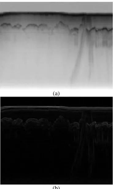
Figure 1b shows the result of applying the ElFi technique on the enhanced SAR image ( Figure 1a) where the top layer is the ice surface and bottom layer is the ice bottom which can be a bedrock or sea surface.

(a)

(b)

Figure 1: (a) Enhanced SAR image by Anisotropic diffusion, (b) the result of ElFi technique

2.3. Projection profile

As it can be seen in figure 1b the image contours are highlighted where the ice surface and bottom have brighter values. To extract the exact ice surface and bottom boundaries, we calculated the the local horizontal projection profile on every 5 pixels’ column. The two local maximum in the projection profile (Figure 2) depicts the location of ice surface and bedrock.

Figure 2: Horizontal projection profile for local vertical columns

3. EXPERIMENTAL RESULTS

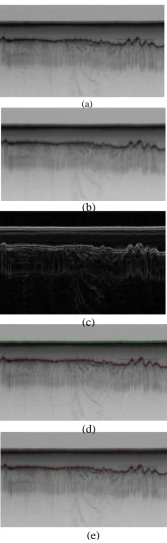
We applied the proposed approach on the 2009 NASA Operation IceBridge Mission. The images have a resolution of 900 pixels in the horizontal direction, which covers around 50km on the ground, and 700 pixels in the vertical direction, which corresponds to 0 to 4km of ice thickness. We applied our method on total of 323 images and compared the results with the ground truth. The ground-truth images have been produced by human annotators. Figure 3 shows the results of our approach with respect to the ground-truth. Figure 3a shows the original image. Figure 3b shows the result after anisotropic diffusion. As it can be seen in this figure, the image is enhanced while the edges are preserved. This stage is necessary for reducing the noise. At the next step, the ElFi method was applied on the enhanced image. As it can be seen in figure 3c, ElFi method detects contours in the image. To highlight the ice surface and bottom boundaries, the projection profile of the ElFi result was calculated. Figure 3d shows our final results. Figure 3e shows the ground-truth results acquired by manually picked layers. The output of our approach shows a satisfactory results compared to the manually picked interfaces.

To evaluate the performance of our approach, we calculated precision (P), recall (R), and F-measure as follow:

R =_{Tp + FN}Tp (7)

P =_{TP + FP}TP (8)

where TP is true positive or correct result, FP is false positive or unexpected result, FN is false negative or

Vertical edge of the image

P

ixe

ls

c

missing results, and TN is true negative. Precision measures the exactness of a classifier and recall measures the completeness of a classifier. They can be combined to produce a single metric known asF-measure, which is the weighted harmonic mean of precision and recall. The F-measure defined as:

F = 1

𝛼𝛼_𝑃𝑃1+ (1− 𝛼𝛼) 1_𝑅𝑅 (9)

captures the precision and recall tradeoff. The F-measure is valued between 0 and 1, where larger values are more desirable.

Table 1 shows the average precision, recall and F-measure on our entire dataset.

Table 1: The result of our approach on 2009 NASA Operation IceBridge Mission

Precision Recall F-measure Our results 0.84 0.79 0.81

Figure 3: The result of our approach. a) original image, b) the enhanced image after anisotropic diffusion, c) detected contours with ElFi technique, d) detected ice surface and bottom after projection profile, e) ground-truth

4. CONCLUSION

In tis paper we developed a novel approach which automatically detects the complex topology of ice surface and bottom boundaries based on Electric field (ElFi). Here we first applied anisotropic diffusion to nd

(b)

(c)

(d)

enhance the image while preserving the edges. At the second step, the contours were detected based on Coulomb's electrostatic law and the assumption that each pixel is an electrically charged particle. The final ice surface and bottom were detected based on the projection profile of the contours. The results were evaluated on a large dataset of airborne radar imagery collected during IceBridge mission over Antarctica and we reached high accuracy of 81% with respect to hand-labeled ground truth.

5. REFERENCES

[1] A. Shepherd et al., “A reconciled estimate of ice-sheet mass balance (vol 57, pg 88, 2010),” Science, vol. 338, no. 6114, pp. 1539–1539, 2012.

[2] C. Allen, L. Shi, R. Hale, C. Leuschen, J. Paden, B. Pazer, E. Arnold, W. Blake, F. Rodriguez-Morales, and J. Ledford, “Antarctic ice depth-sounding radar instrumentation for the nasa dc-8,” Aerospace and Electronic Systems Magazine, IEEE, vol. 27, no. 3, pp. 4–20, 2012.

[3] C. Leuschen, “Icebridge snow radar l1b geo-located radar echo strength profiles,” Boulder, Colorado, NASA DAAC at the National Snow and Ice Data Center, do i, vol. 10, 2013.

[4] S. Gogineni, J.-B. Yan, J. Paden, C. Leuschen, J. Li, F. Rodriguez-Morales, D. Braaten, K. Purdon, Z. Wang, and W. Liu, “Bed topography of jakobshavn isbr, Greenland, and Byrd glacier, Antarctica,” Journal of Glaciology, vol. 60, no. 223, pp. 813–833, 2014. [5] D. J. Crandall, G. C. Fox, and J. D. Paden, “Layer finding in radar echograms using probabilistic graphical models,” in Pattern Recognition (ICPR), 21st International Conference on, 2012, Conference Proceedings.

[6] S.-R. Lee, J. Mitchell, D. J. Crandall, and G. C. Fox,“Estimating bedrock and surface layer boundaries and confidence intervals in ice sheet radar imagery using mcmc,” in Image Processing (ICIP), 2014 IEEE International Conference on. IEEE, Conference Proceedings, pp. 111–115.

[7] C. M. Gifford, G. Finyom, M. Jefferson Jr, M. Reid, E. L. Akers, and A. Agah, “Automated polar ice thickness estimation from radar imagery,” Image Processing, IEEE Transactions on, vol. 19, no. 9, pp. 2456–2469, 2010.

[8] J. E. Mitchell, D. J. Crandall, G. C. Fox, M. Rahnemoonfar, and J. D. Paden, “A semi-automatic approach for estimating bedrock and surface layers from multichannel coherent radar depth sounder imagery,” in SPIE Remote Sensing. International Society for Optics and Photonics, Conference Proceedings, pp. 88 921–88 926.

[9] M.Rahnemoonfar, M. Yari, G.C. Fox, Automatic polar ice thickness estimation from SAR imagery, Proc. SPIE, Radar Sensor Technology XX, 982902

[10] P. Perona and J. Malik, Scale-Space and Edge Detection Using Anisotropic Diffusion, IEEE

Transactions on Pattern Analysis and Machine Intelligence, 12(7):629-639, July 1990

[11] Canny, J.: ‘A computational approach to edge detection’, Pattern Analysis and Machine Intelligence, IEEE Transactions on, 1986, (6)