Towards an Understanding of Facets and Exemplars of Big Data Applications
Geoffrey C.Fox1, Shantenu Jha2, Judy Qiu1, Andre Luckow2
(1) School of Informatics and Computing, Indiana University, Bloomington, IN 47408, USA,
(2) RADICAL, Rutgers University, Piscataway, NJ 08854, USA
Abstract
We study many Big Data applications from a variety of research and commercial areas and suggest a set of characteristic features and possible kernel benchmarks that stress those features for data analytics. We draw conclusions for the hardware and software architectures that are suggested by this analysis.
1. Introduction
With the proliferation of data intensive applications, there is a critical and timely need to understand these properties and the relationship between different applications. The aim of our work is to capture the essential and fundamental Big Data properties, and then to understand applications with those properties.
There are many different types of Big Data applications, and we cover them broadly including both research and commercial cases. However our focus is on Science and Engineering research data-intensive applications. We compare and contrast some general properties of Big Data applications with classical HPC simulation applications. Pulling together these observations, we identify five key system
architectures and note different emphases of commercial and research use cases. However we point out that combining ideas from HPC and commercial Big Data systems leads to an attractive powerful Big Data software model.
Section 2 describes the sources of information for our study and their properties. It also describes lessons from related studies of parallel computing. Section 3 describes the features of Big Data use cases and the 3 facets into which we group them. We describe some generic kernels (mini-applications), termed Ogres, in the data analytics area. In section 4, we present implications for needed hardware and software while conclusions are in section 5.
2. Sources of Information
2.1. Data Intensive Use Cases
In discussing the structure of Big Data applications, let us first discuss the inevitably incomplete input that we used to do our analysis. We have gained of course quite a bit of experience from our research over many years, but 3 explicit sources that we used were a recent use case survey by NIST from Fall 2013[1]; a survey of data intensive research applications by Jha et al. [2, 3]; and study of members of data analytics libraries including R[4], Mahout [5] and MLLib [6]. We follow with a summary of first two sources.
Commercial (8), Defense (3), Healthcare and Life Sciences (10), Deep Learning and Social Media (6), The Ecosystem for Research (4), Astronomy and Physics (5); Earth, Environmental and Polar Science (10) and Energy (1).
Note that the majority of use cases come from research applications but commercial, defense and government operations have some coverage. A template was prepared by the requirements working group, which allowed experts to categorize each use case by 26 features that included those below.
Use case Actors/Stakeholders and their roles and responsibilities; use case goals and description. Specification of current analysis covering compute system, storage, networking and software.
Characteristics of use case Big Data with Data Source (distributed/centralized), Volume (size), Velocity (e.g. real time), Variety (multiple datasets, mashup), Variability (rate of change). The so-called Big Data Science (collection, curation, analysis) with Veracity (Robustness Issues, semantics), Visualization, Data Quality (syntax), Data Types and Data Analytics. These detailed specifications were complemented by broad comments including Big Data Specific Challenges (Gaps), Mobility issues, Security & Privacy Requirements and identification of issues for generalizing this use case.
The complete set of 51 responses with in addition a summary from the working group of applications, current status and futures as well as extracted requirements can be found in [7]. They are summarized in the Appendix which also gives 20 other use cases coming from the NBD-PWG which do not have the detailed 26 feature template recorded. These 20 cover enterprise data applications and security & privacy.
The impressive NRC report [8] is a rich source of information. It has in chapter 2 several examples; most of these are also present in NIST study but NRC does have an interesting discussion of Big Data in Networking and Telecommunication that is omitted from NIST compilation. We will return to the important “Giants” in chapter 10 which are related to different facets of our Ogres.
For the case of distributed applications there are at least two existing attempts to survey and analyze applications. In Jha et al [3], the authors examine at a high-level approximately 20 distinct scientific applications that have either been distributed by design or were distributed “by nature”. They reduce the number of applications carefully examined to six representative applications. These applications range from the ubiquitous “@home” class of distributed applications, to Montage – an image reconstruction application which is now emblematic of loosely coupled workflows, to highly-specialized and performance oriented applications such as NEKTAR.
Building upon [3], Jha et al [2] seek to understand distributed, dynamic and data-intensive applications (D3 Science) investigating the programming models and abstractions, the run-time and middleware services, and the computational infrastructure. The survey includes the following applications: NGS Analytics, CMB, Fusion, Industrial Incident Notification and Response, MODIS Data Processing, Distributed Network Intrusion Detection, ATLAS/WLCG, LSST, SOA Astronomy, Sensor Network Application, Climate, Interactive Exploration of Environmental Data, and Power Grids.
2.2 Lessons from Parallel Computing
Before discussing features and patterns of Big Data applications, it is instructive to consider the better understood parallel computing situation. Here the application requirements have been captured in many ways
a) Benchmark Sets. These vary from full applications [9] to kernels or mini-applications such as the NAS Parallel Benchmarks [10, 11] or Parkbench [12] with the Top500 [13] pacing
gradient benchmark is notable [14]. Note benchmarks can be specified via explicit code and/or specified by a “pencil and paper specification” that can be optimized in any way for a particular platform.
b) Patterns or Templates. These can be similar to benchmarks but with different goals such as providing a generic framework that can be modified by users with details of their application as in Template book [15, 16]. Alternatively they can be aimed at illustrating different applications as in original Berkeley Dwarfs [17].
In this paper, our approach is nearest that of the Dwarfs and one motivation for us calling our mini-applications/kernels the Big Data Ogres. In looking at this previous work, we note that benchmarks often cover a variety of different application aspects and are accompanied by principles or folklore that can guide the writing of parallel code or designing suitable hardware and software. For example, data locality and cost of data movement, sparseness, Amdahl’s law, communication latency and bisection bandwidth and scaled speedup are associated with substantial folklore.
The famous NAS Parallel Benchmarks (NPB) consists of MG: Multigrid, CG: Conjugate Gradient, FT: Fast Fourier Transform, IS: Integer sort, EP: Embarrassingly Parallel, BT: Block Tridiagonal, SP: Scalar Pentadiagonal, and LU: Lower-Upper symmetric Gauss Seidel, are pretty uniform. With the exception of EP, which is an application class, the other members are typical constituents of a low level library for parallel simulations. On the other hand the Berkeley Dwarfs are Dense Linear Algebra , Sparse Linear Algebra, Spectral Methods, N-Body Methods, Structured Grids, Unstructured Grids, MapReduce, Combinational Logic, Graph Traversal, Dynamic Programming, Backtrack and Branch-and-Bound, Graphical Models and Finite State Machines. The dwarfs are not exact kernels but describe problem from different points of view including programming model (MapReduce), numerical method (Grids, Spectral method), kernel structure (dense or sparse linear algebra), algorithm (dynamic programming) and application class (N-body) etc. We think that it is inevitable that both parallel computing and Big Data cannot be characterized with a single criterion and so we introduce multiple Orges, but with a common set of facets in several characterization directions. We anticipate that there will be a correlation between the specific facet values and Ogre type/characterization.
2.3 Properties of the 51 NIST use cases
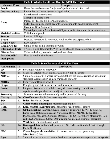
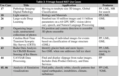
Tables 1 to 3 summarize characteristics of the 51 use cases, which we will combine with other input for the Ogres. Note that Big Data and parallel programming are intrinsically linked as any Big Data analysis is inevitably processed in parallel. Parallel computing is almost always implemented by dividing the data between processors (data decomposition); the richness here is illustrated in Table 1 which lists the members of space that is decomposed for different use cases; of course these sources of parallelism are broadly applicable outside the 51 use cases they were extracted from. In Table 2, we identify 15 use case features that will be used later as components of the Ogre facets. The second column of Table 2 lists our estimate of the number of use cases that illustrate this feature; note these are not exclusive so any one use case will illustrate many features.
It’s important to note that machine learning is commonly used but there is an interesting distinction between what are termed Local (LML) and Global machine learning (GML) in Table 2. In LML, there is parallelism over items of Table 1 and machine learning is applied separately to each item; needed machine learning parallelism is limited and is typified by use of accelerators (GPU). In GML, the machine learning is applied over the full dataset with MapReduce, MPI or equivalent. Typically GML comes from maximum likelihood or χ2 with a sum over the data items – documents, sequences, items to
squares and is illustrated by algorithms like PageRank, clustering/community detection, mixture models, topic determination, Multidimensional scaling, and (Deep) Learning Networks. Somewhat quixotically, GML can be termed Exascale Global Optimization or EGO.
Table 1: What is Parallelism Over for NIST Use Cases?
General Class Examples
People Users (but see below) or Subjects of application and often both
Decision makers Researchers or doctors (users of application)
Items
Experimental observations Contents of online store
Images or “Electronic Information nuggets”
EMR: Electronic Medical Records (often similar to people parallelism) Protein or Gene Sequences
Material properties, Manufactured Object specifications, etc., in custom dataset
Modelled entities Vehicles and people
Sensors Internet of Things
Events Detected anomalies in telescope, credit card or atmospheric data
Graph Nodes RDF databases
Regular Nodes Simple nodes as in a learning network
Information Units Tweets, Blogs, Documents, Web Pages, etc. and characters/words in them
Files or data To be backed up, moved or assigned metadata
Particles/cells/ mesh points
Used in parallel simulations
Table 2: Some Features of NIST Use Cases
Abbreviation # Description
PP 26 Pleasingly Parallel or Map Only
MR 18 Classic MapReduce MR (add MRStat below for full count)
MRStat 7 Simple version of MR where key computations are simple reduction as found in statistical averages such as histograms and averages
MRIter 23 Iterative MapReduce or MPI
Graph 9 Complex graph data structure needed in analysis
Fusion 11 Integrate diverse data to aid discovery/decision making; could involve sophisticated algorithms or could just be a portal
Streaming 41 Some data comes in incrementally and is processed this way
Classify 30 Classification: divide data into categories
S/Q 12 Index, Search and Query
CF 4 Collaborative Filtering for recommender engines
LML 36 Local Machine Learning (Independent for each parallel entity)
GML 23 Global Machine Learning: Deep Learning, Clustering, LDA, PLSI, MDS, Large Scale Optimizations as in Variational Bayes, MCMC, Lifted Belief Propagation, Stochastic Gradient Descent, L-BFGS, Levenberg-Marquardt . Can call EGO or Exascale Global Optimization with scalable parallel algorithm 51 Workflow: Universal so no label
GIS 16 Geotagged data and often displayed in ESRI, Microsoft Virtual Earth, Google Earth, GeoServer etc.
HPC 5 Classic large-scale simulation of cosmos, materials, etc. generating (visualization) data
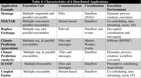
The difference between LML and GML is illustrated in Table 3, which contrasts 9 of the 51 NIST use cases that involve image based data. For example, use case 18 with light source data is largely
independent machine learning on each image from the source i.e. LML. In contrast deep learning in use case 26, is constructing a learning network integrating all the images.
2.4 Properties of distributed use cases
In the process of reduction and classification, the authors of [2, 3] analyze the structure of applications and find commonalities; they introduce the term “vectors” to capture four essentially orthogonal but critical properties that determine both the development and the execution of the application. These vectors are: execution unit, communication, coordination and an execution environment. The first three are internal properties of a distributed application, whereas the latter is essentially an external property. Based upon recurring values of vectors the authors propose a set of common patterns that help elucidate the structure of the distributed applications. It is worth noting, that vectors and patterns for distributed applications do not provide insight into performance aspects of the applications.
[image:5.612.69.538.135.433.2]In [2], the authors propose a framework for describing applications, distributed and dynamic data and infrastructure. Figure 1 shows the data lifecycle model used for the analysis capturing both applications using sensor and computationally generated data.
[image:5.612.74.540.623.673.2]Figure 1 Application Stages Table 3: 9 Image-based NIST Use Cases
Use Case Title Application Features
17 Pathology Imaging/ Digital Pathology
Moving to terabyte size 3D images, Global Classification
PP, LML, MR for search
18 Light sources Biology and Materials PP, LML
26 Large-scale Deep Learning
Stanford ran 10 million images and 11 billion parameters on a 64 GPU HPC; vision (drive car), speech, and Natural Language Processing
GML
27 Organizing large-scale, unstructured collections of photos
Fit position and camera direction to assemble 3D photo ensemble
GML
36 Catalina Real-Time Transient Synoptic Sky Survey (CRTS)
Processing of individual images for events based on classification of image structure (GML)
PP, LML, GML
43 Radar Data Analysis for CReSIS Remote Sensing of Ice Sheets
Identify glacier beds and snow layers See GML when one addresses full ice sheet
PP, LML moving to GML
44 UAVSAR Data
Processing,
Find and display slippage from radar images. Includes Data Product Delivery, and Data Services
PP
45, 46 Analysis of Simulation visualizations
Find paths, classify orbits, classify patterns that signal earthquakes, instabilities, climate, turbulence
The authors call out the Big Data aspects, the dynamic aspects and the distributed aspects of a large set of applications, and introduce quantitative estimates for various performance related properties.
The Table 4 below (from [3]) shows the specific values of the “DPA vectors” for the set of six distinct applications investigated. It is interesting to note that the categorization did not lead to well-defined and non-overlapping classification of application, as the complexity of considering the end-to-end aspects and the diverse ways in which applications are utilized, resulted in classes that had overlapping
characteristics.
3. The Big Data Ogres and their Three Facets
Synthesizing lessons learned from HPC, distributed applications and the NIST use case, given
above we argue that there is a need to construct classes of
mini-applications that facilitate the understanding and
characterization of the Big Data properties of these
applications.
We further introduce 3 facets or classification dimensions or features to categorize Big Data applications. These are Problem architecture, Computational features and Data Source or Style. There are of course other ways of looking at the Ogres and our work should be treated as an initial suggestion for further discussion. These facets build on earlier discussion – especially Table 2. Note that a given application can be made up ofcomponents with different characteristics in Ogre Facet classification. We will reference the 7
computational giants G1-G7 from the NRC report [8] recorded in Table 5. These are important big data patterns but the Ogres go into more detail. The final subsection discusses a selection of kernel Ogres focusing on analytics. We intend to follow up with other Ogre “mini-apps” or “kernels” covering areas like data intensive workflows.
[image:6.612.69.535.185.444.2]3.1 Problem Architecture Facet of Ogres
Table 4: Characteristics of 6 Distributed Applications Application
Example
Execution Unit Communication Coordination Execution Environment Montage Multiple sequential and
parallel executable
Files Dataflow
(DAG)
Dynamic process creation, execution
NEKTAR Multiple concurrent parallel executables
Stream based Dataflow Co-scheduling, data streaming, async. I/O
Replica-Exchange
Multiple seq. and parallel executables
Pub/sub Dataflow and
events Decoupled coordination and messaging Climate Prediction (generation)
Multiple seq. & parallel executables Files and messages Master-Worker, events @Home (BOINC) Climate Prediction (analysis)
Multiple seq. & parallel executables
Files and messages
Dataflow Dynamics process creation, workflow execution
SCOOP Multiple Executable Files and messages
Dataflow Preemptive scheduling, reservations
Coupled Fusion
Multiple executable Stream-based Dataflow Co-scheduling, data streaming, async I/O
Table 5: 7 Computational Giants of Massive Data Analysis [8] G1 Basic Statistics
G2 Generalized N-Body Problems
G3 Graph-Theoretic Computations
G4 Linear Algebraic Computations
G5 Optimizations
G6 Integration
This facet describes the overall structure of the application and determines the overall software and is an important driver of the software and hardware architecture discussed later. We have already stressed the importance of and distinction between Local (LML) and Global (GML) Machine Learning. These are often associated with Expectation Maximization and Steepest descent methods.
3.2 Computational features Facet of Ogres
Table 7: Computational Features Facet of Ogres Flops per byte: important for performance
Communication Interconnect requirements; Is application (graph) constant or dynamic?
Most applications consist of a set of interconnected entities; is this regular as a set of pixels or is it a complicated irregular graph?
Is communication BSP or Asynchronous? In latter case shared memory may be attractive; Are algorithms Iterative or not?
Data Abstraction: key-value, pixel, graph, vector, HDF5 etc. Are data points in metric or non-metric spaces (G2)?
Is algorithm O(N2) or O(N) (up to logs) for N points per iteration (G2)
Core libraries needed: matrix-matrix/vector algebra, conjugate gradient, reduction, broadcast …. (G4) This facet contains application characteristics that are familiar from the simulation domain. Distinctive are the important data abstraction layer that we would recommend highlighting in the software
architecture rather than burying as now in particular packages like Hadoop (key-value) and Giraph (graph). Simulations are often setup in well-defined physical spaces but data is often more abstract and the algorithms are typically quite different for metric and non-metric spaces. In contrast to the problem architecture facet, the computational features facet have a direct handle/relevance to performance. Note non-metric space algorithms are often O(N2). As discussed in the NRC report, there is a lot of opportunity
to incorporate sophisticated new algorithms to reduce O(N2) to O(N and logs). This is commonly used in
search and sort algorithms but not yet in computation in spite of promising initial work [8, 18, 19]
3.3 Data Source and Data Style Facet of Ogres
Table 8: Data Source and Style Facet of Ogres
SQL or NoSQL: NoSQL includes Document, Column, Key-value, Graph, Triple store Other Enterprise data systems: 10 examples from NIST [1] integrate SQL/NoSQL
Set of Files: as managed in iRODS and extremely common in scientific research
File, Object, Block and Data-parallel (HDFS) raw storage: Separated from computing?
Internet of Things: 24 [20] to 50 (Cisco [21, 22]) billion devices on the Internet by 2020
Table 6: Problem Architecture Facet of Ogres (Meta or Macro Pattern) Pleasingly
Parallel
as in BLAST, Protein docking, some (bio-)imagery including Local Analytics or Local Machine Learning with pleasingly parallel filtering, as in light source data, radar images
Classic MapReduce
Search, Index and Query and Classification algorithms like collaborative filtering (G1 for MRStat in Table 2, G7)
GML Global Analytics or Global Machine Learning requiring iterative runtime (G5, G6)
Graph Problem set up as a graph as opposed to vector, grid (G3)
SPMD SPMD (Single Program Multiple Data)
BSP Bulk Synchronous Processing: well-defined compute-communication phases
Fusion or Workflow
Knowledge discovery often involves fusion of multiple methods. All applications often involve orchestration (workflow) of multiple components
Streaming: Incremental update of datasets with new algorithms to achieve real-time response (G7)
HPC simulations generate major (visualization) output that often needs to mined
GIS (Geographical Information Systems) provide attractive access to geospatial data Before data gets to compute system, there is often an initial data gathering phase which is characterized by a block size and timing. Block size varies from month (Remote Sensing, Seismic) today (genomic) to seconds or lower (Real time control, streaming)
There are storage/compute system styles: Shared, Dedicated, Permanent, Transient
Other characteristics are needed for permanent auxiliary/comparison datasets and these could be interdisciplinary, implying nontrivial data movement/replication
The facet of table 8 covers the acquisition, storage, management and access to the data. The mantra of bringing computing to the data is an important principle especially for the Internet of Things when it is often not practical as backend (clouds) needed to provide adequate computing. It is interesting that the HPC approach of large shared file systems using technologies like Lustre is rather different from
commercial systems that use databases or HDFS. Figure 1 stresses that an important source of data is the output of other programs as data is streamed through a workflow.
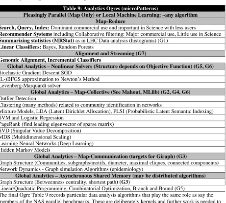
[image:8.612.75.536.292.707.2]3.4 Analytics Algorithm/Kernel Ogres
Table 9: Analytics Ogres (microPatterns)
Pleasingly Parallel (Map Only) or Local Machine Learning: ~any algorithm Map-Reduce
Search, Query, Index: Dominant commercial use and important in Science with less users
Recommender Systems including Collaborative filtering: Major commercial use, Little use in Science
Summarizing statistics (MRStat) as in LHC Data analysis (histograms) (G1)
Linear Classifiers: Bayes, Random Forests
Alignment and Streaming (G7) Genomic Alignment, Incremental Classifiers
Global Analytics – Nonlinear Solvers (Structure depends on Objective Function) (G5, G6)
Stochastic Gradient Descent SGD
(L-)BFGS approximation to Newton’s Method Levenberg-Marquardt solver
Global Analytics –Map-Collective (See Mahout, MLlib) (G2, G4, G6)
Outlier Detection
Clustering (many methods) related to community identification in networks
Mixture Models, LDA (Latent Dirichlet Allocation), PLSI (Probabilistic Latent Semantic Indexing) SVM and Logistic Regression
PageRank (find leading eigenvector of sparse matrix) SVD (Singular Value Decomposition)
MDS (Multidimensional Scaling)
Learning Neural Networks (Deep Learning) Hidden Markov Models
Global Analytics – Map-Communication (targets for Giraph) (G3)
Graph Structure (Communities, subgraphs/motifs, diameter, maximal cliques, connected components) Network Dynamics - Graph simulation Algorithms (epidemiology)
Global Analytics – Asynchronous Shared Memory (may be distributed algorithms)
Graph Structure (Betweenness centrality, shortest path) (G3)
Linear/Quadratic Programming, Combinatorial Optimization, Branch and Bound (G5)
specify more precisely. For example, there are many very different outlier and clustering algorithms corresponding to different scenarios (such as metric or non-metric spaces) and goals (such as tradeoff between performance and quality). We are developing with colleagues, benchmarks in the areas identified in Table 9. One should also introduce Ogres corresponding to full applications and workflows. These are important but not discussed here. We believe that the set of facets that will be needed to understand these other mini-apps will be common across Ogres.
4. Hardware and Software Architecture Issues
4.1 Five Important Architectures
Table 10: Distinctive Software/Hardware Architectures for Data Analytics 1 Pleasingly Parallel
(Map Only)
Includes local machine learning (LML) as in parallel decomposition over items and apply data processing to each item. Hadoop could be used but also other High Throughput Computing or Many task tools
2 Classic MapReduce Includes MRStat, search applications and those using collaborative filtering and motif finding implemented using classic MapReduce (Hadoop)
3 Iterative Map-Collective
Iterative MapReduce using Collective Communication as needed in clustering – Hadoop with Harp, Spark etc.
4 Iterative Map-Communication
Iterative MapReduce such as Giraph with point-to-point communication and includes most graph algorithms such as maximum clique, connected
component, finding diameter, community detection). Vary in difficulty of finding partitioning (classic parallel load balancing)
5 Shared (Large) Memory
Thread-based (event driven) graph algorithms such as shortest path and Betweenness centrality. Large memory applications
In table 10, we present 5 distinct problem architecture that map into 5 distinct system architectures which seem to cover the Ogres and their facets discussed in previous section. 10.5 is the shared memory
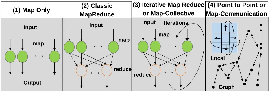
[image:9.612.71.538.498.658.2]architecture needed for some graph algorithms that perform better here and also for some large memory applications. The central architectures are 10.1 to 10.4 which correspond exactly to the four forms of MapReduce that we have presented previously [23] but are summarized in figure 2. Note this only describes some core features of the facets in tables 6 and 7. There are many other issues that need to be addressed including support of workflow and the data systems captured in the facets of table 8.
Figure 2: The Four forms of MapReduce that correspond to the four architectures of Table 10.1-10.4 Note that we separate Map-Collective [24, 25] and Map-(Point to Point) Communication following the Apache projects Hadoop, Spark and Giraph that focus on these cases. These programming models or run
(1) Map Only
(4) Point to Point or
Map-Communication (3) Iterative Map Reduce
or Map-Collective (2) Classic
MapReduce
Input
map
reduce
Input
map
reduce
Iterations Input
Output map
Local
times differ in communication style, application abstraction (key-value versus graph) and possible scheduling/load-balancing. HPC with MPI suggests that one could integrate 10.3 and 10.4 into a single environment and this approach is illustrated by the Harp plug-in to Hadoop which supports both models.
4.2 Comparison between Data Intensive and Simulation Problems
We can use the Ogre facet analysis and the data analytics architectures to compare data intensive and simulation applications. There are some clear similarities with looking back at table 6, “Pleasingly parallel” (10.1), BSP and SPMD common in both arenas. However the Classic MapReduce architecture (10.2) is a major big data paradigm but much less common in simulations with one example between the execution of multiple simulations (as in Quantum Monte Carlo) followed by a reduce operation to collect the results of different simulations. The Iterative Map-Collective architecture (10.3) is common in much Big Data analytics as in clustering where there is no local graph structure and the parallel algorithms involve large scale collectives but no point to point communication. The same structure is seen in N-body (long range force) or other “all-pairs” simulations without the locality typical from discretizing
differential operators.
Many simulation problems have the Map-Communication (10.4) architecture with many smallish point-to-point messages coming from local interactions between points defining system to be simulated. The importance of sparse data structures and algorithms is well understood in simulations and is seen in some Big Data problems such as PageRank, which calculates the leading eigenvector of the sparse matrix formed by internet site links. Other Big Data sparse data structures are seen in user-item ratings and bags of words problem. Most items are rated by few users and many documents contain a small fraction of the word vocabulary. However important data analytics involve full matrix algorithms and for example recent papers [26, 27] on a new Multi-Dimensional Scaling method use conjugate gradient solvers with full matrices as opposed to the new sparse conjugate gradient benchmark HPCG being developed for supercomputer (Top500) evaluations [28].
Note that there are similarities between some Big Data graph problems and particle simulations with an unusual potential defined by the graph node connectivity. Both use the Map-Communication architecture and the links in a Big Data graph are equivalent to strength of force between the graph nodes considered as particles. In this analogy, many Big Data problems are “long range force” corresponding to a graph where all nodes are linked to each other. As in simulation case, these O(N2) problems are typically very
compute intense but straightforward to parallelize efficiently. It is interesting to consider the analogue of the “fast multipole” methods for the fully connected Big Data problems which can dramatically improve the performance to O(N) or O(NlogN) as discussed in Sec. 3.3. Finally note the network connections used in deep learning are sparse but in recent image interpretation studies [29], the network weights are block sparse (corresponding to links to pixel blocks) and can be formulated as full matrix operations with GPUs and MPI running efficiently with these blocks.
The final architecture 10.5 (Shared Memory) is important in some applications but not heavily used in either simulations or Big Data although large memory systems are used extensively in gene assembly applications.
The above discussion focuses on a qualitative comparison of Big Data applications with traditional simulation (HPC) applications viz., comparing the structure. As can be seen there are similarities as well as points of distinction. It is likely however, that that there will be significant differences in the
ratios (e.g., ratio of computing to I/O, ratio of memory to I/O etc.) characterizing the computational feature will be different. We will investigate both quantitative and qualitative differences in future work.
4.3 A Big Data Software Environment
Table11: Kaleidoscope of (Apache) Big Data Stack (ABDS) and HPC Technologies
Cross-Cutting
Functionalities
Message Protocols:Thrift, Protobuf
Distributed Coordination:
Zookeeper, JGroups
Security & Privacy:
InCommon, OpenStack Keystone, LDAP
Monitoring:
Ambari, Ganglia, Nagios, Inca
Workflow-Orchestration: Oozie, ODE, Airavata, OODT (Tools), Pegasus, Kepler, Swift, Taverna, Trident, ActiveBPEL, BioKepler, Galaxy, IPython
Application and Analytics: Mahout , MLlib , MLbase, CompLearn, R, Bioconductor, ImageJ, Scalapack, PetSc
High level Programming: Hive, HCatalog, Pig, Shark, MRQL, Impala, Sawzall, Drill
Basic Programming model and runtime, SPMD, Streaming, MapReduce, MPI: Hadoop, Spark, Twister, Stratosphere, Tez, Hama, Storm, S4, Samza, Giraph, Pregel, Pegasus
Inter process communication Collectives, point-to-point, publish-subscribe:
Hadoop, Spark, Harp, MPI, Netty, ZeroMQ, ActiveMQ, QPid, Kafka, Kestrel
In-memory databases/caches: GORA (general object from NoSQL), Memcached, Redis (key value), Hazelcast, Ehcache
Object-relational mapping: Hibernate, OpenJPA and JDBC Standard
Extraction Tools: UIMA, Tika
SQL: Oracle, MySQL, Phoenix, SciDB
NoSQL: HBase, Accumulo, Cassandra, Solandra, MongoDB, CouchDB, Lucene, Solr, Berkeley DB, Azure Table, Dynamo, Riak, Voldemort. Neo4J, Yarcdata, Jena, Sesame, AllegroGraph, RYA
File management: iRODS
Data Transport: BitTorrent, HTTP, FTP, SSH, Globus Online (GridFTP)
Cluster Resource Management: Mesos, Yarn, Helix, Llama, Condor, SGE, OpenPBS, Moab, Slurm, Torque
File systems: Swift, Cinder, Ceph, FUSE, Gluster, Lustre, GPFS, GFFS
Interoperability: Whirr, JClouds, OCCI, CDMI
DevOps: Docker, Puppet, Chef, Ansible, Boto, Libcloud, Cobbler, CloudMesh
IaaS Management from HPC to hypervisors: OpenStack, OpenNebula, Eucalyptus, CloudStack, vCloud, Amazon, Azure, Google
We have described elsewhere [30-32] how we propose to implement Big Data applications exploiting the HPBDS architecture sketched in Table 11 [33]. This combines the best practice commercial Big Data software with an emphasis on Apache projects with HPC subsystems. Table 11 illustrates by green shading those layers where HPC adds significant value to the Apache stack ABDS. Note that high performance communication is known to be critical for simulations but it is also essential for many science big data applications. Commercial applications have large “search” (10.2) components
corresponding to the huge number of users accessing commercial Big Data systems. In science, this step is necessary – especially for good data management – but is a much lower fraction of system use as the number of scientists accessing data is much lower than number of users of commercial Big Data.
5 Discussion and Conclusion
that are generally considered to be of relevance/importance to science and engineering using a context that includes a limited set of commercial problems. Using this broad range of Big Data applications as our working set, this paper is an attempt at distilling the Big Data properties (facets) and organizing the plethora of disparate Big Data applications using these properties. Although we validate using analytics kernels, this classification / organization will in turn shed light on and help provide better understanding of both the structure of S&E Big Data applications, as well as determinants of their performance. In Section 4, we show how a deeper appreciation of the Ogre facets will help design and implement better hardware and software systems.
Appendix 71 NIST Use Cases
The 71 NIST Use Cases with number in each broad area
Government Operation(4): National Archives and Records Administration, Census Bureau
Commercial(8): Finance in Cloud, Cloud Backup, Mendeley (Citations), Netflix, Web Search, Digital Materials, Cargo shipping (as in UPS)
Defense(3): Sensors, Image surveillance, Situation Assessment
Healthcare and Life Sciences(10): Medical records, Graph and Probabilistic analysis, Pathology, Bioimaging, Genomics, Epidemiology, People Activity models, Biodiversity
Deep Learning and Social Media(6): Driving Car, Geolocate images/cameras, Twitter, Crowd Sourcing, Network Science, NIST benchmark datasets
The Ecosystem for Research(4): Metadata, Collaboration, Language Translation, Light source experiments
Astronomy and Physics(5): Sky Surveys including comparison to simulation, Large Hadron Collider at CERN, Belle Accelerator II in Japan
Earth, Environmental and Polar Science(10): Radar Scattering in Atmosphere, Earthquake, Ocean, Earth Observation, Ice sheet Radar scattering, Earth radar mapping, Climate simulation datasets, Atmospheric turbulence identification, Subsurface Biogeochemistry (microbes to watersheds), AmeriFlux and FLUXNET gas sensors
Energy(1): Smart grid
Enterprise Data Systems(10): Multiple users performing interactive queries and updates on a database with basic availability and eventual consistency (BASE); Perform real time analytics on data source streams and notify users when specified events occur; Move data from external data sources into a highly horizontally scalable data store, transform it using highly horizontally scalable processing (e.g. Map-Reduce), and return it to the horizontally scalable data store (ELT); Perform batch analytics on the data in a highly horizontally scalable data store using highly horizontally scalable processing (e.g MapReduce) with a user-friendly interface (e.g. SQL like); Perform interactive analytics on data in analytics-optimized database; Visualize data extracted from horizontally scalable Big Data store; Move data from a highly horizontally scalable data store into a traditional Enterprise Data Warehouse; Extract, process, and move data from data stores to archives; Combine data from Cloud databases and on premise data stores for analytics, data mining, and/or machine learning; Orchestrate multiple sequential and parallel data transformations and/or analytic processing using a workflow manager
Security & Privacy(10): Consumer Digital Media Usage; Nielsen Homescan; Web Traffic Analytics; Health Information Exchange; Personal Genetic Privacy; Pharma Clinic Trial Data Sharing; Cyber-security; Aviation Industry; Military - Unmanned Vehicle sensor data; Education - “Common Core” Student Performance Reporting
References
1. NIST. Big Data Initiative Reports from V1. 2013 [accessed 2014 March 26]; Report at
2. Shantenu Jha, Neil Chue Hong, Simon Dobson, Daniel S. Katz, Andre Luckow, Omer Rana, and Yogesh Simmhan, Introducing Distributed Dynamic Data-intensive (D3) Science: Understanding Applications and Infrastructure. 2014. https://dl.dropboxusercontent.com/u/52814242/3dpas-draft.v0.1.pdf.
3. S. Jha, M. Cole, D. Katz, O. Rana, M. Parashar, and J. Weissman, Distributed Computing Practice for Large-Scale Science & Engineering Applications. Concurrency and Computation: Practice and Experience, 2013. 25(11): p. 1559-1585. DOI:http://dx.doi.org/10.1002/cpe.2897
4. R open source statistical library. [accessed 2012 December 8]; Available from: http://www.r-project.org/. 5. Apache Mahout Scalable machine learning and data mining [accessed 2012 August 22]; Available from:
http://mahout.apache.org/.
6. Machine Learning Library (MLlib). [accessed 2014 April 1]; Available from:
http://spark.apache.org/docs/0.9.0/mllib-guide.html.
7. NIST, NIST Big Data Public Working Group (NBD-PWG) Use Cases and Requirements. 2013.
http://bigdatawg.nist.gov/usecases.php
8. Committee on the Analysis of Massive Data, Committee on Applied and Theoretical Statistics, Board on Mathematical Sciences and Their Applications, and Division on Engineering and Physical Sciences,
Frontiers in Massive Data Analysis. 2013: The National Academies Press,.
http://www.nap.edu/catalog.php?record_id=18374
9. Berry, M., D. Chen, P. Koss, D. Kuck, S. Lo, Y. Pang, L. Pointer, R. Roloff, A. Sameh, E. Clementi, S. Chin, D. Schneider, G. Fox, P. Messina, D. Walker, C. Hsiung, J. Schwarzmeier, K. Lue, S. Orszag, F. Seidl, O. Johnson, R. Goodrum, and J. Martin, The Perfect Club Benchmarks: Effective Performance Evaluation of Supercomputers. International Journal of High Performance Computing Applications, September 1, 1989, 1989. 3(3): p. 5-40. DOI:10.1177/109434208900300302.
http://hpc.sagepub.com/content/3/3/5.abstract
10. NASA Advanced Supercomputing Division. NAS Parallel Benchmarks. 1991 [accessed 2014 March 28]; Available from: https://www.nas.nasa.gov/publications/npb.html.
11. Rob F. Van der Wijngaart, Srinivas Sridharan, and Victor W. Lee, Extending the BT NAS parallel benchmark to exascale computing, in Proceedings of the International Conference on High Performance Computing, Networking, Storage and Analysis. 2012, IEEE Computer Society Press. Salt Lake City, Utah. pages. 1-9.
12. PARKBENCH (PARallel Kernels and BENCHmarks). 1996 [accessed 2014 July 19]; Available from:
http://www.netlib.org/parkbench/.
13. Jack Dongarra, Erich Strohmaier, and Michael Resch. Top 500 Supercomputer Sites. 2014 [accessed 2014 July 19]; Available from: http://www.top500.org/.
14. A. Petitet, R. C. Whaley, J. Dongarra, and A. Cleary. HPL - A Portable Implementation of the High-Performance Linpack Benchmark for Distributed-Memory Computers. 2008 September 10 [accessed 2014 July 19,]; Available from: http://www.netlib.org/benchmark/hpl/.
15. R. Barrett, M. Berry, T. F. Chan, J. Demmel, J. Donato, J. Dongarra, V. Eijkhout, R. Pozo, C. Romine, and H. Van der Vorst, Templates for the Solution of Linear Systems: Building Blocks for Iterative Methods, 2nd Edition. 1994, Philadelphia, PA: SIAM. http://www.netlib.org/linalg/html_templates/Templates.html
16. Timothy G. Mattson, Beverly A. Sanders, and Berna L. Massingill, Patterns for Parallel Programming. 2013: Addison-Wesley Professional. ISBN:0321940784
17. Asanovic, K., R. Bodik, B.C. Catanzaro, J.J. Gebis, P. Husbands, K. Keutzer, D.A. Patterson, W.L. Plishker, J. Shalf, S.W. Williams, and K.A. Yelick. The Landscape of Parallel Computing Research: A View from Berkeley. 2006 December 18 [accessed 2009 December]; Available from:
http://www.eecs.berkeley.edu/Pubs/TechRpts/2006/EECS-2006-183.html.
18. P. Ram, D. Lee, W. March, and A.G. Gray. Linear-time algorithms for pairwise statistical problems. in
Advances in Neural Information Processing Systems. NIPS 2009. Vancouver, BC.
19. Judy Qiu, Jaliya Ekanayake, Thilina Gunarathne, Jong Youl Choi, Seung-Hee Bae, Yang Ruan, Saliya Ekanayake, Stephen Wu, Scott Beason, Geoffrey Fox, Mina Rho, and Haixu Tang, Data Intensive Computing for Bioinformatics, Chapter in Data Intensive Distributed Computing, Tevik Kosar, Editor. 2011, IGI Publishers.
http://grids.ucs.indiana.edu/ptliupages/publications/DataIntensiveComputing_BookChapter.pdf.
21. Cisco. Visual Networking Index: Forecast and Methodology, 2012–2017. 2013 May 29 [accessed 2013 August 14]; Available from:
http://www.cisco.com/en/US/solutions/collateral/ns341/ns525/ns537/ns705/ns827/white_paper_c11-481360_ns827_Networking_Solutions_White_Paper.html.
22. Cisco Internet Business Solutions Group (IBSG) (Dave Evans). The Internet of Things: How the Next Evolution of the Internet Is Changing Everything. 2011 April [accessed 2013 August 14]; Available from:
http://www.cisco.com/web/about/ac79/docs/innov/IoT_IBSG_0411FINAL.pdf.
23. Jaliya Ekanayake, Thilina Gunarathne, Judy Qiu, Geoffrey Fox, Scott Beason, Jong Youl Choi, Yang Ruan, Seung-Hee Bae, and Hui Li, Applicability of DryadLINQ to Scientific Applications. January 30, 2010, Community Grids Laboratory, Indiana University.
http://grids.ucs.indiana.edu/ptliupages/publications/DryadReport.pdf.
24. J.Ekanayake, H.Li, B.Zhang, T.Gunarathne, S.Bae, J.Qiu, and G.Fox, Twister: A Runtime for iterative MapReduce, in Proceedings of the First International Workshop on MapReduce and its Applications of ACM HPDC 2010 conference June 20-25, 2010. 2010, ACM. Chicago, Illinois.
http://grids.ucs.indiana.edu/ptliupages/publications/hpdc-camera-ready-submission.pdf.
25. Bingjing Zhang, Yang Ruan, Tak-Lon Wu, Judy Qiu, Adam Hughes, and Geoffrey Fox, Applying Twister to Scientific Applications, in CloudCom 2010. November 30-December 3, 2010. IUPUI Conference Center Indianapolis. http://grids.ucs.indiana.edu/ptliupages/publications/PID1510523.pdf.
26. Yang Ruan and Geoffrey Fox, A Robust and Scalable Solution for Interpolative Multidimensional Scaling with Weighting, in 9th International conference on e-Science. October 22-25, 2013. Beijing. DOI:
http://dx.doi.org/10.1109/eScience.2013.30.
27. Yang Ruan, Geoffrey L. House, Saliya Ekanayake, Ursel Schütte, James D. Bever, Haixu Tang, and Geoffrey Fox, Integration of Clustering and Multidimensional Scaling to Determine Phylogenetic Trees as Spherical Phylograms Visualized in 3 Dimensions, in FIRST INTERNATIONAL WORKSHOP ON CLOUD FOR BIO (C4Bio 2014). May 26-29, 2014. IEEE/ACM CCGrid 2014 Chicago. pages. 26-29.
http://grids.ucs.indiana.edu/ptliupages/publications/PhylogeneticTreeDisplayWithClustering.pdf. 28. Jack Dongarra and Michael A. Heroux. Toward a New Metric for Ranking High Performance Computing
Systems. 2013 June [accessed 2014 July 19,]; SANDIA REPORT SAND2013-4744 (Defines HPCG) Available from: http://www.sandia.gov/~maherou/docs/HPCG-Benchmark.pdf.
29. Adam Coates, Brody Huval, Tao Wang, David Wu, Bryan Catanzaro, and Andrew Ng. Deep learning with COTS HPC systems. in Proceedings of the 30th International Conference on Machine Learning (ICML-13)
2013.
30. Wo Chang. ISO/IEC JTC 1 Study Group on Big Data in 1st Big Data Interoperability Framework Workshop: Building Robust Big Data Ecosystem. March 18-21 2014. SDSC, San Diego CA: NIST. 31. Geoffrey Fox, Judy Qiu, and Shantenu Jha, High Performance High Functionality Big Data Software
Stack, in Big Data and Extreme-scale Computing (BDEC). 2014. Fukuoka, Japan.
http://www.exascale.org/bdec/sites/www.exascale.org.bdec/files/whitepapers/fox.pdf.
32. Shantenu Jha, Judy Qiu, Andre Luckow, Pradeep Mantha, and Geoffrey C. Fox, A Tale of Two Data-Intensive Approaches: Applications, Architectures and Infrastructure, in 3rd International IEEE Congress on Big Data Application and Experience Track. June 27- July 2, 2014. Anchorage, Alaska.
http://arxiv.org/abs/1403.1528.