Abstract: Financial Time series analysis (FTSA) is concerned with theory and practice of asset valuation over time. Generally, FTSA is useful for forecasting the asset volatility. This paper proposes the discrete S-Transform technique driven by Gaussian kernel for the estimation of volatility in FTSA. S-Transform is found to be a better tool in finding the time frequency resolution so as to predict and estimate the risk and returns of financial market. S-Transform prediction on two different bench mark data sets namely, Standard & Poor(S&P) 500 and Dow Jones Industrial Average(DJIA) index clearly indicates its superiority for the prediction of short and long-term trends in stock markets.
Key words: Volatility, S-Transform, Gaussia kernel
I. INTRODUCTION
Among the various works in Mathematical Finance Theory and practice of asset value discrete time models, continuous time models of financial markets and a handful of models of interest rates provide a substantial substratum for stock market pricing, leading to judicious and timely inferences. In stochastic analysis of financial time series, modeling of volatility is a vital topic. Four aspects – namely, price dynamics, trading strategies, viable and complete financial markets and bond price dynamics play a dominant role in this model [1]. Financial analysts without a single exception carry out various kinds of research to beat a stock market, in order to obtain consistently higher return rates than average return of a market, always keeping the market risks in focus. One of the parameters of the performance of any mutual fund is a sizable return to an investment. If Pt is the price of an asset at time index t and Rt is the one-period simple net return, then
1 1
t t t t
P
P
P
R
--- (1) and cumulative returns of k periods financial time series is calculated using the formula [2],1 + pt (k) = (1+R1)(1+R2)….(1+Rk) =
k
t
t
R
1
)
1
(
---(2)There are two glaring traditional techniques of a financial time series – (i) problems related to machine learning methods [3-7], including stochastic methods and (ii) econometric method which deals a statistical model based on a set of parameters. The underlying assumption of these models is that logarithm of the prices follows normal
Revised Manuscript Received on September 06, 2019
Dr.R.Seethalakshmi, APIII, School of Arts, Science & Humanities, SASTRA Deemed University, Thanjavur, India.
Rahul R., Student, School of Computing, SASTRA Deemed University, Thanjavur, India.
Dr.Vijayabanu C, Associate Professor, School of Management, SASTRA Deemed University, Thanjavur, India.
distribution which is rather subjective. A problem related to statistical methods is that price movements cannot be modelled on single probability density function. Added to it, for various time windows, different patterns cannot be described by one stationary model. It has broadly been approved in principle that no single method can be employed for exact prediction of volatility. Due to the fact that market rate follows random walk, no significant predictability has been ensured so far and these models generally face harsh challenges both theoretically and empirically.
A. Definition, Meaning and Importance
Generally, Volatility is defined to be the relative rate in which the price of a security increases or decreases. Volatility is usually found by calculating the annualized standard deviation of daily change in price. When the rapid change in price of a stock takes place over short periods of time, it is said to have high volatility. If the price hardly changes, it has low volatility. The importance of volatility in option trading depends on market prices that change from one instant to the next. Usually, increased volatility is associated with falling stock prices. In general, jumps in volatility keep up a correspondence to a declining stock price. But rapid increasing markets also have a higher level of volatility. Periods of higher volatility are often caused by an emotional driven market.
B. Fundamental Assumptions
A variety of statistical models predicting the returns are reported in the reference [8,10,11,12]. Most of such statistical methods work under the main assumption that the population distribution is Gaussian for stock markets or binomial for bonds and debt market [9]. Returns to follow normal distribution and underlying prices to follow lognormal distributions are the fundamental assumptions used in assets models. Hence, in the distribution of returns, volatility is the deviation of returns from the mean and 10% yearly Volatility represents that in one year the returns will be within c - 10%, c +10% with 68.3% probability, where c is the mean of the distribution.
C. Methods of Measuring Volatility
Historical volatility also termed as realized volatility, is the price movements of assets in the past, while implied
volatility refers to determining the market outlook of the asset's future volatility. Studying changes in the historical volatility of an asset can facilitate recognizing a normal volatility range, deviations from it, and subsequent trading opportunities.
S-Transform Based Analysis for Stock Market
Volatility Estimation
The two kinds of historical volatility namely statistical volatility, High Low Range Volatility or Parkinson's historical volatility use various statistical measures such as standard deviation, simple moving average, exponentially weighted moving average. The other kinds of volatility that include the volatility index and intraday volatility are more about the sensitivity of time localized market variations.
D. Time Series Data Analysis and Related Software
Charting the historical information of time series data of stock market through implied and realized volatility, statistical measurements such as correlation and Beta, Skew and Kurtosis are found to be useful for determining interrelation between different indicators visually, and historical end-of-day data is used to perform technical analysis. General methods of time series data analysis include Box-Jenkins ARIMA models, Multivariate models and Holt-Winters Exponential Smoothing models. However, the evolution of statistical learning theory in the context of the advent of computer science paved a broader way to accommodate all these models for constructing several machine learning techniques such as neural networks, support vector machines, genetic algorithm, Hidden Markov models or some of their combinatorial structures as hybrid ones to serve as online indicators of stock markets[13].
E. Nonlinearity in The Financial Time Series Data and
Volatility Concept
There are various traditional forms of statistical models to predict volatile financial time series [14]. Sometimes high stock movement was observed without any apparent news. The time bound data exhibit the irrational price movement, whose part of a pattern is usually called noise. Another inherent problem of statistical methods is that price movements cannot be modelled on one single probability density function(pdf) [15]. Some of the multivariate time series problems are addressed by prediction functions which can map the inputs with the desired output from the different database, which cause an additional noise term that stems from the parameters of the underlying distributions. Examples include the regression of stock market volatility from word counts in consecutive financial news articles [16,17] and the categorization of consecutive news articles [18,19]. So, the nonlinearity in the financial data is accounted for by four reasons. (i)Noisy data due to irrational price movement,(ii)Modeling impossibility through single pdf,(iii) Lack of best approximation function and (iv)Additional noise term from the parameters of statistical distributions. In order to address the nonlinearity in stock market data, Fast Fourier Transform (FFT) is found to be a useful tool that delivers real time pricing, while allowing for a realistic structure of asset returns that include extra kurtosis and stochastic volatility [20]Fourier transform of the entire time series contains information about the spectral components in a time series for a large class of practical applications. However, this information is inadequate. In these circumstances, FFT does not provide an exhaustive account in finance and a complete time frequency resolution of financial data leading to optimal solution which can forecast the future stock is scarcely seen in literature. Since more recently recorded data are to be given
slightly more weightage than historical data for finding better volatility estimates, in order to forecast the stock market, both features of financial data (in time and frequency domain) need be obtained for designing effective techniques to serve as online indicators of the stock market.
II. RELATED WORK
Various approaches followed by earlier researchers for forecasting the stock market status and other financial time series problems include: (i) Statistical approach, (ii) Mathematical modeling,(iii) Soft computing and (iv) transform approach. In statistical approach, researchers use statistical distributions to describe the data pattern and obtain the necessary parameters to characterize stock movements. However, determining these parameters was found to be a daunting task due to uncertainty in the data. Moreover, accounting for irrelevant data needs deeper insight into understanding the data pattern. Several works include statistical distributions such as normal, lognormal etc. [21-28]. The conditional variances involved in these models together with combination of lag length parameters characterize an interesting behaviour of asset prices which have an asymmetric effect on volatility called the leverage effect. However, these statistical estimations are not adequate in describing the frequency patterns of data which are necessary for better predictions and forecasting. In modelling approach, Markov models [29] provide probabilistic predictions which again necessitate closer values of earlier predictions, yet giving still approximate predictions. Moreover, this also does not provide long term predictions. Hence present-day researches work in Soft Computing approach [30], that is sensitive to market change and parameters of the data. This provides closer approximations due to the inherent ability of operators, training and testing phase while processing the data, removal of uncertainty in the earlier phase, to name a few. But transform approach provides a frequency based approach which talks about the large sized overlapped data in terms of samples and frequencies. The variants of S-transform [31] seem to provide reasonable resolution of samples and frequencies. Hence in this paper we have taken up S-transform for near future volatility predictions for processing moderate size data.
The Need for The Introduction of S-Transform
One such application that requires this type of relationship is forecast of stock market indices. Economic indicators [32] are the parameters that are directly or indirectly related to economy which has got close relationship with stock market indices. The three major attributes of economic indicators which are usually discussed in financial time series problems are: (i) relation to business cycle, (ii) frequency of the data and (iii) timings.
In timing, economic indicators can be leading, lagging or co-incidental. Stock market returns are „leading indicators‟ as they usually begin to decline before the decline of economy and improve well before the economy begins to come out of recession. Some economic indicators are immediately available and undergo change every minute, with the hidden frequency. Hence, in order to have both time and frequency representation of the stock market data which are non-stationary in nature, S-transform as discussed in section 4 is applied to different economic indicators to study various cycles involved in the business.
Continuous and Discrete S-Transform Tools and Their Applications
The S-transform, as proposed by Stockwell etal, 1996 [35], is a technique that localizes time frequency spectral component, which combines the individual advantages of STFT and CWT with a Gaussian window with width scales inversely and height varies linearly with the frequency. Moreover, S-transform can be considered as the phase correction of CWT. The mathematical expression of continuous S-transform is given by:
dt t if t f f t h f s
exp( 2 ( ))
2 ) ( exp 2 ) ( ) , ( 2 2 (3)
In the above equation, h is a continuous function of t, „f‟ is the frequency and
is a parameter that controls the position of the Gaussian window on t axis.Various versions of S – Transform used by the research community in different applications, their specific properties used in such applications and their relative merits and limitations are furnished in the Table 1.(Appendix) In our application of S-Transform, x(t) refers to closing value of the stock at a particular time t and f is a parameter that controls the location in the time line. The corresponding mother wavelet is defined by
w(t,f)= jft
f t
e
e
f
2 2 2 22
--- (4)
S-transform can also be expressed as Fourier spectrum X(f) of x(t).
(
)
exp
(
2
)
;
0
)
,
(
2 2 2f
d
e
f
f
X
f
S
i
(5) and Fourier spectrum can also be directly obtained from
)
,
(
f
S
by taking average of local spectra as X(f) =
f
d
S
(
,
)
(6)
and original stock value can be obtained by using Inverse S-transform
S f e d df
t
x( ) (
, ) 2 j f t
(7)
In this work, the recorded closing values of the market x(t) are all stored in the discrete form that can take the form x(k ,T), where T is the time sampling interval and k = 0,1, 2…. N-1 where N is the total sampling number.
From (4.3), it is observed that S-transform can be operated quickly by FT. Hence the discrete form of ST can be obtained by letting
Q
iT
,
and
f
n
/
NT
as0
)
,
(
2 2 1 0 2 2 2
n
e
e
NT
n
m
X
NT
n
iT
S
N i j k m n m N m (8)with
[
,
0
]
1
0
1 0
n
NT
m
x
N
iT
S
N m (9)where n,i , m takes the values from 0 , 1 , 2 , …., N – 1 and the discrete FT of x(kT) is expressed as
X
1 0 2)
(
1
N k N k n je
kT
x
N
NT
n
(10)Hence, by taking advantage of FFT, the discrete ST of x(t) can be computed in a fast manner. Clearly the output of S-transform is a k x n matrix, with hour corresponding to frequency and column pertaining to time. The S-transform amplitude matrix that is used to represent risk / return in the present study is obtained as
NT
n
kT
S
f
kT
A
,
,
(11)
The time frequency representation of the closing values of stock market data enables us to obtain base vectors in the frequency domain and the location vectors in time domain to construct the feature space and density estimates which can be shown in two dimensional and three-dimensional plots, which in turn reflect the information of the original data adequately. Moreover, finer scaling provides all data including the missed values, while frequencies provide the density, which together indicate the near future stock levels.
III. ALGORITHM, DATA AND METHODOLOGY
A. Stepwise Algorithm For Computation Of
Time-Frequency - Amplitude (Or) Time-Risk-Return Estimates Discrete S-Transform Algorithm
Step 1 : Get the time series data i.e., closing values verses time values.
Step 2 : Choose the appropriate sampling frequency (f) to determine number of risks (m).
Step 3 : Computation of Discrete Fourier Transform of X(kT) . With the help of the time series data and risk component (m) obtain the DCT for the given stock market data
1
,...,
2
,
1
,
0
)
(
1
1 0 2
N
n
e
kT
x
N
NT
n
X
N k N k n j (12)Step 4 : Calculation of S-Transform for initial distribution of stock market data
1 01
]
0
,
[
N mNT
m
x
N
iT
S
(13)Step 5 : Calculation of S-Transform for entire data sampled by step 2.
0
;
)
,
(
2 2 1 0 2 2 2
n
e
e
NT
n
m
X
NT
n
iT
S
N i j k m n m N m (14) Step 6 : Calculation of amplitude (Returns)A
NT
n
kT
S
f
kT
,
,
(15)Step 7 : Using the return, risk and time, obtain the three dimensional plot.
Step 8 : Change the sampling frequency (m) appropriately to obtain better estimates of risk / return.
The conventional methods of calculating volatility fail to consider the full range of observations. In fact, equal weights are being assigned in the formulas of our observations. Logically, the retrograde movement of the most recent data accounts more for forecasting the stock volatility then mere accumulation of „dated‟ data. It means recently collected
statistical data be reasonably given more weightage for forecasting purposes than the older data (For instance 52 years – 673 data as shown in below section .A model that deviates from this assumption is the weighted average moving exponentially.
B. Data : The Standard & Poor 500 data (S&P 500) for
discrete time modeling
[image:4.595.312.563.74.258.2]Discrete S-transform prediction system has been utilized for the prediction of real world financial time series data – S&P 500 data which is the weighted average of „500 leading companies‟ stock prices from their leading industrial sectors of the USA. The S&P 500 index is considered to be the benchmark indicator of the USA the health of its economy, reflecting the total market value of stock components at a particular period of time. Instead of 30 component stock prices in Dow Jones Industrial Average (DJIA), The S&P 500index provides the market value of 500 stocks. Though it includes stocks from different industries S&P 500 has some distinguishing characteristics such as sensitivity, predictability, scalability, to name a few. The technique mentioned in the introduction has been used to calculate the returns of the S&P 500 index. We have used the closing price index for future calculations. A sample of data obtained from [38] is shown in Table 2.
Table 2 A sample data of the experiment for the segment from July 6, 1998 to July 15, 1998
Date Open High Low Close Volu me Adj Close 06/07/ 1998 1146.4
2 1157.33
1145.0 3 1157. 33 1157. 33 5.15E+ 08 07/07/ 1998 1157.3
3 1159.81
1152.8 5 1154. 66 1154. 66 6.25E+ 08 08/07/ 1998 1154.6
6 1166.89
1154.6 6 1166. 38 1166. 38 6.07E+ 08 09/07/ 1998 1166.3
8 1166.38
1156.0 3 1158. 56 1158. 56 6.64E+ 08 10/07/ 1998 1158.5
7 1166.93
1150.8 8 1164. 33 1164. 33 5.76E+ 08 13/07/ 1998 1164.3
3 1166.98
1160.2 1 1165. 19 1165. 19 5.75E+ 08 14/07/ 1998 1165.1
9 1179.76
1165.1 9
1177. 58
1177.
58 7E+08 15/07/
1998
1177.5
8 1181.48
1174.7 3 1174. 81 1174. 81 7.24E+ 08
C. Volatility Estimation and Experimental Results
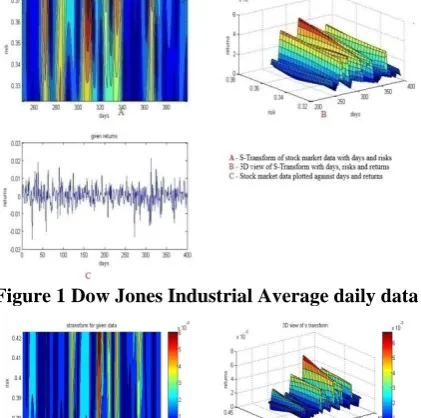
As explained in Section 1, stock market is a leading economic indicator. To carry out the analysis of business cycles, two different stock market data from the United States have been taken into account - one from DJIA and the other from S&P 500 index. From Jan 1952 to Jan 2006,673 data patterns representing the stock indices have been collected in a time series. Among these data, a set of 400 consecutive daily data have been processed to obtain intraday average and its S –transform simulations for risk-return representations are shown in figs(1) and (2). The corresponding S-transform based time and frequency resolution have also been shown.
Figure 1 Dow Jones Industrial Average daily data
[image:4.595.323.534.441.650.2]Similarly, the above mentioned 673 monthly data patterns have been processed to obtain monthly average and itsS transform simulations for risk return representations as shown in Fig. (3) and Fig (4), respectively. The time – frequency simulations have been shown in 2-D and 3-D plots.
[image:5.595.62.276.283.471.2]Figure 3 Dow Jones Industrial average monthly data
Figure 4 S&P 500 Monthly data
A sample data processed by S-transform algorithm generates amplitudes of the output in a matrix form exhibiting the return values. These results are displayed in Table 3.
Table 3A sample of volatility estimates for DJIA and S&P 500 data for the period of 1960 to 2011
Days Mean Varianc
e Days Mean Variance
54 2.45e-04 2.5e-03 310 0.00030
5 0.000497
55 2.53e-04 5.1e-03 311 0.00030
6 0.000995
56 2.52e-04 7.5e-03 312 0.00030
8 0.001492
57 2.53e-04 1.2e-03 313 0.00030
9 0.001989
58 2.51e-04 1.25e-03 314 0.00031
0 0.002486
Year Mean Varianc
e Year Mean Variance
2006 26.210 5.01 2004 217.33 3.69
2007 26.208 4.18 2005 217.31 8.15
2008 26.206 4.71 2006 217.29 2.33
2009 26.204 4.00 2007 217.28 1.63
2010 26.202 3.08 2008 217.26 3.56
From fig (3), we see that the maximum density estimates of data patterns using the Gaussian window kernel take place between 1950 to 2006. Similarly, simulations have been carried out for DJIA data and time frequency resolutions are shown in fig 4. The sideway movements of some of the data shown in fig 3(b) have got low density estimates from 1950 to 2006 as represented in fig 3(c). These low-density predictions are not accurate because of the unusual variations during the period which are usually classified as whipsaws (noisy).
A part of DJIA data, processed for obtaining mean and standard deviations (Volatility estimates)by earlier group of researchers [32] has also been processed by choosing n=5 ,N=400, m = 1 in Discrete S –Transform algorithm for calculating mean and by obtaining the frequency “f” for the calculation of standard deviation and found to be with good agreement with statistical calculation. To check for the continuation of local variation towards the risk / return, a lower sized DJIA & S&P 500 data have also been processed.
D. Prediction Performance
The prediction performance is evaluated by the statistical metrics namely the „Normalized Mean Squared Error‟ (NMSE) and „Mean Absolute Error‟(MAE) which are the deviation between actual and predicted values. For the DJIA data minimum and maximum NMSE are found to be 0.0786 and 1.345. Similarly, the minimum and maximum MAE are found to be 0.280 and 1.159.For other samples also, the experiments are repeated and the errors are found to be within these limits.In the same way, the performance of this transform is also evaluated among various samples of S&P500 data and the error has been observed to be well within the limits of (0.8, 1.42) for NMSE and (0.894, 1.192) for MAE. S-transform is capable of sensing both dense and lucid data for obtaining density estimates by using an appropriate kernel function such as Gaussian, bi-Gaussian and hyperbolic. It is observed that calculation of volatility estimate from S-transform expression is in very good agreement with results obtained in [39] for both data sets.
IV. CONCLUSION
[image:5.595.42.295.548.791.2]REFERENCES
1. Barbara Mary Jamieson, . “Applications in Finance of Hidden Markov Models” University of Albert,1996..
2. Campbell, J., A.Lo, and C.Mackinaly, The econometrics of Financial Markets, Princeton University press,1997.
3. Hall JW, Adaptive selection of U.S. stocks with neural nets. In: GJ Deboeck (Ed.,), Trading on the edge: neural, genetic and fuzzy systems for chaotic financial markets. New York: Wiley,1994.
4. Kaastra I, Milton SB,. Forecasting futures trading volume using neural networks. The Journal of Future Markets; 15(8):853-970. 1995. 5. Zhang GQ, Michael YH, Neural network forecasting of the British
Pound/US Dollar exchange rate, Omega;26(4);495-506,1998. 6. Pan ZH, Wang XD, Wavelet-based density estimator model for
forecasting. Journal of Computational Intelligence in finance;6-13,1998.
7. Francis E.H. Tay, Lijuan Cao., Application of support vector machines in financial time series forecasting, 2001.
8. Black F. and M.Scholes. , “The pricing of options and corporate liabilities”, Journal of political economy 81, 637-659, 1973. 9. Davis M. Crowder and Giampieri,G,, A Hidden Markov Model of
Default interaction. In Second International Conference on Credit Risk, 2004.
10. Andersen, Torben and Tim Bollerslev, Answering the skeptics: Yes Standard Volatility models do provide accurate forecast, International Econometric Review 39(#), 885-905, 1998.
11. Andersen,T.G., T.Bollerslev,F.X.Diebold and P.Labys, Modeling and forecasting Realized volatility, Econometric a 7(#2),579-625, 2003. 12. Andersen,T.G., T.Bollerslev and S.Lange, Forecasting financial market volatility; sample Frequency vis-à-vis forecast horizon, Journal of Empirical Finance 6,457-477, 1999.
13. JaroslavLajos,” Computer Modeling Using Hidden Markov Model Approach Applied to The Financial Markets”, University of Arizona Tucson, Arizona.1979.
14. Granger,C.W.J and Newbold, P, Forecasting Economic Time series, Academic press, San Diego,1986.
15. Ross,S.M, An introduction to Mathematical Finance. Cambridge University press, Cambridge, New York.2003.
16. Gidofalvi, G. and Elkan, C, Using News articles to predict stock price movements. Technical report, Department of Computer Science &Engg, University of California, San Diego.2003.
17. Robertson,C, Geva,s. and Wolff,R,. News aware volatility forecasting; Is the content of the news important? In Sixth Australian data mining conference.2007.
18. Joachims, T. Text categorization with support vector machines: Learning with many relevant feature. In ECML, 1998.
19. Kolenda,T. and kai Hansen, L. Independent components in text. In advances in independent component analysis.2000.
20. Cerny, A. “Introduction to Fast Fourier Transform in Finance”. Tanaka Business school Discussion Papers, London. 2004.
21. Bollerselve, “Generalized Autoregressive conditional Hetroskedesticity” , Journal of Econometrics 31; 307-27, 1986. 22. Nelson, D.B. ; Conditional Heteroskedasticity in returns” , A New
approach, “ Econometrica 59” , 347-70.1991.
23. Zakoian, J.M.; “ Threshold Heteroskedasticity models” , Journal of Economic Dynamics and control, 18; 931-55. 1994.
24. Merton, R.C : Continuous time Finance Cambridge, mass: Blackwell. 1990.
25. Parkinson, M. ; “The Extreme value method for estimating the variance of rate of return”, Journal of Business, volume 53 (N0. 1) 61-65. 1980. 26. Rogers,L.C.G., and Satchell,S.E., Estimating the variance from high, low and closing prices, Annals of applied probability 1 : 504-512.1991. 27. Garman, M.B, MJ.Klass, , “On the estimation of security price volatility from Historical data”, Journal of Business, Vol 53(No.1), 67-78.1980.
28. Kunitomo,N., Improving the Parkinson method of estimating security price volatilities. Journal of Business 53: 67-78. 1992.
29. Md. R. Hassan and B. Nath, “Stock market forecasting using hidden Markov models: A new approach”, IEEE, 2005.
30. Francis E. H. Tay, Lijuan Cao, Applications of support vector machines in financial time series forecasting, Omega, The International journal of Management Science, 309-317, 2001. 31. Ramesh Babu P., Ashisa Dash, Siva Nagaraju, Sangameswara Raju, “
The Research of Power quality analysis based on family S-Transform”, International journal of Engineering Research and Applications, Vol. 3,No. 1, 1760-1764, 2013.
32. ZarnowitzV ,Business Cycles: Theory, History, Indicators and Forecasting. National Bureau of Economic Research, Studies in Business, 1992.
33. Safa SAOUD, Mohamed BEN NASER, Souha BOUSSELMI, Adnane CHERIF, “New Speech Enhancement based on Discrete Ortho normal Stock well Transform”, International Journal of Advanced Computer Science and Applications, Vol. 7,No.10, 2016.
34. Ashrafian, M. Rostami, G.B. Gharehpetian, “Hyperbolic
S-transform-based method for classification of external faults, incipient faults, inrush currents and internal faults in power transformers”, IET Generation, Transmission & Distribution, Vol.6, No.10,940-950,2012.
35. Michael D Adams, Faouzi Kossentini, Rabab Kreidieh Ward,“ Generalized S Transform”, IEEE Transactions on signal processing, Vol. 50, No.11,2831-2842, 2002.
36. D.Jhanwar , K.K.Sharma, S.G.Modani, “Generalized Fractional S-Transform and its application to discriminate environmental background acoustic noise signals”, Acoustical Physics, Vol. 60, No.4,466-473, 2014.
37. C.R.Pinnegar, L.Mansinha, “The Bi-Gaussian S-Transform”, SIAM J.Sci. Computing, Vol.24, No.5,1678-1692.2006.
38. Web link www.yahoofinance.com
39. Torben G. Andersen, Tim Bollerslev, Francis X.Diebold, HeikoEbens,, “The Distribution of Stock Return Volatility”, National Bureau of Economic Research, Cambridge, MA 02138,. NBER Working paper series.2000.
AUTHORS PROFILE
Dr.R.Seethalakshmi APIII, School of Arts, Science & Humanities, SASTRA Deemed University, Thanjavur, India. M.Sc.,B.Ed.,M.Phil.,.,Ph.D. [email protected] Ph.+91 9443544793.
Rahul, R Student, School of Computing, SASTRA Deemed University, Thanjavur, India. B. Tech CSE. [email protected] Ph.+91 9843429799.
Appendix
Table 1 Versions of S-Transform, their characteristics and application
S.No S Transform Type / Version
Use of specific
property Applications Advantages Limitations 1 Discrete Ortho
normal
S-Transform [33]
Scaling and
Rotation
Image compression
1.Timefrequency resolution at low complexity.
2. Windowing and sampling freely.
Local translation – hard
problem due to
uncertainty principle.
2 Hyperbolic S-Transform [34]
Robust and
absolute
deviations in S - matrix
Seismology - to
estimate the
depth of
subsurface structures from gravity data
HS-transform is less prone to noise compared to Wavelet transform, it gives the effective protection for large power transformers.
2% error in
classification of faults in power transformers
3 Generalized S-Transform [35]
Symmetry
between the
shapes
1. Image coding applications 2.Energy
concentration in
the time
frequency.
can determine accurately the location of interfaces of acoustic impedance in thin inter beds of thickness (being only an eighth wavelength)
Difficult to code the red and blue component differences in natural images
4 Generalized fractional S-Transform [36]
Forward
translation using convolution property
to discriminate the different environmental
back ground
noise sources
mixed with
speech signals.
Useful for processing chirp signals
Resistive to other types of noise
5 Bi-Gaussian S-Transform [37]
Asymmetry to analyze and
classify different environmental
back ground
sound mixed with speech signal in the form of additive noise.
1.superior time-frequency delineation performance due to the asymmetric
bi-Gaussian window
functions.
2.bi-Gaussian S-transform is better at resolving the sharp onset of events in a time series.