A multi-level spectral deferred correction method

White Rose Research Online URL for this paper:

http://eprints.whiterose.ac.uk/90443/

Version: Accepted Version

Article:

Speck, R, Ruprecht, D, Emmett, M et al. (3 more authors) (2015) A multi-level spectral

deferred correction method. BIT Numerical Mathematics, 55 (3). 843 - 867. ISSN

0006-3835

https://doi.org/10.1007/s10543-014-0517-x

[email protected] https://eprints.whiterose.ac.uk/

Reuse

Unless indicated otherwise, fulltext items are protected by copyright with all rights reserved. The copyright exception in section 29 of the Copyright, Designs and Patents Act 1988 allows the making of a single copy solely for the purpose of non-commercial research or private study within the limits of fair dealing. The publisher or other rights-holder may allow further reproduction and re-use of this version - refer to the White Rose Research Online record for this item. Where records identify the publisher as the copyright holder, users can verify any specific terms of use on the publisher’s website.

Takedown

If you consider content in White Rose Research Online to be in breach of UK law, please notify us by

(will be inserted by the editor)

A multi-level spectral deferred correction method

Robert Speck · Daniel Ruprecht · Matthew Emmett · Michael Minion · Matthias Bolten · Rolf Krause

Received: date / Accepted: date

Abstract The spectral deferred correction (SDC) method is an iterative scheme for com-puting a higher-order collocation solution to an ODE by performing a series of correction sweeps using a low-order timestepping method. This paper examines a variation of SDC for the temporal integration of PDEs called multi-level spectral deferred corrections (MLSDC), where sweeps are performed on a hierarchy of levels and an FAS correction term, as in non-linear multigrid methods, couples solutions on different levels. Three different strategies to reduce the computational cost of correction sweeps on the coarser levels are examined:

re-Robert Speck and Daniel Ruprecht acknowledge supported by Swiss National Science Foundation grant 145271 under the lead agency agreement through the project ”ExaSolvers” within the Priority Programme 1648 ”Software for Exascale Computing” of the Deutsche Forschungsgemeinschaft. Matthias Bolten ac-knowledges support from DFG through the project ”ExaStencils” within SPPEXA. Daniel Ruprecht and Matthew Emmett also thankfully acknowledge support by grant SNF-147597. Matthew Emmett and Michael Minion were supported by the Applied Mathematics Program of the DOE Office of Advanced Scientific Computing Research under the U.S. Department of Energy under contract DE-AC02-05CH11231. Michael Minion was also supported by the U.S. National Science Foundation grant DMS-1217080.

R. Speck

J¨ulich Supercomputing Centre, Forschungszentrum J¨ulich, Germany and Institute of Computational Science, Universit`a della Svizzera italiana, Lugano, Switzerland.

E-mail: [email protected]

D. Ruprecht

Institute of Computational Science, Universit`a della Svizzera italiana, Lugano, Switzerland. E-mail: [email protected]

M. Emmett

Center for Computational Sciences and Engineering, Lawrence Berkeley National Laboratory, USA. E-mail: [email protected]

M. Minion

Institute for Computational and Mathematical Engineering, Stanford University, USA. E-mail: [email protected]

M. Bolten

Department of Mathematics, Bergische Universit¨at Wuppertal, Germany. E-mail: [email protected]

R. Krause

ducing the degrees of freedom, reducing the order of the spatial discretization, and reducing the accuracy when solving linear systems arising in implicit temporal integration. Several numerical examples demonstrate the effect of multi-level coarsening on the convergence and cost of SDC integration. In particular, MLSDC can provide significant savings in compute time compared to SDC for a three-dimensional problem.

Keywords spectral deferred corrections·multi-level spectral deferred corrections·FAS correction·PFASST

Mathematics Subject Classification (2000) 65M55·65M70·65Y05

1 Introduction

The numerical approximation of initial value ordinary differential equations is a fundamen-tal problem in computational science, and many integration methods for problems of differ-ent character have been developed [2, 20, 21]. Among differdiffer-ent solution strategies, this paper focuses on a class of iterative methods called Spectral Deferred Corrections (SDC) [16], which is a variant of the defect and deferred correction methods developed in the 1960s [3, 15, 35, 36, 42, 46]. In SDC methods, high-order temporal approximations are computed over a timestep by discretizing and approximating a series of correction equations on intermedi-ate substeps. These corrections are applied iteratively to a provisional solution computed on the substeps, with each iteration – orsweep– improving the solution and raising the formal order of accuracy of the method, see e.g. [11, 13, 45]. The correction equations are cast in the form of a Picard integral equation containing an explicitly calculated term corresponding to the temporal integration of the function values from the previous iteration. Substeps in SDC methods are chosen to correspond to Gaussian quadrature nodes, and hence the integrals can be stably computed to a very high order of accuracy.

One attractive feature of SDC methods is that the numerical method used to approximate the correction equations can be low-order (even first-order) accurate, while the solution af-ter many iaf-terations can in principal be of arbitrarily high-order of accuracy. This has been exploited to create SDC methods that allow the governing equations to be split into two or more pieces that can be treated either implicitly or explicitly and/or with different timesteps, see e.g. [5, 6, 29, 32].

to SDC methods for PDEs can increase the overall efficiency of the timestepping scheme, although this evidence is based only on numerical experiments using simple test cases.

This paper significantly extends the idea of using spatial coarsening in SDC when solv-ing PDEs. A general multi-level strategy is analyzed wherein correction sweeps are applied to different levels as in the V-cycles of multigrid methods (e.g. [7, 8]). A similar strategy is used in the parallel full approximation scheme in space and time (PFASST), see [18, 34] and also [39], to enable concurrency in time by iterating on multiple timesteps simultane-ously. As in nonlinear multigrid methods, multi-level SDC applies an FAS-type correction to enhance the accuracy of the solution on coarse levels. Therefore, some of the fine sweeps required by a single-level SDC algorithm can be replaced by coarse sweeps, which are rel-atively cheaper when spatial coarsening strategies are used. The paper introduces MLSDC and discusses three such spatial coarsening strategies: (1) reducing the number of degrees of freedom, (2) reducing the order of the discretization and (3) reducing the accuracy of implicit solves. To enable the use of a high-order compact stencils for spatial operators, several mod-ifications to SDC and MLSDC are presented that incorporate a weighting matrix. It is shown for example problems in one and two dimensions that the number of MLSDC iterations re-quired to converge to the collocation solution can be fewer than for SDC, even when the problem is poorly resolved in space. Furthermore, results from a three-dimensional bench-mark problem demonstrate that MLSDC can significantly reduce time-to-solution compared to single-level SDC.

2 Multi-level spectral deferred corrections

The details of the MLSDC schemes are presented in this section. The original SDC method is first reviewed in§2.1, while MLSDC along with a brief review of FAS corrections, the incorporation of weighting matrices and a discussion of different coarsening strategies is presented in§2.2.

2.1 Spectral deferred corrections

SDC methods for ODEs were first introduced in [16], and were subsequently refined and extended e.g. in [22, 24, 32, 33]. SDC methods iteratively compute the solution to the col-location equation by approximating a series of correction equations at spectral quadrature nodes using low-order substepping methods. The derivation of SDC starts from the Picard integral form of a generic IVP given by

u(t) =u0+

Zt

0

f u(s),s

ds (1)

wheret∈[0,T],u0,u(t)∈RN, and f:RN×R→RN. We now focus on a single timestep

[Tn,Tn+1], which is divided into substeps by defining a set of quadrature nodes on the

in-terval. Here we consider Lobatto quadrature and denoteM+1 nodesttt:= (tm)m=0,...,Msuch thatTn=t0<t1< . . . <tM=Tn+1. We now denote the collocation polynomial on[Tn,Tn+1]

byup(t)and writeUj=up(tj)≈u(tj). In order to derive equations for the intermediate solutionsUj, we define quadrature weights

qm,j:= 1 ∆t

Ztm

Tn

where(lj)j=0,...,Mare the Lagrange polynomials defined by the nodesttt, and∆t=TN+1−TN. Insertingup(t)into (1) and noting that the quadrature with weights defined in (2) integrates the polynomialup(t)exactly, we obtain

Um=u0+∆t

M

∑

j=0

qm,jf(Uj,tj),m=0, . . . ,M. (3)

For a more compact notation, we now define theintegration matrix qqqto be theM+1×M+1 matrix consisting of entriesqm,j. Note that because we use Gauss-Lobatto nodes, the first row ofqqqis all zeros. Next, we denote

U U

U:= [U0, . . . ,UM]T,

and

F F

F(UUU):= [F0, . . . ,FM]T:= [f(U0,t0), . . . ,f(UM,tM)]T.

In order to multiply the integration matrixqqqwith the vector of the right-hand side values, we defineQQQ:=qqq⊗IIINwhereIIIN∈RN×Nis the identity matrix and⊗is the Kronecker product. With these definitions, the set of equations in (3) can be written more compactly as

U

UU=UUU0+∆t QQQ FFF(UUU)

whereUUU0:=U0⊗IIIN. Eq. (4) is an implicit equation for the unknowns inUUU, and is also referred to as the collocation formulation. Because we use Gauss-Lobatto nodes, the value

UMreadily approximates the solutionu(Tn+1).

Here, we consider ODEs that can be split into stiff (fI) and non-stiff (fE) pieces so that

f(u(t),t) =fE u(t),t

+fI u(t),t .

SDC iterations begin by spreading the initial conditionU0to each of the collocation nodes

so that the provisional solutionUUU0is given byUUU0= [U0,· · ·,U0]. We define by

sm,j:= 1 ∆t

Z tm

tm−1

lj(s)ds,m=1, . . . ,M

the quadrature weights for node-to-note integration, approximating integrals over[tm−1,tm], and asssstheM×M+1 matrix consisting of the entriessm,j. Note thatssscan be easily con-structed from the integration matrixqqq. Furthermore, we denote as beforeSSS:=sss⊗IIIN. Then, the semi-implicit update equation corresponding to the forward/backward Euler substepping method for computingUUUk+1is given by

U_mk+₊1₁=Umk+1+∆tm

fE(Umk+1,tm)−fE(Umk,tm)

+∆tm

fI(U_mk+₊1₁,tm+1)−fI(Umk+1,tm+1)

+∆t Skm (4)

whereSkmis themthrow ofSSSFFF(UUUk)and∆tm:=tm+1−tm. The process of solving (4) at each node is referred to as anSDC sweepor anSDC iteration(see Algorithm 1). SDC with a fixed number ofkiterations and first-order sweeps is formallyO(∆tk_{)up to the accuracy of the} underlying integration rule [12, 45]. When SDC iterations converge, the scheme becomes equivalent to the collocation scheme determined by the quadrature nodes, and hence is of order 2MwithM+1 Lobatto nodes.

Algorithm 1:IMEX SDC sweep algorithm.

Data: InitialU0, function evaluationsFFF(UUUk)from the previous iteration, and (optionally) FAS

correctionsτττ.

Result: SolutionUUUk+1_{and function evaluationsFFF(UUU}k+1_).

# Compute integrals

form=0. . .M−1do

Sk

m←−∆t∑Mj=0sm,j(FjE,k+F I,k j )

end

# Set initial condition and compute function evaluation t←−t0;U0k+1←−U0

F0E,k+1←−fE(U0,t)

F₀I,k+1←−fI_(U

0,t)

# Forward/backward Euler substepping for correction

form=0. . .M−1do

t←−t+∆tm

RHS←−Umk+1+∆tm F E,k+1

m −FmE,k−FmI,+k1

+Skm+τm

U_mk+₊1₁←−SolveU−∆tmfI_{(U,t) =RHS} forU F_mE₊,k₁+1←−fE_(Uk+1

m+1,t)

F_mI₊,k+₁1←−fI_(Uk+1

m+1,t) end

The FAS correction, denoted byτττ, is included here to ellucidate how FAS corrections derived in§2.2 are incorporated into an SDC sweep – for plain, single level SDC algorithms the FAS correctionτττwould be zero.

number of iterations, this lack of convergence is characterized by order reduction. Hence in this study, to allow for a reasonable comparison of SDC and MLSDC, we perform iterations until a specified convergence criterion is met. Convergence is monitored by computing the SDC residual

rrrk=UUU0+∆tQQQFFF(UUUk)−UUUk, (5)

and the iteration is terminated when the norm of the residual drops below a prescribed tol-erance. Similary, if SDC or MLSDC are used to solve the collocation problem up to some fixed tolerance, one also observes a significant increase in the number of iterations required to reach a set tolerance. Accelerating the convergence of SDC for stiff problems has been studied in e.g. [25, 44].

2.2 Multi-level spectral deferred corrections

In multi-level SDC (MLSDC), SDC sweeps are performed on a hierarchy of discretiza-tions orlevelsto solve the collocation equation (4). This section presents the details of the MLSDC iterations for a generic set of levels, and in Sect. 2.2.4, three different coarsening strategies are explored. For the following, we define levelsℓ=1. . .L, whereℓ=1 is the discretization that is to be solved (referred to generically as thefinelevel), and subsequent levelsℓ=2. . .Lare defined by successive coarsening of a type to be specified later.

2.2.1 FAS correction

cor-rection for coarse SDC iterations is determined by considering SDC as an iterative method for solving the collocation formulation (4), where the operatorsAℓare given byAℓ(UUUℓ)≡

UUUℓ−∆tQQQℓFFFℓ(UUUℓ). Note that the approximationsAℓof the operatorAcan differ substantially between levels as will be discussed in§2.2.4. Furthermore, we assume that suitable restric-tion (denote byR) and interpolation operators between levels are available, see§2.2.5. The FAS correction for coarse-grid sweeps is then given by

τττℓ+1=Aℓ+1(RUUUℓ)−RAℓ(UUUℓ) =∆t RQQQℓFFFℓ(UUUℓ)−QQQℓ+1FFFℓ+1(RUUUℓ)

. (6)

In particular, if the fine residual is zero (i.e.,UUUℓ≡UUU0,ℓ+∆tQQQℓFFFℓ(UUUℓ)) the FAS-corrected coarse equation becomes

U

UUℓ+1−∆tQQQℓ+1FFFℓ+1(UUUℓ+1) =RUUU0,ℓ+∆t RQQQℓFFFℓ(UUUℓ)−QQQℓ+1FFFℓ+1(RUUUℓ)

=RUUUℓ−∆tQQQℓ+1FFFℓ+1(RUUUℓ)

so that the coarse solution is the restriction of the fine solution. Note that for multi-level schemes, FAS-corrections from finer levels need to be restricted and incorporated to coarser levels as well, i.e. if on levelℓthe equation is already corrected byτττℓwith

Aℓ(UUUℓ) =UUUℓ−∆tQQQℓFFFℓ(UUUℓ)−τττℓ,

the correctionτττℓ+1for levelℓ+1 is then given by

τττℓ+1=Aℓ+1(RUUUℓ)−RAℓ(UUUℓ) =∆t RQQQℓFFFℓ(UUUℓ)−QQQℓ+1FFFℓ+1(RUUUℓ)

+Rτττℓ.

Coarse levels thus include the FAS corrections of all finer levels.

2.2.2 The MLSDC algorithm

The MLSDC scheme introduced here proceeds as follows. The initial conditionU0and its

function evaluation are spread to each of the collocation nodes on the finest level so that the first provisional solutionUUU0₁is given by

UUU0₁= [U0, . . . ,U0].

A single MLSDC iteration then consists of the following steps:

1. Perform one fine SDC sweep using the valuesUUUk₁andF1FF (UUUk₁). This will yield provi-sional updated valuesUUUk₁+1andFFF1(UUUk1+1).

2. Sweep from fine to coarse: for eachℓ=2. . .L:

(a) Restrict the fine valuesUUUk_ℓ+₋1₁to the coarse valuesUUUk_ℓand computeFFFℓ(UUUkℓ). (b) Compute the FAS correctionτττk

ℓusingFFFℓ−1(UUUkℓ+−11),FFFℓ(UUUkℓ), andτττkℓ−1(if available).

(c) PerformnℓSDC sweeps with the values on levelℓbeginning withUUUkℓ,FFFℓ(UUUkℓ)and the FAS correctionτττk

ℓ. This will yield new valuesUUU

k+1

ℓ andFFFℓ(UUUkℓ+1). 3. Sweep from coarse to fine: for eachℓ=L−1. . .1:

(a) Interpolate coarse grid correctionUUUk_ℓ+₊1₁−RUUUk_ℓ+1and add toUUUk_ℓ+1. Recompute new valuesFFFℓ(UUUkℓ+1)

(b) Ifℓ >1, performnℓ SDC sweeps beginning with valuesUUUk_ℓ+1,FFFℓ(UUUk_ℓ+1)and the FAS correctionτττk

ℓ. This will once again yield new valuesUUU

k+1

ℓ andFFFℓ(UUU

k+1

Algorithm 2:MLSDC iteration forLlevels.

Data: InitialUk

1,0and function evaluationsFFFk1from the previous iteration on the fine level. Result: SolutionUUUk+1

ℓ and function evaluationsFFFk+

1

ℓ on all levels.

# Perform fine sweep and check convergence criteria U

U

U₁k+1,FFF₁k+1←−SDCSweepUUUk

1,FFFk1

if fine level has convergedthen

return

end

# Cycle from fine to coarse

forℓ=1. . .L−1do

# Restrict, re-evaluate, and save restriction (used later during interpolation)

form=0. . .Mdo

Uk

ℓ+1,m←−RestrictU k+1

ℓ,m

Fk

ℓ+1,m←−FEvalU k+1

ℓ+1,m

˜ Uk

ℓ+1,m←−Uℓk+1,m

end

# Compute FAS correction and sweep τττℓ+1←−FAS FFF

k+1

ℓ ,FFFkℓ+1,τττℓ

U

UUk_ℓ++₁1,FFF_ℓk₊+₁1←−SDCSweepUUUk

ℓ+1,FFFkℓ+1,τττℓ+1

end

# Cycle from coarse to fine

forℓ=L−1. . .2do

# Interpolate coarse correction and re-evaluate

form=0. . .Mdo

U_ℓ,k+_m1←−U_ℓ,k+_m1+InterpolateU_ℓk₊+₁1_,m−_U˜k

ℓ+1,m

F_ℓ,k_m+1←−FEvalU_ℓ,k+_m1

end

U

UUkℓ+1,FFFkℓ+1←−SDCSweepUUUkℓ+1,FFFkℓ+1,τττℓ

end

# Return to finest level before next iteration

form=0. . .Mdo

U₁k_,+_m1←−U₁k_,+_m1+InterpolateU₂k_,+_m1−U˜k

2,m

F₁k_,+_m1←−FEvalU₁k_,+_m1

end

Note that when interpolating from coarse to fine levels the correctionUUUk_ℓ++₁1−RUUUk_ℓ+1 is interpolated and subsequently added toUUUk_ℓ+1instead of simply overwriting the fine values with interpolated coarse values. Also note that instead of interpolating solution valuesUUUk_ℓ+₊₁1

2.2.3 Semi-implicit MLSDC with compact stencils

In order to achieve higher-order accuracy with finite difference discretizations in space, the use of Mehrstellen discretizations is a common technique especially when using multigrid methods [43]. While the straightforward use of larger stencils leads to larger matrix band-widths and higher communication costs during parallel runs,high-order compactschemes allow for high-order accuracy with stencils of minimal extent [41]. The compact stencil for a given discretization is obtained by approximating the leading order error term by a finite dif-ference approximation of the right-hand side, resulting in a weighting matrix. Discretizing e.g. the heat equationut=∇2uin space1yields

Wut=Au

with system matrixAand weighting matrixW. Formally, the discrete Laplacian is given by

W−1_{A. Using this approach, a fourth-order approximation of the Laplacian can be achieved}

using only nearest neighbors (three-point stencil in 1D, nine-point-stencil in 2D, 19-point stencil in 3D). For further reading on compact schemes we refer to [31, 41, 43].

The presence of a weighting matrix requires some modifications to MLSDC. We start with the semi-implicit SDC update equation (4) given by

U_mk+₊1₁=Umk+1+∆tm

fE(Umk+1,tm)−fE(Umk,tm)

+∆tm

fI(U_mk+₊1₁,tm)−fI(Umk+1,tm)

+∆t Skm. (7)

Next, we assume a linear, autonomous implicit partfI(U,t) =fI(U) =W−1AUfor a spatial vectorU with sparse matricesW andAstemming from the discretization of the Laplacian with compact stencils. Furthermore, we define

˜

fI(U) =AU

so that

˜

fI(U) =W fI(U). (8)

With these definitions (7) becomes

I−∆tmW−1A

U_mk+₊1₁=Umk+1+∆tm

fE(Umk+1,tm)−fE(Umk,tm)

−∆tmW−1AUmk+1+∆t Skm.

Since the operator I−∆tmW−1A

is not sparse, we avoid computing with it by multiplying the equation above byW, so that

(W−∆tmA)Umk++11=WU

k+1

m +∆tmW

fE(Umk+1,tm)−fE(Umk,tm)

−∆tmf˜I(Umk+1) +∆tS˜km (9)

where ˜Sk

mnow represents themthrow ofSSSFFF˜ k

(UUUk), usingW fE_(Uk

m,tm)and ˜fI(Umk)instead of fE_(Uk

m,tm)andfI(Umk)as integrands, that is ˜Smk =∑Mj=0sm,j W fE(Ukj,tj) +f˜I(Ukj)

.

1 _{We adopt here and in the upcoming examples the following notation: Solutions of PDEs are denoted}

with an underline, e.g.u, and depend continuously on one or more spatial variables and a time variable. Discretizing a PDE in space by the method of lines results in an IVP with dimensionNequal to the degrees of freedom of the spatial discretization. The solution of such an IVP is a vector-valued function denoted by a lower case letter, e.g.u, and depends continuously on time. The numerical approximation ofuat some point in timetmis denoted by a capital letter, e.g.Uk

While this equation avoids the inversion ofW, the computation of the residual does not. By equation (5), themthcomponent of the residual at iterationkreads either

rmk =U0+∆t

Q QQFFF(UUUk)

m−U k m,

or, after multiplication withW,

W rkm=WU0+∆t

QQQFFF˜(UUUk)

m−WU

k m.

Both equations require the solution of a linear system with matrixW, either to compute the components ofFFF(UUUk)from (8) or to retrieverkmfromW rkm. Note that the subscriptmdenotes here themthcolumn. Thus, we either need to obtainrmk fromW rkm(in caseW fE is stored during the SDC sweep) or fIfrom ˜fI (in case fEis stored). In either case, solving a linear system with the weighting matrix becomes inevitable for the computation of the formally correct residual.

Furthermore, evaluating (6) for the FAS correction also requires the explicit use of fE

and fI=W−1f˜I to computeRQQQℓFFFℓ(UUUℓ). Moreover, from (9) we note that weighted SDC sweeps on coarse levelsℓ+1 require the computation ofWℓ+1τℓ+1,mon all coarse nodes

tttℓ so thatQQQℓ+1FFFℓ+1(RUUUℓ)can be replaced byQQQℓ+1FFF˜ℓ+1(RUUUℓ). For spatial discretizations in which both parts fE _{and f}I _{of the right-hand side make use of weighting matricesW}E andWI or e.g. for finite element discretizations with a mass matrix, we note that similar modifications to the MLSDC scheme as presented here must be made. The investigation of MLSDC for finite element discretizations is left for future work.

2.2.4 Coarsening strategies

The goal in MLSDC methods is to reduce the total cost of the method by performing SDC sweeps on coarsened levels at reduced computational cost. In this section we describe the three types of spatial coarsening used in the numerical examples:

1. REDUCED RESOLUTION IN SPACE: Use fewer degrees of freedom for the spatial rep-resentation (e.g. nodes, cells, points, particles, etc.) on the coarse levels. This directly translates into significant computational savings for evaluations of f, particularly for 3D problems. This approach requires spatial interpolation and restriction operators to transfer the solution between levels.

2. REDUCED ORDER IN SPACE: Use a spatial discretization on the coarse levels that is of reduced order. Lower-order finite difference stencils, for example, are typically cheaper to evaluate than higher-order ones, see [37] for an application of this strategy for the time-parallel Parareal method.

3. REDUCED IMPLICIT SOLVE IN SPACE: Use only a few iterations of a spatial solver in every substep, if an implicit or implicit-explicit method is used in the SDC sweeps. By not solving the linear or nonlinear system in each SDC substep to full accuracy, savings in execution time can be achieved.

The spatial coarsening strategies outlined above can significantly reduce the cost of a coarse level SDC substep, but do not affect the number of substeps used. In principle, it is also possible to reduce the number of quadrature nodes on coarser levels as in the ladder schemes mentioned in the introduction. In this paper, no such temporal coarsening is applied and we focus on the application of spatial coarsening strategies which leads to a large reduction of the runtime for coarse level sweeps.

2.2.5 Transfer operators

In order to apply Strategy 1 and reduce the number of spatial degrees of freedom, transfer operators between different levels are required. In the tests presented here that are based on finite difference discretizations on simple cartesian meshes, the spatial degrees of freedom are aligned, so that simple injection can be used for restriction.

We have observed that the order of the used spatial interpolation has a strong impact on the convergence of MLSDC. While global information transfer when using e.g. spec-tral methods does not influence the convergence properties of MLSDC, the use of local Lagrangian interpolation for finite difference stencils has to be applied with care. In numer-ical experiments not documented here, MLSDC with simple linear interpolation required twice as many iterations as MLSDC with fifth-order spatial interpolation. Further, low res-olutions in space combined with low-order interpolation led to significant degradation of the convergence speed of MLSDC, while high spatial resolutions were much less sensitive. Throughout the paper, Strategy 1 is applied with third-order Lagrangian interpolation, which has proven to be sufficient in all cases studied here.

We note that the transfer operators would be different if e.g. finite elements were used and operators between element spaces of different order and/or on different meshes would be required.

2.2.6 Stability of SDC and MLSDC

Stability domains for SDC are presented in e.g. [16]. The stability of semi-implicit SDC is addressed in [32] and the issue of order reduction for stiff problems is discussed. Split SDC methods are further analyzed theoretically and numerically in [19]. A stability analysis for MLSDC is complicated by the fact that it would need to consider the effects of the different spatial coarsening strategies laid out in 2.2.4. Therefore, it cannot simply use Dahlquist’s test equation but has to resort to some well-defined PDE examples in order to assess sta-bility. Hence, for MLSDC the results presented here are experimental but development of a theory for the convergence properties of MLSDC is ongoing work. However, in all examples presented below, stability properties of SDC and MLSDC appeared to be comparable, but a comprehensive analysis is left for future work.

3 Numerical Examples

verify that the FAS corrections allow the solutions on coarse levels to converge to the ac-curacy determined by the discretization on thefinestlevel. The 2D Navier-Stokes equations in vorticity-velocity form are solved in§3.3, showing again a reduction of the number of required iterations by MLSDC, although using a coarsened spatial resolution is found to have a negative impact on convergence, if the fine level is already under-resolved. In§3.4, aFORTRANimplementation of MLSDC is applied to the three-dimensional Burgers’ equa-tion and it is demonstrated that the reducequa-tion in fine level sweeps translates into a significant reduction of computing time. Throughout all examples, we make use of a linear geomet-ric multigrid solver [10, 43] with JOR relaxation in 3D and SOR relaxation 1D and 2D as smoothers, to solve the linear problems in the implicit part as well as to solve the linear system with the weighting matrix for the residual and the FAS correction. The parallel im-plementation of the multigrid solver used for the last example is described in [4].

In the examples below, we compare the number of sweeps on the fine and most expensive level required by SDC or MLSDC to converge up to a set tolerance. For SDC, which sweeps only on the fine level, this number is identical to the number of iterations. For MLSDC, each iteration consists of one cycle through the level hierarchy, starting from the finest level, going up to the coarsest and then down again, with one SDC sweep on each level on the way up and down, cf. Algorithm 2. Except for the last iteration, the final fine sweep is also the first fine sweep of the next iteration, so that for MLSDC the number of fine sweeps is equal to the number of iterations plus one. Note that a factor of two coarsening in the spatial resolution in each dimension yields a factor of eight reduction in degrees of freedom in three dimensions, which makes coarse level sweeps significantly less expensive.

3.1 Wave equation

For spatial multigrid, the FAS formalism is mostly derived and analyzed for stationary ellip-tic or parabolic problems, although there are examples of applications to hyperbolic prob-lems as well [1, 38]. Here, as a first test, we investigate the performance of MLSDC for a simple 1D wave equation to verify that the FAS procedure as used in MLSDC does not break down for a hyperbolic problem per se. The problem considered here, with the wave equation written as a first order system, reads

ut(x,t) +vx(x,t) =0

vt(x,t) +ux(x,t) =0

onx∈[0,1]with periodic boundary conditions and

u(x,0) =exp −1

2

x−0.5

0.1 2!

, v(x,0) =0

for 0≤t≤T. For the spatial derivatives, centered differences of 4thorder with 128 points are used on the fine level and of 2nd order with 64 points on the coarse. Both SDC and MLSDC perform 40 timesteps of length∆t=0.025 to integrate up toT=1.0 and iterations on each step are performed untilrrrk

M SDC MLSDC(1,2)

3 18.5 11.1

5 17.6 10.6

7 14.3 8.2

Table 1:Average number of fine level sweeps over all time-steps of SDC and MLSDC for the wave equation example to reach a residual of

rrrk

∞≤5×10−

8_{. The numbers in parentheses after MLSDC indicate the}

used coarsening strategies, see§2.2.4.

3.2 1D viscous Burgers’ equation

In this section we investigate the effect of coarsening in MLSDC by considering the nonlin-ear viscous Burgers’ equation

ut+u·ux=νuxx,x∈[−1,1],t∈[0,tend]

u(x,0) =u0(x) (10)

u(−1,t) =u(1,t),

withν>0 and initial condition

u0(x) =exp

−x 2

σ2

, σ=0.1

corresponding to a Gaussian peak strongly localized aroundx=0. We denote the evaluation of the continuous functionuon a given spatial mesh with points(xi)i=1,...,Nwith a subscript

N, so that

uN(t):= (u(xi,t))i=1,...,N∈R N_.

Discretization of (10) in space then yields an initial value problem

ut(t) =fN(u(t)), u(t)∈RN, t∈[0,tend]

u(0) =u0N (11)

with solutionu. Finally, we denote byUN,M,∆t,k∈RN the result of solving (11) withk iterations of MLSDC using a timestep of∆t,Msubsteps (or M+1 Lobatto collocation nodes), and anN-point spatial mesh on the finest level over one time step.

Two runs are performed here, solving (10) with ν =1.0 and ν =0.1 with a single MLSDC timesteptend=∆t=0.01. MLSDC with two levels with 7 Gauss-Lobatto

collo-cation points is used with a spatial mesh ofN=256 points on the fine level, andN=128 on the coarse level (Strategy 1). The advective term is discretized using a 5th_{-order WENO}

finite difference method [27] on the fine level and a simple 1st_{-order upwind scheme on the}

coarse level. For the Laplacian, a 4th-order compact stencil is used on the fine level and a 2nd-order stencil is used on the coarse level (Strategy 2). The advective term is treated ex-plicitly while the diffusion term is treated imex-plicitly. The resulting linear system is solved using a linear multigrid solver with a tolerance of 5×10−14_{on the fine level but solved}

only approximately using a single V-cycle on the coarse level (Strategy 3). A fixed number ofK=80 MLSDC iterations is performed here without setting a tolerance for the MLSDC residual.

M+1=9,∆t=10−4_{and the same spatial discretization as on the fine level of the MLSDC}

run. Finally, the collocation solutionucoll(∆t)is computed by performing 100 iterations of single-level SDC withM+1=7 and again the same spatial discretization as the MLSDC fine level. Reference ODE and collocation solutions are computed for the coarse level using the same parameters and the MLSDC coarse level spatial discretization.

3.2.1 Error components in MLSDC

The relative error of the fully discrete MLSDC solution to the analytical solutionuof the PDE (10) after a single timestep of length∆tis given by

εPDE_:=

u_N(∆t)−UN,M,∆t,k

kuN(∆t)k

, (12)

wherek·kdenotes some norm onRN. All errors are hereafter reported using the maximum normk·k∞. The errorεPDEincludes contributions from three sources

εN:=kuN(∆t)−u(∆t)k

kuN(∆t)k

≈(i) – relative spatial error,

ε∆t:=

u(∆t)−ucoll(∆t)

kuN(∆t)k

≈(ii) – relative temporal error,

εcoll:=

ucoll(∆t)−UN,M,∆t,k

kuN(∆t)k

≈(iii) – iteration error,

withucolldenoting the exact solution of the collocation equation (4). Here, (i) is the spatial discretization error; (ii) is the temporal discretization error, which is the error from replacing the analytical Picard formulation (1) with the discrete collocation problem (4); and (iii) is the error from solving the collocation equation approximately using the MLSDC iteration. The PDE error (12) can be estimated using the triangle inequality according to

εPDE_≤εN_+ε

∆t+εcoll.

In addition to the PDE error, we define the error between the MLSDC solution and the analytical solution of the semi-discrete ODE (11) as

εODE:=

u(∆t)−UN,M,∆t,k

kuN(∆t)k

≤ε∆t+εcoll. (13)

Note thatεODE_{contains contributions from (ii) and (iii), and once the MLSDC iteration has}

converged, error (13) reduces to the error arising from replacing the exact Picard integral (1) by the collocation formula (4).

The three different error components of MLSDC,εPDE_,εODE_andεcoll_{are expected to}

saturate at different levels ask→∞according to

εPDE_{→max{εN,ε}

∆t},

εODE_→ε

∆t,and

εcoll_→0.

The crucial point here is that due to the presence of the FAS correction included in MLSDC, we expectεPDE_,εODE_andεcoll_{onalllevels to saturate at values ofεNandε}

ν=0.1 ν=1.0 Method # Fine sweeps Method # Fine sweeps

SDC 4 SDC 12

MLSDC 3 MLSDC 7

Table 2:Number of fine level sweeps required to reach a residual of

rrrk

_∞≤10−5for SDC and multi-level SDC for Burgers’ equation withν=0.1 andν=1.0.

3.2.2 Convergence of MLSDC on all levels

Figure 1 shows the three error componentsεPDE_{(green squares),ε}ODE_{(blue diamonds) and}

εcoll_{(red circles) forν=0.1 (upper) andν=1.0 (lower) plotted against the iteration number} k. The errors on the fine level are shown on the left in Figures 1a and 1c, while errors on the coarse mesh are shown on the right. Furthermore, the estimated spatial discretization error εN(dashed) and temporal discretization errorε∆t(dash-dotted) are indicated by black lines. Forν=0.1, we note that the PDE errorεPDE_{on the fine level (Figures 1a and 1c)}

satu-rates – as expected – at a level determined by the spatial discretization errorεN; and the ODE errorεODE_{saturates at the level of the temporal discretization errorε}

∆t. The collocation er-rorεcoll_{saturates at near machine accuracy. Increasing the viscosity toν=1.0, the spatial}

error remains at about 10−7 _{on the fine level but the time discretization error significantly}

increases compared toν=0.1. Thus in Figure 1c, both the PDE and the ODE error satu-rate at the value indicated byε∆t. Once again, the collocation error goes down to machine accuracy, although the rate of convergence is somewhat slower compared toν=0.1.

On the coarse level (Figures 1b and 1d), the estimated spatial error εN is noticeably higher because the values ofNare smaller and the order of the spatial discretization is lower. However, as expected, the coarse level error of MLSDC saturates at values determined by the accuracy of thefinestlevel. The saturation ofεPDE_andεODE_{are identical in the left and}

right figures, despite the difference inεNandε∆t. This demonstrates that the FAS correction in MLSDC allows the solutions on coarse levels to obtain the accuracy of the finest level as long as sufficiently many iterations are performed.

3.2.3 Required iterations

Table 2 shows the number of fine level sweeps required by SDC and MLSDC to reduce the infinity norm of the residualrrrk, see (5), below 10−5_{. For both setups,ν=0.1 as well}

asν=1.0, MLSDC reduces the number of required fine sweeps compared to single-level SDC. In turn, however, MLSDC adds some overhead from coarse level sweeps. If these are cheap enough, the reduced iteration number will result in reduced computing time, cf.§3.4.

3.2.4 Stopping criteria

Note that the overall PDE error of the solution is not reduced further by additional iterations onceεcoll_{≤max{εN,ε}

∆t}. In Figures 1a–1d, this corresponds to the point where the line with red circles (iteration error) drops below the dot-dashed line (indicatingε∆t) or dashed line (indicatingεN). The MLSDC solution, however, continues to converge to the collocation solution. In a scenario where the PDE error is the main criterion for the quality of a solution, iterating beyondεPDE_{no longer improves the solution. This suggests adaptively setting the}

tolerance for the residual of the MLSDC iteration in accordance with error estimators forεN

0 10 20 30 40 50 60 70 80 90

iteration

10−13

10−11

10−9

10−7

10−5

10−3

10−1

101 r el m a x er r or εPDE εODE εcoll ǫN ǫ∆t

(a)Errors on fine level forν=0.1.

0 10 20 30 40 50 60 70 80 90

iteration

10−13

10−11

10−9

10−7

10−5

10−3

10−1

101 r el m a x er r or εPDE εODE εcoll ǫc N ǫc ∆t

(b)Errors on coarse level forν=0.1.

0 10 20 30 40 50 60 70 80 90

iteration

10−13

10−11

10−9

10−7

10−5

10−3

10−1

101 r el m a x er r or εPDE εODE εcoll ǫN

ǫ∆t

(c)Errors on fine level forν=1.0

0 10 20 30 40 50 60 70 80 90

iteration

10−13

10−11

10−9

10−7

10−5

10−3

10−1

101 r el m a x er r or εPDE εODE εcoll ǫc N ǫc ∆t

(d)Errors on coarse level forν=1.0

Fig. 1:Errors on fine and coarse level of MLSDC vs. iteration count. The dashed line indicates the spatial errorεN while the dot-dashed line indicates the temporal errorε∆t. The red circles indicate the difference εcoll_{between MLSDC and the collocation solution, the blue diamonds indicate the differenceε}ODE_between

MLSDC and the ODE solution and the green squares indicate the differenceεPDE_{between MLSDC and the}

PDE solution. In (c) and (d),εODE_{is nearly identical toε}PDE_{. Note how the FAS correction in MLSDC}

allows the coarse level to attain the same accuracy as the fine level solution: the saturation limits on the fine and coarse mesh are identical.

3.3 Shear layer instability

In this example, we study the behavior of MLSDC in the case where the exact solution is not well resolved. We consider a shear layer instability in a 2D doubly periodic domain governed by the vorticity-velocity formulation of the 2D Navier-Stokes equations given by

ωt+u·∇ω=ν∇2ω

with velocityu∈R2×[0,∞), vorticityω=∇×u∈R×[0,∞)and viscosityν∈R+. We consider the spatial domain[0,1]2_{with periodic boundary conditions in all directions and}

the initial conditions

u0₁(x,y) =−1.0+tanh(ρ(0.5−y)) +tanh(ρ(y−0.25))

These initial conditions correspond to two horizontal shear layers, of “thickness”ρ=50, at

y=0.75 andy=0.25, with a disturbance of magnitudeδ=0.05 in the vertical velocityu₂. As in§3.2, the system is split into implicit/explicit parts according to

ωt= f

E

(ω) +fI(ω)

where

fE(ω) =−u·∇ω

fI(ω) =ν∇2_ω.

While the implicit term fI is discretized and solved as before, we apply a streamfunction approach for the explicit term fE: for periodic boundary conditions, we can assumeu=

∇×ψfor a solenoidal streamfunctionψ. Thus,

ω=∇×(∇×ψ) =−∇2_ψ.

We refer to [9] for more details. To compute fE

p,N(ω)with order-poperators on anN×N mesh, we therefore solve the Poisson problem

−∇2_ψ=ω

forψusing the linear multigrid method described previously, calculate the discretized ver-sion ofu=∇×ψand finally compute the discretization ofu·∇ω, both with order-p oper-ators.

Two levels withM+1=9 collocation nodes are used with a 128×128 point spatial mesh and a fourth order stencil on the fine level. Different combinations of coarsening are tested (the numbers in parentheses correspond to the strategies as listed in§2.2.4):

1. MLSDC(1,2) uses a coarsened 64×64 point mesh on the coarse level and second-order stencils.

2. MLSDC(1,2,3(1)) as MLSDC(1,2) but also solves the implicit linear systems in the coarse SDC sweep only approximately with a single V-cycle.

3. MLSDC(1,2,3(2)) as MLSDC(1,2,3(1)) but with two V-cycles.

4. MLSDC(2,3(1)) uses also a 128×128 point mesh on the coarse level, but second-order stencils and approximate linear solves using a single V-cycle.

The simulation computes 256 timesteps of MLSDC up to a final timet=1.0. As reference, a classical SDC solution is computed using 1024 timesteps withM+1=13 collocation nodes and the fine level spatial discretization. Both SDC and MLSDC iterate until the residual satisfiesrrrk

_∞≤10−12.

3.3.1 Vorticity field on all levels

Figure 2 shows the vorticity field at the end of the simulation on the fine and the coarse level. The relative maximum errorεODE_{at timet=1 is approximately 10}−12_(which

0

.2 0.4 0.6 0.8 1.0

0 .0 0 .2 0 .4 0 .6 0 .8 1 .0 −40 −30 −20 −10 0 10 20 30 40 V or ti ci ty

(a)MLSDC, fine level: 128×128,p=4

0

.2 0.4 0.6 0.8 1.0

0 .0 0 .2 0 .4 0 .6 0 .8 1 .0 −40 −30 −20 −10 0 10 20 30 40 V or ti ci ty

(b)MLSDC, coarse level: 64×64,p=2

Fig. 2:Vorticity of the solution of the shear layer instability att=1.0 on the fine level (left) and coarse level (right) using MLSDC(1,2,3(1)).

3.3.2 Required iterations

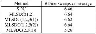
Table 3 shows the average number of fine level sweeps over all timesteps required by SDC and MLSDC to converge. The configurations MLSDC(1,2), MLSDC(1,2,3(1)) and MLSDC(1,2,3(2)) do not reduce the number of sweeps, but instead lead to a small increase. Avoiding a coarsened spatial mesh in MLSDC(2,3(1)), however, saves a small amount of fine sweeps compared to SDC. Note that here, in contrast to the example presented in§3.4, Strategy 1 has a significant negative impact on the performance of MLSDC. This illustrates that coarsening in MLSDC cannot be used in the same way for every problem: a careful adaption of the employed strategies to the problem at hand is necessary.

Method # Fine sweeps on average

SDC 6.46

MLSDC(1,2) 6.64

MLSDC(1,2,3(1)) 6.62

MLSDC(1,2,3(2)) 6.64

MLSDC(2,3(1)) 5.26

Table 3:Average number of fine level sweeps required to converge for SDC and MLSDC for the shear layer instability. The numbers indicate the different coarsening strategies.

3.4 Three-dimensional viscous Burgers’ equation

To demonstrate that MLSDC can not only reduce iterations but also runtime, we consider viscous Burgers’ equation in three dimensions

ut(x,t) +u(x,t)·∇u(x,t) =ν∇2u(x,t), x∈[0,1]3, 0≤t≤1 withx= (x,y,z), initial value

u(x,t) =exp

−(x−0.5)

2_{+ (y−0.5)}2_{+ (z−0.5)}2

σ2

homogeneous Dirichlet boundary condition and diffusion coefficientsν=0.1 andν=1.0. The problem is solved using aFORTRANimplementation of MLSDC combined with aC implementation of a parallel multigrid solver (PMG) in space [4]. A single timestep of length ∆t=0.01 is performed with MLSDC, corresponding to CFL numbers from the diffusive term on the fine level, that is

Cdiff:=

ν∆t

∆x2,

of aboutCdiff=66 (forν=0.1) andCdiff=656 (forν=1.0). The diffusion term is

inte-grated implicitly using PMG to solve the corresponding linear system and the advection term is treated explicitly. Simulations are run on 512 cores on the IBM BlueGene/Q JUQUEEN at the J¨ulich Supercomputing Centre.

MLSDC is run withM+1=3,M+1=5 andM+1=7 Gauss-Lobatto nodes with a tolerance for the residual of 10−5. Two MLSDC levels are used with all three types of coarsening applied:

1. The fine level uses a 2553point mesh and the coarse level 1273.

2. A 4th-order compact difference stencil for the Laplacian and a 5th-order WENO [27] for the advection term are used on the fine level; a 2nd_{-order stencil for the Laplacian and a}

1st_{-order upwind scheme for advection on the coarse.}

3. The accuracy of the implicit solve on the coarse level is varied by fixing the number of V-cycles of PMG on this level.

Three runs are performed, each with a different number of V-cycles on the coarse level. In the first run, the coarse level linear systems are solved to full accuracy, whereas the second and third runs use one and two V-cycles of PMG on the coarse level, respectively, instead of solving to full accuracy. These cases are referred to as MLSDC(1,2), MLSDC(1,2,3(1)), and MLSDC(1,2,3(2)). On the fine level, implicit systems are always solved to full accuracy (the PMG multigrid iteration reaches a tolerance of reach a tolerance of 10−12_{or stalls).}

Required iterations and runtimes. Table 4 shows both the required fine level sweeps for

SDC and MLSDC as well as the total runtimes in seconds for ν=0.1 and ν=1.0 for three different values ofM. MLSDC(1,2) and MLSDC(1,2,3(2)) in all cases manage to significantly reduce the number of fine sweeps required for convergence in comparison to single-level SDC, typically by about a factor of two. These savings in fine level sweeps translate into runtime savings on the order of 30−40%. For 3 and 5 quadrature nodes, there is no negative impact in terms of additional fine sweeps by using a reduced implicit solve on the coarse level and MLSDC(1,2,3(2)) is therefore faster than MLSDC(1,2). However, since coarse level V-cycles are very cheap due to spatial coarsening, the additional savings in runtime are small. For 7 quadrature nodes, using a reduced implicit solve on the coarse level in MLSDC(1,2,3(2)) comes at the price of an additional MLSDC iteration and therefore, MLSDC(1,2) is the fastest variant in this case.

M+1=3Gauss-Lobatto nodes

ν=0.1

Method F-Sweeps Runtime (sec)

SDC 9 39.4

MLSDC(1,2) 4 26.2

MLSDC(1,2,3(2)) 4 25.6

MLSDC(1,2,3(1)) 5 29.7

ν=1.0

Method F-Sweeps Runtime (sec)

SDC 16 74.1

MLSDC(1,2) 8 49.1

MLSDC(1,2,3(2)) 8 47.0

MLSDC(1,2,3(1)) 8 46.7

M+1=5Gauss-Lobatto nodes

ν=0.1

Method F-Sweeps Runtime (sec)

SDC 7 59.5

MLSDC(1,2) 3 40.8

MLSDC(1,2,3(2)) 3 39.8

MLSDC(1,2,3(1)) 8 79.7

ν=1.0

Method F-Sweeps Runtime (sec)

SDC 18 162.7

MLSDC(1,2) 9 105.6

MLSDC(1,2,3(2)) 9 101.5

MLSDC(1,2,3(1)) 14 142.8

M+1=7Gauss-Lobatto nodes

ν=0.1

Method F-Sweeps Runtime (sec)

SDC 5 82.4

MLSDC(1,2) 2 46.1

MLSDC(1,2,3(2)) 3 57.2

MLSDC(1,2,3(1)) 11 147.2

ν=1.0

Method F-Sweeps Runtime (sec)

SDC 17 224.7

MLSDC(1,2) 8 139.5

MLSDC(1,2,3(2)) 9 148.1

MLSDC(1,2,3(1)) 44 560.4

Table 4:Number of required fine level sweeps and resulting runtimes in seconds by SDC and MLSDC for 3D viscous Burgers’ equation. The numbers in parentheses after MLSDC indicate the employed coarsening strategies, see§2.2.4. Reduced implicit solves are indicated by 3(n)wherenindicates the fixed number of multigrid V-cycles. Otherwise, PMG iterates until a residual of 10−12_{is reached or the iteration stalls. The}

tolerance for the SDC/MLSDC iteration is 10−5_.

4 Discussion

The paper analyzes the multi-level spectral deferred correction method (MLSDC), an exten-sion to the original single-level spectral deferred corrections (SDC) as well as ladder SDC methods. In contrast to SDC, MLSDC performs correction sweeps in time on a hierarchy of discretization levels, similar to V-cycles in classical multigrid. An FAS correction is used to increase the accuracy on coarse levels. The paper also presents a new procedure to incor-porate weighting matrices arising in higher-order compact finite difference stencils into the SDC method. The advantage of MLSDC is that it shifts computational work from the fine level to coarse levels, thereby reducing the number of fine SDC sweeps and, therefore, the time-to-solution.

One potential continuation of this work is to investigate reducing the accuracy of im-plicit solves on the fine level in MLSDC as well. In [40], so calledinexactspectral deferred corrections (ISDC) methods are considered, where implicit solves at each SDC node are replaced by a small number of multigrid V-cycles. As with MLSDC, the reduced cost ofx implicit solves are somewhat offset by an increase in the number of SDC iterations required for convergence. Nevertheless, numerical results in [40] demonstrate an overall reduction of cost for ISDC methods versus SDC for certain test cases. The optimal combination of coars-ening and reducing V-cycles for SDC methods using multigrid for implicit solves appears to be problem-dependent, and an analysis of this topic is in preparation.

The MLSDC algorithm has also been applied to Adaptive Mesh Refinement (AMR) methods popular in finite-volume methods for conservative systems. In the AMR + MLSDC algorithm, each AMR level is associated with its own MLSDC level, resulting in a hierar-chy of hybrid space/time discretizations with increasing space/time resolution. When a new (high resolution) level is added to the AMR hierarchy, a new MLSDC level is created. The resulting scheme differs from traditional sub-cycling AMR time-stepping schemes in a few notable aspects: fine level sub-cycling is achieved through increased temporal resolution of the MLSDC nodes; flux corrections across coarse/fine AMR grid boundaries are naturally incorporated into the MLSDC FAS correction; fine AMR ghost cells eventually become high-order accurate through the iterative nature of MLSDC V-cycling; and finally, the cost of implicit solves on all levels decreases with each MLSDC V-cycle as initial guesses im-prove. Preliminary results suggest that the AMR+MLSDC algorithm can be successfully applied to the compressible Navier-Stokes equations with stiff chemistry for the direct nu-merical simulation of combustion problems. A detailed description of the AMR+MLSDC algorithm with applications is currently in preparation.

Finally, the impact and performance of the coarsening strategies presented here are also of relevance to the parallel full approximation scheme in space and time (PFASST) [17, 18, 34, 39] algorithm, which is a time-parallel scheme for ODEs and PDEs. Like MLSDC, PFASST employs a hierarchy of levels but performs SDC sweeps on multiple time intervals concurrently with corrections to initial conditions being communicated forward in time dur-ing the iterations. Parallel efficiency in PFASST can be achieved because fine SDC sweeps are done in parallel while sweeps on the coarsest level are in essence done serially. In the PFASST algorithm, there is a trade-off between decreasing the cost on coarse levels to im-prove parallel efficiency and retaining good accuracy on the coarse level to minimize the number of parallel iterations required to converge. In [18] it was shown that, for mesh-based PDE discretizations, using a spatial mesh with fewer points on the coarse level in conjunc-tion with a reduced number of quadrature nodes, led to a method with significant parallel speed up. Incorporating the additional coarsening strategies presented here for MLSDC into PFASST would further reduce the cost of coarse levels, but it is unclear how this might translate into an increase in the number of parallel PFASST iterations required.

Acknowledgements The plots were generated with the Python Matplotlib [26] package. The final publica-tion is available at springerlink.com, see http://dx.doi.org/10.1007/s10543-014-0517-x.

References

1. Alam, J.M., Kevlahan, N.K.R., Vasilyev, O.V.: Simultaneous spacetime adaptive wavelet solution of nonlinear parabolic differential equations. Journal of Computational Physics214(2), 829 – 857 (2006). 2. Ascher, U.M., Petzold, L.R.: Computer Methods for Ordinary Differential Equations and

3. B¨ohmer, K., Hemker, P., Stetter, H.J.: The defect correction approach. In: K. B¨ohmer, H.J. Stetter (eds.) Defect Correction Methods. Theory and Applications, pp. 1–32. Springer-Verlag (1984)

4. Bolten, M.: Evaluation of a multigrid solver for 3-level Toeplitz and circulant matrices on Blue Gene/Q. In: K. Binder, G. M¨unster, M. Kremer (eds.) NIC Symposium 2014, pp. 345–352. John von Neumann Institute for Computing (2014). (to appear)

5. Bourlioux, A., Layton, A.T., Minion, M.L.: High-order multi-implicit spectral deferred correction meth-ods for problems of reactive flow. Journal of Computational Physics189(2), 651–675 (2003)

6. Bouzarth, E.L., Minion, M.L.: A multirate time integrator for regularized stokeslets. Journal of Compu-tational Physics229(11), 4208–4224 (2010)

7. Brandt, A.: Multi-level adaptive solutions to boundary-value problems. Math. Comp.31(138), 333–390 (1977)

8. Briggs, W.L.: A Multigrid Tutorial. SIAM, Philadelphia, PA (1987)

9. Chorin, A.J., Marsden, J.E.: A mathematical introduction to fluid mechanics, 2nd edn. Springer-Verlag (1990)

10. Chow, E., Falgout, R.D., Hu, J.J., Tuminaro, R.S., Yang, U.M.: A survey of parallelization techniques for multigrid solvers. In: Parallel Processing for Scientific Computing, SIAM Series of Software, Envi-ronements and Tools. SIAM (2006)

11. Christlieb, A., Morton, M., Ong, B., Qiu, J.M.: Semi-implicit integral deferred correction constructed with additive Runge–Kutta methods. Communications in Mathematical Science9(3), 879–902 (2011). 12. Christlieb, A., Ong, B., Qiu, J.M.: Comments on high-order integrators embedded within integral

de-ferred correction methods. Communications in Applied Mathematics and Computational Science4(1), 27–56 (2009).

13. Christlieb, A., Ong, B.W., Qiu, J.M.: Integral deferred correction methods constructed with high order Runge-Kutta integrators. Mathematics of Computation79, 761–783 (2010).

14. Dai, X., Le Bris, C., Legoll, F., Maday, Y.: Symmetric parareal algorithms for hamiltonian systems. ESAIM: Mathematical Modelling and Numerical Analysis47, 717–742 (2013).

15. Daniel, J.W., Pereyra, V., Schumaker, L.L.: Iterated deferred corrections for initial value problems. Acta Cient. Venezolana19, 128–135 (1968)

16. Dutt, A., Greengard, L., Rokhlin, V.: Spectral deferred correction methods for ordinary differential equa-tions. BIT Numerical Mathematics40(2), 241–266 (2000)

17. Emmett, M., Minion, M.L.: Efficient implementation of a multi-level parallel in time algorithm. In: Proceedings of the 21st International Conference on Domain Decomposition Methods, Lecture Notes in Computational Science and Engineering (2012). (In press)

18. Emmett, M., Minion, M.L.: Toward an efficient parallel in time method for partial differential equations. Communications in Applied Mathematics and Computational Science7, 105–132 (2012).

19. Hagstrom, T., Zhou, R.: On the spectral deferred correction of splitting methods for initial value prob-lems. Communications in Applied Mathematics and Computational Science1(1), 169–205 (2006). 20. Hairer, E., Norsett, S.P., Wanner, G.: Solving Ordinary Differential Equations I, Nonstiff Problems.

Springer-Verlag, Berlin (1987)

21. Hairer, E., Wanner, G.: Solving Ordinary Differential Equations II, Stiff and Differential-Algebraic Prob-lems. Springer-Verlag, Berlin (1991)

22. Hansen, A.C., Strain, J.: Convergence theory for spectral deferred correction. Preprint (2006) 23. Haut, T., Wingate, B.: An asymptotic parallel-in-time method for highly oscillatory PDEs. SIAM Journal

on Scientific Computing (2014). In press

24. Huang, J., Jia, J., Minion, M.: Accelerating the convergence of spectral deferred correction methods. Journal of Computational Physics214(2), 633–656 (2006)

25. Huang, J., Jia, J., Minion, M.: Accelerating the convergence of spectral deferred correction methods. Journal of Computational Physics214(2), 633 – 656 (2006).

26. Hunter, J.D.: Matplotlib: A 2D graphics environment. Computing In Science & Engineering9(3), 90–95 (2007)

27. Jiang, G.S., Shu, C.W.: Efficient implementation of weighted ENO schemes. Journal of Computational Physics126, 202–228 (1996)

28. Layton, A.T.: On the efficiency of spectral deferred correction methods for time-dependent partial dif-ferential equations. Applied Numerical Mathematics59(7), 1629 – 1643 (2009).

29. Layton, A.T., Minion, M.L.: Conservative multi-implicit spectral deferred correction methods for react-ing gas dynamics. Journal of Computational Physics194(2), 697–715 (2004)

30. Layton, A.T., Minion, M.L.: Implications of the choice of quadrature nodes for Picard integral deferred corrections methods for ordinary differential equations. BIT Numerical Mathematics45, 341–373 (2005) 31. Lele, S.K.: Compact finite difference schemes with spectral-like resolution. Journal of Computational

32. Minion, M.L.: Semi-implicit spectral deferred correction methods for ordinary differential equations. Communications in Mathematical Sciences1(3), 471–500 (2003)

33. Minion, M.L.: Semi-implicit projection methods for incompressible flow based on spectral deferred cor-rections. Applied numerical mathematics48(3), 369–387 (2004)

34. Minion, M.L.: A hybrid parareal spectral deferred corrections method. Communications in Applied Mathematics and Computational Science5(2), 265–301 (2010).

35. Pereyra, V.: Iterated deferred corrections for nonlinear operator equations. Numerische Mathematik10, 316–323 (1966)

36. Pereyra, V.: On improving an approximate solution of a functional equation by deferred corrections. Numerische Mathematik8, 376–391 (1966)

37. Ruprecht, D., Krause, R.: Explicit parallel-in-time integration of a linear acoustic-advection system. Computers & Fluids59(0), 72 – 83 (2012).

38. South, J.C., Brandt, A.: Application of a multi-level grid method to transonic flow calculations. In: Transonic flow problems in turbomachinery, pp. 180–206. Hemisphere (1977)

39. Speck, R., Ruprecht, D., Krause, R., Emmett, M., Minion, M., Winkel, M., Gibbon, P.: A massively space-time parallel N-body solver. In: Proceedings of the International Conference on High Performance Computing, Networking, Storage and Analysis, SC ’12, pp. 92:1–92:11. IEEE Computer Society Press, Los Alamitos, CA, USA (2012).

40. Speck, R., Ruprecht, D., Minion, M., Emmett, M., Krause, R.: Inexact spectral deferred corrections using single-cycle multigrid (2014). ArXiv:1401.7824 [math.NA]

41. Spotz, W.F., Carey, G.F.: A high-order compact formulation for the 3D poisson equation. Numerical Methods for Partial Differential Equations12(2), 235–243 (1996)

42. Stetter, H.J.: Economical global error estimation. In: R.A. Willoughby (ed.) Stiff Differential Systems, pp. 245–258 (1974)

43. Trottenberg, U., Oosterlee, C.W.: Multigrid: Basics, Parallelism and Adaptivity. Academic Press (2000) 44. Weiser, M.: Faster SDC convergence on non-equidistant grids with DIRK sweeps (2013). ZIB Report

13–30

45. Xia, Y., Xu, Y., Shu, C.W.: Efficient time discretization for local discontinuous galerkin methods. Dis-crete and Continuous Dynamical Systems – Series B8(3), 677 – 693 (2007).