Seismic waveforms and velocity model heterogeneity: towards full-waveform microseismic location algorithm

This is a repository copy of Seismic waveforms and velocity model heterogeneity: towards full-waveform microseismic location algorithm.

White Rose Research Online URL for this paper: http://eprints.whiterose.ac.uk/81224/

Version: Accepted Version

Article:

Angus, DAC, Aljaafari, A, Usher, P et al. (1 more author) (2014) Seismic waveforms and velocity model heterogeneity: towards full-waveform microseismic location algorithm. Journal of Applied Geophysics, 111. 228 - 233. ISSN 0926-9851

https://doi.org/10.1016/j.jappgeo.2014.10.013

eprints@whiterose.ac.uk https://eprints.whiterose.ac.uk/ Reuse

Unless indicated otherwise, fulltext items are protected by copyright with all rights reserved. The copyright exception in section 29 of the Copyright, Designs and Patents Act 1988 allows the making of a single copy solely for the purpose of non-commercial research or private study within the limits of fair dealing. The publisher or other rights-holder may allow further reproduction and re-use of this version - refer to the White Rose Research Online record for this item. Where records identify the publisher as the copyright holder, users can verify any specific terms of use on the publisher’s website.

Takedown

If you consider content in White Rose Research Online to be in breach of UK law, please notify us by

Seismic waveforms and velocity model

heterogeneity: Towards a full-waveform

microseismic location algorithm.

D.A. Angus1, A. Aljaafari2, P. Usher3, and J.P. Verdon3 4

1

Centre for Integrated Petroleum Engineering & Geoscience, University of Leeds, UK (d.angus@leeds.ac.uk) 5

2

School of Earth & Environment, University of Leeds, UK 6

3

Department of Earth Sciences, University of Bristol, UK 7

ABSTRACT

8

Seismic forward modeling is an integral component of microseismic location

9

algorithms, yet there is generally no one correct approach, but rather a range of

10

acceptable approaches that can be used. Since seismic signals are band limited, the

11

length scale of heterogeneities can significantly influence the seismic wavefronts and

12

waveforms. This can be especially important for borehole microseismic monitoring,

13

where subsurface heterogeneity can be strong and/or vary on length scales

14

equivalent to or less than the dominant source wavelength. In this paper, we show

15

that ray-based approaches are not ubiquitously suitable for all borehole microseismic

16

applications. For unconventional reservoir settings, ray-based algorithms may not be

17

suitably accurate for advanced microseismic imaging. Here we focus on exploring the

18

feasibility of using one-way wave equations as forward propagators for full waveform

19

event location techniques. As a feasibility study, we implement an acoustic

wide-20

angle wave equation and use a velocity model interpolation approach to explore the

21

computational efficiency and accuracy of the solution. We compare the results with

22

an exact solution to evaluate travel-time and amplitude errors. The results show that

23

accurate travel-times can be predicted to within 2 ms of the true solution for modest

24

velocity model interpolation. However, for accurate amplitude prediction or for higher

dominant source frequencies, a larger number of velocity model interpolations is

1

required.

2

1. Introduction

3

Microseismic monitoring is being applied increasingly in the hydrocarbon industry

4

and this is because it provides a means of remotely monitoring the state of stress

5

(i.e. failure) within the subsurface. Microseismic technology enables monitoring

6

hydraulic fracture programs in unconventional reservoirs, assessment of fault

7

reactivation and hydrocarbon leakage in conventional reservoirs, as well as

8

characterization of the subsurface rock mass (e.g., frequency dependent seismic

9

anisotropy). Although there has been significant development of advanced

10

microseismic attributes (commonly referred to as Ôbeyond the dots in the boxÕ by

11

Eisner et al., 2010a), the location of microseismic events (the ÔdotsÕ) represent the

12

most fundamental measurement in microseismic monitoring (e.g., Eisner et al.,

13

2010b).

14

Ray based solutions, such as eikonal solvers, are very attractive since they provide

15

computationally fast solutions. If first-order effects of material averaging (or wavefront

16

smoothing) can be modelled by a gradually varying medium and the wave path

17

lengths are not too great, then basic ray methods should be applicable (e.g.,

18

Cerveny, 2001). However, ray based approaches are approximate solutions and do

19

not accurately model wave phenomena when velocity heterogeneity varies on length

20

scales on the order of or less than the dominant seismic wavelength (e.g., Cerveny,

21

2001; Angus, 2014). For instance, if strong multiple scattering or wideÐangle

22

diffraction is important, where seismic energy is scattered away from the direct ray

23

path yet in the forward direction within the Fresnel zone, a numerical solution of the

full wave equation is necessary (e.g., Thomson, 1999; Carcione et al., 2002). Full

1

waveform approaches, such as finite-difference solvers, yield substantially more

2

accurate solutions, but at the expense of slower computation times (e.g., Thomson,

3

1999). These full waveform solutions will yield very accurate solutions but, more

4

often than not, may not be practical for microseismic processing. Thus, selecting an

5

appropriate method involves weighing the advantages and disadvantages of all

6

acceptable approaches in terms of accuracy requirements and computational

7

limitations.

8

Usher et al. (2013) showed that microseismic waveforms are sensitive to velocity

9

model and microseismic source frequency (this is fundamental to the physics wave

10

propagation of bandlimited signals, i.e., frequency dependence of wave propagation).

11

This dependence on velocity model and source frequency as well as unavoidable

12

uncertainty in true velocity model will impact on the accuracy of microseismic event

13

locations and hence reliability of any geometrical interpretation (Thornton, 2013). For

14

instance, Thornton (2013) compared microseismic travel-time predictions between an

15

acoustic eikonal solver and a finite-difference solver, and observed noticeable

16

mismatch between the two solutions. The results from Thornton (2013) are

17

consistent with Usher et al. (2013) in that wave propagation is sensitive to velocity

18

model heterogeneity, and that certain ray based approaches, being limited to

19

smoothly varying velocity models, may not be universally suitable in all

20

unconventional hydrocarbon settings. Ray based approaches neglect

frequency-21

dependent effects and non-geometrical arrivals (e.g., head waves), and are generally

22

only suitable for smooth velocity models (i.e., when heterogeneity length scales are

23

greater than the dominant seismic wavelength).

In this paper, we explore the feasibility of using the wide-angle one-way wave

1

equation as a forward propagator (i.e., GreenÕs function) for microseismic event

2

location. The wide-angle one-way wave equation is capable of modeling the

3

waveform evolution along the underlying wavefront, where frequency dependent

4

effects and non-geometrical arrivals can be predicted. We focus on borehole

5

microseismic monitoring geometry, where wave propagation is predominantly

sub-6

horizontal. In such circumstances, the influence of non-geometrical arrives due to

7

horizontal layering as well as other wave phenomena due to velocity heterogeneity

8

on lengths scales on the order of or less than the dominant seismic wavelength will

9

be significant. For surface microseismic monitoring, the influence of vertical velocity

10

variation is less problematic and so ray-based methods should be appropriate.

11

2. Theory

12

2.1 The influence of GreenÕs function on event location error 13

To highlight the impact of velocity model and bandlimited wave propagation on

14

microseismic waveforms and hence on event location uncertainty, we evaluate the

15

influence of velocity model heterogeneity on event location using a ray-based

16

location algorithm. Specifically, we use an eikonal solver to generate a look-up table

17

for P- and S-wave travel-times through three depth-dependent 2D velocity models,

18

thereby providing more realistic estimates of location error. A total of nine synthetic

19

datasets are generated (Usher et al., 2013) by varying the velocity model and event

20

dominant source frequency: three velocity models (3 layer surface seismic, 13 layer

21

VSP and 34 layer sonic velocity models) and three geometrically equivalent

22

microseismic events but with different dominant source frequencies (40 Hz, 150 Hz

23

and 300 Hz). To generate the full waveform synthetics, we use the full waveform E3D

code (Larsen and Harris, 1993). E3D is a staggered grid, fourth-order accurate in

1

space and second-order accurate in time finite-difference algorithm (e.g., Virieux,

2

1984; 1986) for isotropic two-dimensional (2D) and three-dimensional (3D)

3

viscoelastic media. The specific eikonal solver used was developed as part of the

4

Madagascar package (Sethian, 1996; Sethian and Popovici, 1999). The eikonal

5

solver is used to generate a look-up table of travel-times from each point in a

6

discretized velocity model to each receiver. The optimum event location and

7

uncertainty is evaluated using the neighbourhood algorithm of Sambridge (1999a,b).

8

The root-mean-square misfit between observed travel-time from the full waveform

9

synthetic seismograms and the predicted travel-time from the ray-base eikonal solver

10

is the objective function that is minimized. Since the eikonal solver produces

travel-11

times for discrete points in the subsurface and the neighbourhood algorithm requires

12

the computation of a continuously varying hyper-surface, we use the interpolation

13

algorithm of (Akima, 1978) to compute travel-times for points between the discretized

14

grid of the eikonal solver.

15

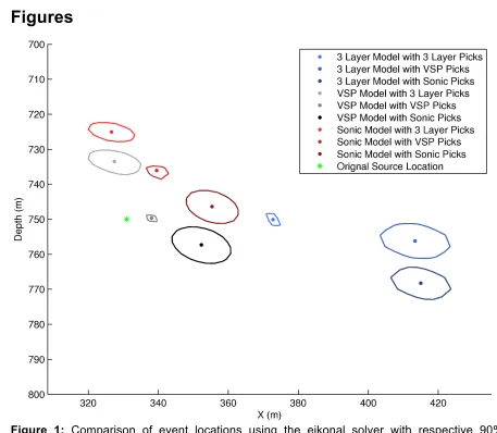
In figure 1, we compare the influence of velocity model on event location for a

16

microseismic source with dominant frequency 300 Hz (the results for lower dominant

17

frequencies are similar). In this comparison, finite-difference synthetic microseismic

18

waveforms are generated for three velocity models (3 layer surface seismic model,

19

VSP and sonic log). The travel-times of the P- and S-waves are picked manually for

20

each waveform data set. Locations for each of these sets of picks were computed

21

using an eikonal solver using each of the three velocity models, giving a total of 9

22

permutations (3 velocity models used to generate synthetic data and 3 velocity

23

models used in the event location algorithm). The resulting event locations are listed

24

in Table 1.

[Figure 1 here]

1

First we consider the cases where the velocity model used to generate the synthetic

2

data and the velocity model used to locate the events are identical (light blue,

3

medium grey and dark red dots in Figure 1). These results indicate the accuracy of

4

the location algorithm, as any mislocation will come either from errors in picking, or

5

from limitations in the use of eikonal solvers to compute travel-times: for instance,

6

eikonal solvers compute the first arrival travel-time, regardless of whether this arrival

7

is the most energetic arrival. For this case the locations are to within ± 5 m in depth.

8

The horizontal distances range between 10 m and 40 m away from the modelled

9

source location and this is due to the effects of array geometry; we use a single

10

vertical borehole in this case. Using one or more additional boreholes would improve

11

the horizontal location misfit (e.g., Jones et al., 2014). Note that for the sonic log

12

model (dark red dot in Figure 1), the confidence ellipse is larger indicating that the

13

eikonal solver is yielding less accurate results as expected given that the model

14

heterogeneity is beyond the ray theory high-frequency assumption. Next, we

15

consider the cases where one velocity model has been used to generate the full

16

waveform synthetic data, but the locations are computed using a different, and

17

therefore incorrect, velocity model. The estimated source depths range between 5 m

18

and 30 m of the true source depth, whereas the estimated source lateral locations

19

range between 10 is 90 m from the true source lateral location. This suggests there is

20

an error due to using different velocity models on the order of 10 m. We should note

21

that this error is very optimistic (i.e., best case scenario) and we would expect error in

22

real data to be larger, and this is because the synthetic waveforms are clean from

23

typical microseismic noise.

24

[Table 1 here]

2.2 Beyond ray-based algorithms Ð wide-angle one-way wave equation 1

Ray based forward modeling algorithms are extremely pervasive throughout the

2

hydrocarbon industry because they provide very efficient travel-time predictions for a

3

range of problems, such as velocity model building (e.g., Jones 2010) and event

4

locations (e.g., Maxwell 2014). However, ray theory is a high-frequency approximate

5

solution to the wave equation (Cerveny 2001) and care must be taken when applying

6

ray-based approaches to unconventional environments. Implicit in ray theory is the

7

assumption that the velocity model heterogeneity is smoothly varying with respect to

8

the length scales of the seismic wave. For microseismic events, assuming dominant

9

frequencies ranging between tens of Hz up to hundreds of Hz (e.g., Gibowicz and

10

Kijko, 1994; Trifu et al., 2000; Teanby et al., 2004; Rentsch et al., 2007; Maxwell,

11

2014), the wavelength of microseismic waves can range on the order of 100s of

12

meters for low frequency events down to 10s of meters or less for higher frequency

13

sources. For moderate to high frequency events (e.g., between 100 to 500 Hz

14

signals), vertical velocity heterogeneity can be significant enough such that the ray

15

theory assumption of smoothly varying velocity breaks-down (Thornton, 2013). This

16

is especially problematic for borehole arrays since the velocity heterogeneity varies

17

across the sub-horizontally propagating wavefront (Figure 1). However, vertical

18

heterogeneity also impacts surface array imaging, such as degrading imaging

19

aperture (e.g., Price, 2013).

20

The one-way wave equation (sometimes referred to as parabolic wave equation) has

21

been used extensively in the hydrocarbon industry primarily as a forward propagator

22

in seismic reflection migration (e.g., Claerbout, 1970) but more recently in many other

23

applications, such as modeling shear-wave splitting as well as frequency dependent

24

anisotropy (see Angus, 2014). The one-way wave equation is computationally more

efficient than full waveform solutions (e.g., finite-difference method) and this is

1

because it reduces the second-order partial differential wave equation into two

first-2

order equations (e.g., Fishmann and McCoy, 1984; Thomson, 1999; Angus, 2014).

3

This reduction to first-order with respect to a preferred axis limits one-way wave

4

equations to transmission problems, since backscatter is neglected, but allows a

5

decrease in several orders of magnitude in computational effort (see Angus 2014 for

6

review of way wave equations). In this paper, we focus on the wide-angle

one-7

way wave equation for 3-D acoustic media derived by Thomson (2005). The

wide-8

angle acoustic equation is written as

9

! !_!! !! !!! !!! ! !!!!

��_!!!_!

!! !��!! !_!! !!! !!! ! , (1)

10

where φ is the acoustic wavefield, ε is the incremental extrapolation step length in the

11

x1 direction, xα are the lateral coordinates (i.e., α=2,3), ω is frequency and p is

12

slowness. The phase propagator coefficient P1 is defined as

13

!_! !

!! !!! !! ! !

! !_!!!! !! ! ! !

!!!

, (2)

14

where v(x1,x_α) is the 3D variable acoustic velocity. The transmission coefficient Q is

15

the energy flux term

16

! !

!! !!! !_! !!!!!!

!!! , (3)

17

that enables correctly modeling the true amplitude in the presence of strong velocity

18

gradients.

19

Although equation 1 can be considered computationally efficient when compared to

20

more complete full-waveform methods, such as finite-difference methods, it is still

21

computationally cumbersome, especially for 3D media. One of the significant

22

computational costs of this algorithm stems from the shuttling between the space and

wave number domains (see Thomson, 2005); for many algorithms, this shuttling is

1

done via very efficient fast Fourier transforms (FFTs). Improvements can be made by

2

implementing theoretical approximations (Ferguson and Margrave, 2005) or by

3

manipulating model parameterization (Gazdag and Sguazzero, 1984; Thomson,

4

2005).

5

To make the implementation of equation 1 computationally efficient, we make use of

6

the velocity model interpolation concept introduced by Gazdag and Sguazzero

7

(1984). Specifically, rather than having to compute an FFT at each grid point within

8

the computational domain for each extrapolation step, an FFT is performed for an

9

integer number of velocities. For each grid point, the wavefield is computed by

10

linearly interpolating the wavefields from the nearest velocity values greater than and

11

less than the individual grid velocity value. To do this, we introduce an automated

12

linear interpolation scheme (Angus, 2014). In this approach, at each x1+ε/2 plane the

13

acoustic velocity model is discretized into i=(1, N) velocities

14

!_!∀# !

!! !!!! !! ! !! ! !��� !_!! !!!! !! , (4)

15

where Vmin and Vmax are the minimum and maximum acoustic velocities within the

16

chosen velocity model, respectively. Next, the propagator P1 and transmission

17

coefficient Q are evaluated for each discrete velocity Vi. Then N acoustic wavefields

18

φi(x1+ε; ω) are evaluated for each discrete velocity Vi using the wide-angle equation

19

1. Finally, for each lateral xα grid point, the complete wavefield φi(x1+ε; xα, pα; ω) is

20

synthesized using the linear velocity wavefield interpolation (LVWI) scheme

21

! !_!! !! !!! !!! ! ! !!!! !_! ! !! ! !!! ! !!!!_!!! !_!! !! ! , (5)

22

when Vi≤ V(x1, xα) ≤ Vi+1. The linear scaling factor is

!! ! ! !

! !_!!!! !!!

!! (6)

1

and

2

!! ! !!∀# !!!!!!!!! !!!∀# !!!!!!!!!

!!! . (7)

3

3. Results

4

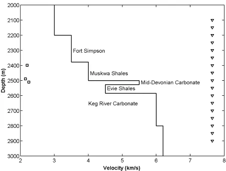
To investigate the accuracy of implementing the automated LVWI scheme (equation

5

5), we generate a suite of synthetic waveforms through the Horn River Basin velocity

6

model of Maxwell (2009). Figure 2 shows the 6-layer vertical P-wave velocity model

7

for the shale-gas reservoir, where the targets for hydraulic stimulation are the

8

Muskwa and Evie shales. To explore the accuracy of the velocity model interpolation

9

approach, we compare the travel-time and amplitude predictions from equation 5 for

10

N=2 to N=7 velocity model interpolations with the exact wide-angle equation

11

(equation 1). We compare the influence of source frequency for a range of six

12

dominant source frequencies (50, 100, 125, 150, 250 and 500 Hz) and three source

13

depths (upper shale at 2399 m, low velocity layer at 2510 m, and high velocity layer

14

at 2490 m).

15

[Figure 2 here]

16

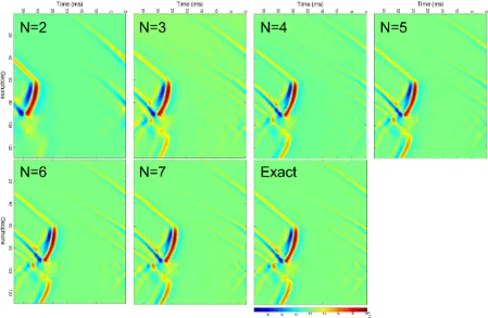
For all simulations, the wavefield is recorded along a vertical array (128 geophones

17

spaced 6.3 m vertically) giving an aperture of approximately 800 m. Figure 3 shows

18

the wavefronts and waveforms for a seismic source located at 2399 m depth and

19

having a dominant source frequency of 250 Hz. In this figure, it can be seen that as

20

the number of velocity interpolants (N) increases the level of detail in the computed

21

wavefield becomes sharper. Specifically, the computed waveforms and wavefield

22

complexity due to the low and high velocity layers become more distinct and are

much closer match to the exact solution as N increases to the total number of

1

discrete velocities (N=7).

2

[Figure 3 here]

3

The methodology used to compare the exact wide-angle wave equation predictions

4

with the various velocity model interpolations uses cross correlation to evaluate the

5

time lag between the primary arrivals. The computed time lag represents the

6

estimated travel-time error. The amplitude error is calculated after first correcting for

7

the time lag between the primary arrivals and then computing the maximum

8

amplitude of the two time-corrected arrivals. The amplitude difference is expressed in

9

terms of percentage difference from the exact wide-angle maximum amplitude.

10

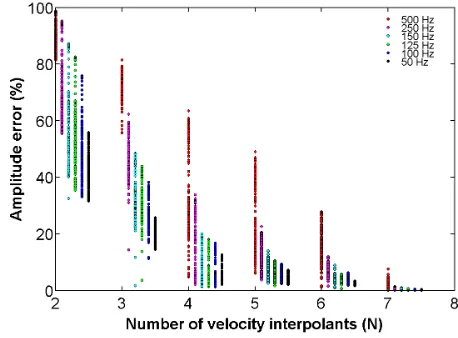
Figures 4-6 show the results of comparing the exact wide-angle solution with the

11

LVWI for the 6 velocity model interpolations (N=2 up to N=7. In Figure 4, we compare

12

the amplitude difference (error) for each velocity model interpolation for the 6

13

frequencies. Increasing the velocity interpolants from N=2 to N=7 yields improved

14

amplitude matches as expected. However, as the dominant source frequency

15

increases so does the general amplitude error.

16

[Figure 4 here]

17

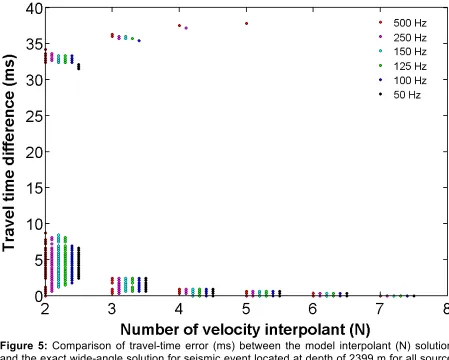
In Figure 5, travel-time differences for each velocity model interpolation with respect

18

to the exact wide-angle solution are shown for the 6 frequencies. Increasing the

19

velocity interpolants from N=2 to N=7 yields improved travel-time matches as

20

expected. For the travel-time predictions, the sensitivity to model interpolant and

21

source frequency is less severe compared to the amplitude differences shown in

22

Figure 4. At N=2, the travel-time error ranges between 5 ms and 10 ms, but for N>2

23

these errors fall below 2 ms regardless of source frequency. It should be noted that

24

the large travel-time errors computed for the low velocity model interpolant cases are

an artifact of the conventional cross-correlation technique used (e.g., Whitcombe et

1

al., 2010) related to the distorted waveforms (i.e., receivers 90 to 110 in Figure 3)

2

within the high/low velocity transition zone of the Mid-Devonian Carbonate layer and

3

the Evie Shale layer.

4

[Figure 5 here]

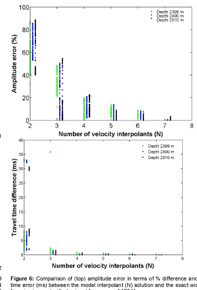
5

In Figure 6, we compare both the amplitude and travel-time differences for a 150 Hz

6

dominant source frequency event but located at three different depths; 2399 m within

7

the Muskwa shale, 2490 within the Mid-Devonian carbonate, which acts as a high

8

velocity layer, and 2510 within the Evie shale which acts as a low velocity layer (or

9

wave guide). For all depths, the general trend of improving amplitude and travel-time

10

prediction with increasing velocity model interpolant can be seen. Furthermore, there

11

appears to be no significant influence of velocity contrast above and below the

12

seismic event. Assuming travel-time picking error of 2-3 ms (e.g. Humphries, 2009;

13

Qiao and Bancroft, 2010; Kocon and van der Baan, 2012), the results from figures

4-14

6 suggest a suitable value for model interpolation would be N=3 or N=4. However, if

15

accurate amplitude information is required (e.g., for seismic moment tensor

16

inversion) then N>4 would be necessary.

17

[Figure 6 here]

18

4. Conclusions

19

We have shown that ray-based approaches are not necessarily always suitable for all

20

microseismic applications. For instance, eikonal solvers compute very effectively the

21

first arrival travel-time, regardless of whether this arrival has any energy observable

22

above the noise. Furthermore, ray based approaches assume any velocity influence

23

on travel-time is localized along the infinitely thin ray path and hence neglect velocity

averaging that bandlimited seismic waves experience. Analysis of the influence of

1

velocity model uncertainty and source frequency on location accuracy using an

2

eikonal solver will be biased by the accuracy of the approximate forward propagator

3

of the eikonal location algorithm. Thus error estimates from ray-based algorithms will

4

not necessarily convey the true error. No amount of statistical sophistication can

5

provide accurate error estimates if the forward model is not accurate enough. Thus,

6

any mislocation will come not only from errors in travel-time picking and velocity

7

model uncertainty, but also from limitations in the forward model (GreenÕs function)

8

used in the event location algorithm.

9

In this paper, we have studied the feasibility of using wide-angle one-way wave

10

equations to compute travel-time and amplitude. Although it is difficult to improve

11

velocity model uncertainty, we can certainly make improvements in the forward

12

propagator in location algorithms. Here we examine one approach to achieve

13

computational efficiency in the wide-angle wave equation and compare amplitude

14

and travel-time prediction errors to the exact wide-angle solution. The results are

15

promising considering that further computational and algorithm efficiencies can be

16

made. Although these results are applied to acoustic media, the results have

17

implications for wide-angle one-way wave equations for 3D elastic, anisotropic

18

media.

19

ACKNOWLEDGMENTS

20

The authors would like to acknowledge the sponsors of the ITF FRACGAS consortium 21

(Chevron, EBN, ExxonMobil, Marathon Oil, Nexen, Noble Energy and Total) and phases 2 22

and 3 of the BUMPS consortium (BP, Chevron, CGG, Cuadrilla, ExxonMobil, Maersk Oil, 23

Microseismic, PDO, Pinnacle, Rio Tinto, Schlumberger, Tesla, Total and Wintershall). 24

References 25

distributed data points, ACM Transactions on Mathematical Software4, 148-159, 1978. 1

Angus, D.A., The one-way wave equation: a full waveform tool for modeling seismic body 2

wave phenomena, Surveys in Geophysics, 35(2), 359-393, 2014. 3

Carcione J.S., G.C. Herman and A.P.E. ten Kroode, Y2K Review Article: Seismic modeling, 4

Geophysics, 67(4), 1304-1325, 2002. 5

Cerveny V. Seismic ray theory, Cambridge University Press, Cambridge, 2001. 6

Claerbout J., Coarse grid calculations of wave in inhomogeneous media with application to 7

delineation of complicated seismic structure, Geophysics35(3), 407-418, 1970. 8

Eisner L., Williams-Stroud S., Hill A., Duncan P. and Thornton M., Beyond the dots in the 9

box: Microseismicity-constrained fracture models for reservoir simulation, Leading Edge 10

29, 326Ð333, 2010a. 11

Eisner, L., Hulsey, B.J., Duncan, P., Jurick, D., Werner, H. and Keller, W., Comparison of 12

surface and borehole locations of induced seismicity, Geophysical Prospecting, 58, 809-13

820, 2010b. 14

Ferguson R. and Margrave G., Planned seismic imaging using explicit one-way operators, 15

Geophysics70, S101ÐS109, 2005. 16

Fishmann, L. and McCoy, J. Derivation and application of extended parabolic wave theories. 17

I. The factorized Helmholtz equation, Journal of Mathematical Physics, 25, 285Ð296. 18

1984. 19

Gazdag J. and Sguazzero P., Migration of seismic data by phase shift plus interpolation, 20

Geophysics49(2), 124-131, 1984. 21

Gibowicz S.J. and Kijko A., An introduction to mining seismology, Academic Press, 1994. 22

Humphries M., Locating VSP diffracted arrivals using a microseismic approach, SEG 23

Houston International Exposition and Annual Meeting, 4184-4188, 2009. 24

Jones, I.F. An introduction to: Velocity model building, EAGE Publications, Netherlands, 25

2010. 26

Jones, G.A., Kendall, J-M., Bastow, I.D. and Raymer, D.G., Locating microseismic events 27

using borehole data, Geophysical Prospecting, 62, 34-49, 2014. 28

Kocon K. and van der Baan M., Quality assessment of microseismic event locations and 29

traveltime picks using a multiplet analysis, The Leading Edge31(11), 1330-1346, 2012. 30

Larsen S. and Harris D., Seismic wave propagation through a low-velocity nuclear rubble 31

zone, Lawrence Livermore National Laboratory, 1993. 32

Maxwell, S., Microseismic imaging of hydraulic fracturing: Improved engineering of 33

unconventional shale reservoirs, SEG Distinguished Instructor Series, 17, 2014. 34

Maxwell, S., Microseismic location uncertainty, CSEG Recorder, April, 41-46, 2009. 35

Price, D., The effect of anhydrite on the surface imaging of microseismic events, MSc 36

dissertation, University of Leeds, 2013. 37

Qiao B. and Bancroft J.C., Picking microseismic first arrival times by Kalman filter and 38

wavelet transform, CREWES Research Report22, 2010. 39

Rentsch S., Buske S., Luth S. and Shapiro S.A., Fast location of seismicity: A migration-type 40

approach with application to hydraulic-fracturing data, Geophysics, 72(1), S33-S40, 2007. 41

Sambridge M., Geophysical inversion with a neighbourhood algorithm-I: Searching a 42

parameter space, Geophysical Journal International138, 479-494, 1999a. 43

Sambridge M., Geophysical inversion with a neighbourhood algorithm-II: Appraising the 44

ensemble, Geophysical Journal International 138, 727-746, 1999b. 45

Sethian J. and Popovici A., 3-D traveltime computation using the fast marching method, 46

Geophysics64(2), 516-523, 1999. 47

Sethian J., A fast marching level set method for monotonically advancing fronts, Proceedings 48

of the National Academy of Sciences of the United States of America 93(4), 1591-1595, 49

1996.

50

Teanby N., Kendall J-M., Jones R.H. and Barkved O., StressÐinduced temporal variations in 51

seismic anisotropy observedin microseismic data, Geophysical Journal International, 156, 52

459-466, 2004. 53

Thomson C.J., Accuracy and efficiency considerations for wide-angle wavefield extrapolators 1

and scattering operators, Geophysical Journal International163, 308-323, 2005. 2

Thomson C.J. and Chapman C.H., True-amplitude wide-angle one-way propagators and 3

high-gradient zones, EAGE 68th Conference and ExhibitionH045, Vienna, Austria, 2006. 4

Thornton M., Velocity uncertainties in surface and downhole monitoring, EAGE 4th Passive 5

Seismic WorkshopPS08, Amsterdam, Netherlands, 2013. 6

Trifu C.I., Angus D.A. and Shumila V., A Fast Evaluation of the Seismic Moment Tensor for 7

Induced Seismicity, Bulletin of the Seismological Society of America, 90(6), 1521-1527, 8

2000. 9

Usher P.J., Angus D.A. and Verdon J.P., Influence of a velocity model and source frequency 10

on microseismic waveforms: some implications for microseismic locations, Geophysical 11

Prospecting61, 334Ð345, 2013. 12

Virieux, J., SH wave propagation in heterogeneous media, velocity-stress finite difference 13

method, Geophysics, 49, 1259-1266, 1984. 14

Virieux, J., P-SV wave propagation in heterogeneous media, velocity-stress finite difference 15

method, Geophysics, 51, 889-901, 1986. 16

Whitecombe, D.N., Paramo, P., Philip, N., Toomey, A., Redshaw, T. and Linn, S., The 17

correlated leakage method Ð itÕs application to better quality timing shifts on 4D data, 72nd 18

EAGE meeting, Barcelona, Spain, Extended Abstracts, B037, 2010. 19

Tables

1

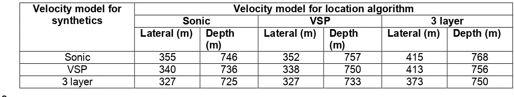
Table 1: Event locations as computed using the eikonal solver. The 3 synthetic datasets were 2

generated using the 3 velocity models. Travel-time picks for each dataset were then used to locate the 3

event using the various velocity models (yielding 9 permutations). The relative location of the event is 4

330 m horizontally (lateral distance from the well) and 750 m in depth. 5

Velocity model for synthetics

Velocity model for location algorithm

Sonic VSP 3 layer

Lateral (m) Depth (m)

Lateral (m) Depth (m)

Lateral (m) Depth (m)

Sonic 355 746 352 757 415 768

VSP 340 736 338 750 413 756

3 layer 327 725 327 733 373 750

6

Figures

1 2

3

Figure 1: Comparison of event locations using the eikonal solver with respective 90% 4

confidence ellipses for a source with dominant source frequency of 300 Hz. The true source 5

location is indicated by the green star. The blue values represent results where the synthetic 6

waveforms were generated using the 3-layer velocity model, the grey/black using the VSP 7

velocity model and the red using the sonic velocity model. The finite-difference algorithm 8

E3D is used to generate the synthetic microseismic data and the travel times from the full-9

waveform finite-difference seismograms are picked manually. The eikonal solver uses the 10

finite-difference full-waveform travel time picks to predict the event location. 11

1

Figure 2: P-wave velocity model of the Horn River Basin reservoir used in the wide-angle 2

simulations. The square symbols on the left represent the relative depth of the three seismic 3

sources. The inverted triangle symbols on the right show the relative depth extent of the 4

vertical array consisting of 128 geophones. The lateral distance between source and 5

geophone array is 250 m (not shown to scale in this figure). 6

1

Figure 3: Vertical snapshot of wavefield after propagating a total distance of 250 m 2

horizontally for N=2, 3, 4, 5, 6, and 7 number of velocity model interpolants, and the exact 3

wide-angle solution. Since the time evolution of the wide-angle solution is computed in the 4

frequency domain, the wavefield shows wrap-around in the time axis. 5

1

Figure 4: Comparison of amplitude error in terms of % difference between the model 2

interpolant (N) solution and the exact wide-angle solution for seismic event located at depth 3

of 2399 m for all source frequencies. 4

1

Figure 5: Comparison of travel-time error (ms) between the model interpolant (N) solution 2

and the exact wide-angle solution for seismic event located at depth of 2399 m for all source 3

frequencies. The large travel-time errors (between 30 and 40 ms) are due to inaccurately 4

modelled waveforms (i.e., receivers 90 to 110 in Figure 3) within the high-to-low velocity 5

transition of the Mid-Devonian Carbonate and Evie Shales (Figure 2). The waveform 6

distortion causes noticeable artifacts in the results of the conventinal cross-correlation 7

technique used. 8

1

2

Figure 6: Comparison of (top) amplitude error in terms of % difference and (bottom) travel-3

time error (ms) between the model interpolant (N) solution and the exact wide-angle solution 4

for seismic event with dominant frequency of 150 Hz. 5

6