This is a repository copy of
A quasi-Monte Carlo comparison of developments in
parametric and semi-parametric regression methods for heavy-tailed and non-normal data
: with an application to healthcare costs
.
White Rose Research Online URL for this paper:
http://eprints.whiterose.ac.uk/91029/
Version: Published Version
Article:
Jones, Andrew Michael orcid.org/0000-0003-4114-1785, Lomas, James
orcid.org/0000-0002-2478-7018, Moore, Peter et al. (1 more author) (2015) A quasi-Monte
Carlo comparison of developments in parametric and semi-parametric regression methods
for heavy-tailed and non-normal data : with an application to healthcare costs. Journal of
the Royal Statistical Society: Series A (Statistics in Society). pp. 951-974. ISSN 1467-985X
https://doi.org/10.1111/rssa.12141
[email protected] https://eprints.whiterose.ac.uk/ Reuse
Items deposited in White Rose Research Online are protected by copyright, with all rights reserved unless indicated otherwise. They may be downloaded and/or printed for private study, or other acts as permitted by national copyright laws. The publisher or other rights holders may allow further reproduction and re-use of the full text version. This is indicated by the licence information on the White Rose Research Online record for the item.
Takedown
If you consider content in White Rose Research Online to be in breach of UK law, please notify us by
2015 The Authors Journal of the Royal Statistical Society: Series A (Statistics in Society)
Published by John Wiley & Sons Ltd on behalf of the Royal Statistical Society.
This is an open access article under the terms of the Creative Commons Attribution License, which permits use, dis-tribution and reproduction in any medium, provided the original work is properly cited.
0964–1998/16/179000 J. R. Statist. Soc.A (2016)
A quasi-Monte-Carlo comparison of parametric and
semiparametric regression methods for heavy-tailed
and non-normal data: an application to healthcare
costs
Andrew M. Jones and James Lomas,
University of York, UK
Peter T. Moore
ICON Health Economics and Epidemiology, Sydney, Australia
and Nigel Rice
University of York, UK
[Received October 2014. Revised June 2015]
Summary.We conduct a quasi-Monte-Carlo comparison of the recent developments in para-metric and semiparapara-metric regression methods for healthcare costs, both against each other and against standard practice. The population of English National Health Service hospital in-patient episodes for the financial year 2007–2008 (summed for each patient) is randomly divided into two equally sized subpopulations to form an estimation set and a validation set. Evaluating out-of-sample using the validation set, a conditional density approximation estima-tor shows considerable promise in forecasting conditional means, performing best for accuracy of forecasting and among the best four for bias and goodness of fit. The best performing model for bias is linear regression with square-root-transformed dependent variables, whereas a gen-eralized linear model with square-root link function and Poisson distribution performs best in terms of goodness of fit. Commonly used models utilizing a log-link are shown to perform badly relative to other models considered in our comparison.
Keywords: Healthcare costs; Health econometrics; Heavy tails; Quasi-Monte-Carlo methods
1. Introduction
The distribution of healthcare costs provides many challenges to the applied researcher: values are non-negative (often with many observations with costs of 0), heteroscedastic, positively skewed and leptokurtic. Although these, or similar, challenges are found within many areas of empirical economics, the large interest in modelling healthcare costs has driven the development of an expanding array of estimation approaches and provides a natural context to compare methods for handling heavy-tailed and non-normal distributions. For an excellent review of statistical methods for the analysis of healthcare cost data with an emphasis on data collected alongside randomized trials, see Mihaylovaet al. (2011). Econometric models of healthcare costs include applications to risk adjustment in insurance schemes (Van de Ven and Ellis, 2000),
Address for correspondence: Nigel Rice, Centre for Health Economics, Alcuin Block A, University of York, Heslington, York,YO10 5DD, UK.
in devolving budgets to healthcare providers (e.g. Dixonet al. (2011)), in studies calculating attributable healthcare costs to specific health factors or conditions (Johnsonet al., 2003; Cawley and Meyerhoefer, 2012) and in identifying treatment costs in health technology assessments (Hochet al., 2002).
In attempting to capture the complex distribution of healthcare costs, two broad modelling approaches have been pursued. The first consists of flexible parametric models—distributions such as the three-parameter generalized gamma and the four-parameter generalized beta of the second kind distributions. This approach is attractive because of the range of distributions that these models encompass, whereas models with fewer parameters are inherently more restrictive, especially in regard to the assumptions that they impose on higher moments of the distribution (e.g. skewness and kurtosis). The second is the use of semiparametric models including extended estimating equations (EEEs), finite mixture models and conditional density approximation estimators. The EEE model adopts the generalized linear models (GLMs) framework and al-lows for the link and distribution functions to be estimated from data, rather than specified
a priori. Finite mixture models introduce heterogeneity (both observed and unobserved) through mixtures of distributions. Conditional density approximation estimators are implemented by dividing the empirical distribution into discrete intervals and then decomposing the conditional density function into ‘discrete hazard rates’. Despite the burgeoning availability of healthcare costs data via administrative records, together with an increased necessity for policy makers to understand the determinants of healthcare costs and more, it is surprising that no previous study compares comprehensively the models belonging to these two strands of literature. In this paper we compare these approaches both with each other and against standard practice: linear regression on levels, and on square-root and log-transformations, of costs and GLMs.
Traditional Monte Carlo simulation approaches would not be appropriate for such an exten-sive comparison, as we are interested in a very large number of permutations of assumptions underlying the distribution of the outcome variable. In addition, such studies are prone to affording advantage to certain models arising from the chosen distributional assumptions that are used for generating data. Instead, using a large administrative database consisting of the population of English National Health Service (NHS) hospital in-patient users for the year 2007–2008 (6 164 114 unique patients), we adopt a quasi-Monte-Carlo approach where regression models are estimated on observations from one subpopulation and evaluated on the remaining subpopulation. This enables us to evaluate the regression methods in a rigorous and consistent manner—while ensuring that results are not driven either by overfitting to rare but influential observations, or traditional Monte Carlo distributional assumptions—and are generalizable to hospital in-patient services.
This paper compares and contrasts systematically these recent developments in semi-parametric and fully semi-parametric modelling both against each other and against standard prac-tice. More strictly speaking, these recent developments are those that have featured in a Monte Carlo, cross-validation or quasi-Monte-Carlo empirical comparative study. An example of a promising method that is not compared is the extension to GLMs that was proposed by Holly
Quasi-Monte-Carlo Comparison of Parametric and Semiparametric Regression Methods 3
Under certain circumstances this is justified, for instance if the policy maker has a sufficiently large budget (Arrow and Lind, 1970). Other features of the distribution may be of interest (Van-ness and Mullahy, 2007), especially when the policy maker has a smaller budget to allocate to healthcare. Given our focus, we analyse bias, accuracy and goodness of fit of forecasted condi-tional means. We find that no model performs best across all metrics of evaluation. Commonly used approaches—linear regression on levels of costs, linear regression on log-transformed costs, the use of gamma GLMs with log-link, and the use of the log-normal distribution—are not among the four best performing approaches with any of our chosen metrics. Our results indicate that models that are estimated with a square-root link perform much better than those with log- or linear link functions. We find that linear regression with a square-root-transformed dependent variable is the best performing model in terms of bias; the conditional density approximation estimator (using a multinomial logit) for accuracy and the Poisson GLM with square-root link best in terms of goodness of fit.
2. Previous comparative studies
Various studies have compared the performance of regression-based approaches to modelling healthcare cost data, where model performance is assessed on either actual costs (i.e. costs with an unknown true distribution) (Deb and Burgess, 2003; Veazieet al., 2003; Buntin and Zaslavsky, 2004; Basuet al., 2006; Hill and Miller, 2010; Joneset al., 2014) or simulated costs from an assumed distribution (Basuet al., 2004; Gilleskie and Mroz, 2004; Manninget al., 2005). Using actual costs preserves the true empirical distribution of cost data, and all of its complexities, whereas simulating costs provides a benchmark using the known parameters of the assumed distribution (classic Monte Carlo sampling) against which models can be compared.
Studies based on the classic Monte Carlo design are therefore ideally suited to assessing whether or not regression methods can fit data when specific assumptions, and permutations thereof, are imposed or relaxed. The complexities of the observed distribution of healthcare costs are such that a comprehensive comparison of modelling approaches would require an infeasibly large number of permutations of distributional assumptions used to generate data to make a classic Monte Carlo simulation worthwhile. Choosing a subset of the possible permutations of assumptions is prone to cause bias in the results in favour of certain methods. A reliance on actual data, as an alternative approach, requires large data sets so that forecasting is evaluated on sufficient observations to reflect credibly all of the idiosyncratic features of cost data. With this approach, however, it is difficult to assess exactly which aspect of the distribution of healthcare costs is problematic for each method under comparison.
2.1. Studies using cross-validation approaches
With improvements in computational capacity, there have recently been several studies using large data sets to perform quasi-Monte-Carlo comparisons across regression models for health-care costs. Quasi-Monte-Carlo comparisons divide the data into two groups, with samples repeatedly drawn from one group and models estimated, whereas the other group is used to evaluate out-of-sample performance (using the coefficients from the estimated models). In this section, we briefly review work that has implemented quasi-Monte-Carlo comparisons (Deb and Burgess, 2003; Joneset al., 2014, 2015) as well as discuss related approaches and important results.
comprised of approximately 3 million individual records. From within these observations a subgroup of 1.5 million individual records was used as an ‘estimation’ group and another sub-group of 1 million records formed a ‘prediction’ sub-group. Their results highlight a trade-off between bias and precision, and the need for caution surrounding the use of finite mixture models at smaller sample sizes. In terms of bias, they found that linear regression (on levels and square-root-transformed levels of costs) performs best, whereas in terms of accuracy models based on a gamma density have better performance. Joneset al. (2014) focused exclusively on parametric models and suggested the use of the generalized beta of the second kind model as an appropriate distribution for healthcare costs. Their quasi-Monte-Carlo design compared this distribution together with its nested and limiting cases, including the generalized gamma model. Using data from hospital episode statistics split into ‘estimation’ and ‘validation’ sets, they found little evidence that the performance of models varies with sample size, but they found variation be-tween models in their ability to forecast mean costs, with the generalized gamma distribution the most accurate and the beta of the second kind distribution the least biased. Joneset al. (2015) also adopted the quasi-Monte-Carlo design but focused entirely on estimating and fore-casting based on the cumulative distribution function and not on the conditional mean of the distribution.
Hill and Miller (2010) and Buntin and Zaslavsky (2004) also used cross-validation techniques so that models are estimated on samples of data and evaluated on the remaining observations. Samples for estimation and the remaining data for evaluation differ across replications such that, unlike a quasi-Monte-Carlo design, individuals may fall into either the estimation sample or the validation sample at each replication. This approach is less data intensive and providing sufficient replications should produce sufficient information in the evaluation exercise to judge model performance. The approaches are similar in that they both replicate the sampling process to ensure that there is no ‘lucky split’ and guard against overfitting by evaluating out of sample. An alternative approach was considered in Veazieet al. (2003) where models were estimated on samples of observations belonging to 1992–1993 and evaluated on 1993–1994 observations. This is closer to the quasi-Monte-Carlo design and could potentially evaluate on data with a different underlying generating process, since they are from a different time period. Out-of-sample performance was also used as one metric in Basuet al. (2006) where they undertook tests of overfitting (Copas, 1983).
2.2. Recent developments in semiparametric and fully parametric modelling
Quasi-Monte-Car
lo
Compar
ison
of
P
ar
ametr
ic
and
Semipar
ametr
ic
Reg
ression
Methods
[image:6.485.77.643.142.353.2]5
Table 1. Models included in recent published comparative work
Method Studies using Monte Carlo Studies using cross-validation Studies using
quasi-Monte-methods Carlo methods
Veazie Buntin and Basu Hill and
Basu Gilleskie Manning et al. Zaslaysky et al. Miller Deb and Jones This et al. and Mroz et al. (2003) (2004) (2006) (2010) Burgess et al. study
(2004) (2004) (2005) (2003) (2013)
Linear regression
Linear regression (logarithmic)
Linear regression (square root)
Log-normal
Gaussian GLM †
Poisson
Gamma
EEE models
Weibull ‡
Generalized gamma
Generalized beta of the second kind
Finite mixture of gamma distributions
Conditional density estimator
†Not commonly used and problematic in estimation for our data in preliminary work.
Given an increasing interest in modelling healthcare costs for resource allocation, risk adjust-ment and identifying attributable treatadjust-ment costs, together with the burgeoning availability of data through administrative records, a comprehensive and systematic comparison of available approaches is timely. The results of this comparison will have resonance beyond healthcare costs and should be of interest to empirical applications to other right-skewed, leptokurtic or heteroscedastic distributions such as income and wages.
3. Specification of models
We compare 16 models that are applicable to healthcare cost data. Each makes different assump-tions about the distribution of the outcome (cost) variable. Each regression uses the same vector of covariatesXi, although the precise way in which they affect the distribution varies across mod-els. The covariates included are age, age2, age3, gender, genderÅage, genderÅage2, genderÅage3 and 24 morbidity markers indicating the presence or absence, coded 1 and 0 respectively, of one or more spells with any diagnosis within the relevant subset of version 10 international classification of diseases (ICD) codes (the 24 groupings were determined on the basis of clinical factors and initial letter of the ICD code; see the on-line appendix A for more details). All models specify at least one linear index of covariatesX′iβ. In addition, linear regression meth-ods with transformed outcome require assumptions surrounding the form of heteroscedasticity (modelled as a function ofXi), to retransform predictions onto the natural cost scale (Duan, 1983). Within the GLM family, we explicitly model the mean and variance functions as some transformation of the linear predictor (Bloughet al., 1999). Fully parametric distributions, such as the gamma and beta family of models, require an assumption about the form of the entire distribution. In this paper, a single parameter is estimated as a function of the linear index. Finite mixture models allow for multiple densities, each a function of the covariates in linear form. For conditional density approximation estimator models, the empirical distribution of costs is divided into intervals, and functions of the independent variables predict the probability of lying within each interval.
Beginning with linear regression, we estimate three models by using ordinary least squares (OLS): the first is on the level of costs; the second and third use a log- and square-root-transformed dependent variable respectively (log-transformation is more commonly used in the literature (Jones, 2011)). With these approaches, predictions are generated on a transformed scale, and it is necessary to calculate an adjustment to retransform predictions to their natural cost scale. This is done by applying a smearing factor, which varies according to covariates in the presence of heteroscedasticity (Duan, 1983). Residuals from the first regression of transformed healthcare cost against covariates are transformed by using the link function. Regressing the transformed residual against the covariates and taking these predicted values gives each obser-vation’s smearing factor.
Quasi-Monte-Carlo Comparison of Parametric and Semiparametric Regression Methods 7
the Poisson case, the variance is proportional to the conditional mean function of covariates and in the gamma case the variance is proportional to the conditional mean squared. Two of the combinations of link functions and distribution families are associated with commonly used distributions. In particular, the GLM with log-link and gamma variance is commonly applied to healthcare costs, and the GLM with a log-link and Poisson variance is associated with the Poisson model (see the discussion in Mullahy (1997)).
3.1. Flexible parametric models
Within the GLM and OLS approaches, much focus is placed on heteroscedasticity and the form that it takes. Recent developments in fully parametric modelling have been made where the modelling of higher moments, skewness and kurtosis is tackled explicitly. With this approach, the researcher estimates the entire distribution by using maximum likelihood, which requires that the distribution is correctly specified for consistent results. If the distribution is correctly specified, then estimates are efficient.
3.1.1. Generalized gamma model
We estimate two models from within the gamma family, which have typically been used for durations, but also have precedent in the healthcare costs literature (Manninget al., 2005): the log-normal and generalized gamma distributions. Each of these is estimated, using maximum likelihood, with a scale parameter specified as an exponential function of covariates, denoted exp.X′iβ/. The probability density function and conditional mean for the generalized gamma distribution are
f.yi|Xi/=
κ[κ−2{y
i=exp.X′iβ/}κ=σ]κ −2
exp [−κ−2{y
i=exp.X′iβ/}κ=σ]
σyiΓ.κ−2/
, .1/
E.yi|Xi/=exp.X′iβ/κ2
σ=κΓ.κ−2+σ=κ/
Γ.κ−2/ .2/
whereσis a scale parameter,κis a shape parameter andΓ.·/is the gamma function.
When κ→0 the generalized gamma distribution approaches the limiting case of the log-normal distribution, for which the probability density function and conditional mean are
f.yi|Xi/= 1
σyi√.2π/ exp
−{ln.yi/−X′iβ}2 2σ2
, .3/
E.yi|Xi/=exp.X′iβ/exp
σ2
2
: .4/
3.1.2. Generalized beta of the second kind distribution
We also include the generalized beta of the second kind distribution, which has yet to be com-pared with a broad range of regression models (in Joneset al. (2014), beta-type models were limited to comparison with gamma-type distributions). Beta-type models, like gamma-type models, require assumptions about the form of the entire distribution. Until recently, they have been used largely in actuarial applications, as well as for the modelling of incomes (Cummins
distribution, since all beta-type (and gamma-type) distributions are nested or limiting cases of this distribution. It therefore offers the greatest flexibility in terms of modelling healthcare costs among the duration models that are used here: see for example the implied restrictions on skew-ness and kurtosis (McDonaldet al., 2013). The probability density function and conditional mean are
f.yi/=
ayiap−1
b.Xi/apB.p,q/[1+{yi=b.Xi/}a]p+q
, .5/
E.yi|Xi/=b.Xi/
Γ.p+1=a/Γ.q−1=a/
Γ.p/Γ.q/
.6/
whereais a scale parameter,pandqare shape parameters andB.p,q/=Γ.p/Γ.q/=Γ.p+q/is the beta function.
We parameterize the generalized beta of the second kind distribution with the scale parameter
bas two different functions of covariates: a log-link and a square-root link.
3.2. Semiparametric methods
3.2.1. Extended estimating equations
A flexible extension of GLMs has been proposed by Basu and Rathouz (2005) and Basuet al. (2006), which is known as the EEE model. It approximates the most appropriate link by using a Box–Cox function, whereλ=0 implies a log-link andλ=0:5 implies a square-root link:
E.yi|Xi/=.λXi′β+1/1=λ .7/
as well as a general power function to define the variance with constant of proportionalityθ1
and powerθ2:
var.yi|Xi/=θ1E.yi|Xi/θ2: .8/
Suppose that the distribution of the outcome variable is unknown but has mean and variance nested within equations (7) and (8). An incorrectly specified GLM mean function, where com-mon usage of GLM mean functions is limited to standard forms such as log- and square-root link functions, yields biased and inconsistent estimates, whereas estimates from EEE models should be unbiased, provided that the specification of regressors is correct. A well-specified mean function combined with an incorrectly specified distribution form will be inefficient com-pared with EEE models. If the distribution is known to be a specific GLM form, the EEE model is less efficient than the appropriate GLM, but both are unbiased.
3.2.2. Finite mixture models
Finite mixture models have been employed in health economics to allow for heterogeneity both in response to observed covariates and in terms of unobserved latent classes (Deb and Trivedi, 1997). Heterogeneity is modelled through a number of components, denotedC, each of which can take a different specification of covariates (and shape parameters, where specified), written asfj.yiXi/, and where there is a parameter for the probability of belonging to each component,
πj. The general form of the probability density function of finite mixture models is
f.yi|Xi/= C
j
Quasi-Monte-Carlo Comparison of Parametric and Semiparametric Regression Methods 9
We use two gamma distribution components in our comparison. Preliminary work showed that models with a greater number of components led to problems with convergence in estima-tion. Empirical studies such as Deb and Trivedi (1997) provide support for the two-components specification for healthcare use. In one of the models used, we allow for log-links in both com-ponents (10), and in the other we allow for a square-root link (11). In both, the probability of class membership is treated as constant for all individuals and a shape parameterαjis estimated for each component:
fj.yi|Xi/=
yiαj
yiΓ.αj/exp.X′iβj/αj exp
−exp.Xyi′ iβj/
, .10/
fj.yi|Xi/=
yiαj
yiΓ.αj/.X′iβj/2αj exp
− yi
.X′iβj/2
: .11/
The conditional mean is given for the log-link specification and for the square-root link by equations (12) and (13) respectively:
E.yi|Xi/= C
j
πjαjexp.Xi′βj/, .12/
E.yi|Xi/= C
j
πjαj.X′iβj/2: .13/
Unlike the models in the previous section, this approach can allow for a multimodal distri-bution of costs. In this way, finite mixture models represent a flexible extension of parametric models (Deb and Burgess, 2003). Using increasing numbers of components, it is theoretically possible to fit any distribution, although in practice researchers tend to use few components (two or three) and achieve good approximation to the distribution of interest (Heckman, 2001).
3.2.3. Conditional density approximation estimators
Finally, we use two additional models that are applications of the conditional density approxi-mation estimator that was outlined in Gilleskie and Mroz (2004). Their method is an extension of the two-part model that is frequently used to deal with zero costs, in that the range of outcome variable is divided intoQparts (or intervals), where the mean (of observations to be used in estimation) within intervalj(j=1,: : :,Q) isyjand the lower and upper threshold values are
yj−1andyjrespectively (wherey0is equal to the lowest observed cost andyQis equal to the highest observed cost). The probability that an observation falls into intervaljcan be written as
pij.Xi/=P.yj−1yi< yj|Xi/= yj
yj−1
f.yi|Xi/dyi: .14/
The density function is then approximated byQ‘discrete hazard rates’, defined as the prob-ability of lying in intervalj conditionally on not lying in intervals 1,: : :,j−1 and written as
λ.j,Xi/:
λ.j,Xi/=P.yj−1yi< yj|Xi,yiyj−1/=
yj
yj−1
f.yi|Xi/dyi
1− yj−1
y0
f.yi|Xi/dyi
The effect of covariates can vary smoothly, or discontinuously, across intervals depending on how the model is specified: with the most flexible case using a separate model for each interval’s hazard rate. We assume that only the probability of lying within an interval depends on covariates, and that the mean value of the outcome variable, for a given interval, does not vary with covariates. The conditional mean function is therefore obtained by using
E.yi|Xi/= Q
j=1
pij.Xi/yj: .16/
One of the main benefits of this approach is the flexibility that is afforded with respect to the intervals that are used. There is flexibility in terms of the number of intervals, and where the boundaries between them are placed, as well as the degree to which the ‘discrete hazard rates’ are estimated separately for each interval. Within our illustration, we use 15 equally sized intervals across all samples. Gilleskie and Mroz (2004) in their application to healthcare costs found that between 10 and 20 intervals result in a good approximation, based on an adjusted log-likelihood to guard against overfitting, and we found that 15 intervals resulted in good convergence performance in preliminary work. In practice, a researcher would experiment with different intervals and compare model performance to decide on the specification. Having decided on the intervals to be used, we use a multinomial logit specification and an ordered logit specification to model the probabilities of lying within each interval. This differs from the less parametric single-logit specification that was adopted in Gilleskie and Mroz (2004), which is more computationally demanding, and instead uses an approach similar to that of Han and Hausman (1990). The multinomial logit specification is similar to running a separate logit model for each ‘discrete hazard rate’, whereas the ordered logit specification is analogous to allowing the discrete hazard rate to vary discontinuously for each interval but with no discontinuity in the effects of covariates. Fully adhering to Gilleskie and Mroz (2004) would allow the data to determine how flexibly to estimate the discrete hazard rates; once again our implementation is a simpler approach which approximates their method:
pij.Xi/=
exp.X′iβj/ Q
l=1
exp.X′iβl/
.17/
whereβ1=0 to normalize for estimation purposes
pij.Xi/=
exp.ψj−X′iβ/ 1+exp.ψj−X′iβ/
−pij−1 .18/
where ψj represents the estimated threshold value for each category from the ordered logit model,pi0=0 andpi15=1−pi14, so we estimate only 14 threshold values (in our application Q=15).
Conditional means from these models are calculated as in equation (16), where the probabili-tiespijare calculated by using equation (17) for the multinomial logit specification and equation (18) for the ordered logit specification.
4. Data and choice of variables
Quasi-Monte-Carlo Comparison of Parametric and Semiparametric Regression Methods 11
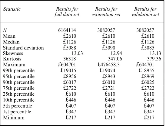
Table 2. Descriptive statistics for hospital costs
Statistic Results for Results for Results for full data set estimation set validation set
N 6164114 3082057 3082057 Mean £2610 £2610 £2610 Median £1126 £1126 £1126 Standard deviation £5088 £5090 £5085 Skewness 13:03 12:94 13:13 Kurtosis 36318 347:06 379:36 Maximum £604701 £476458:3 £604701 99th percentile £19015 £19074 £18955 95th percentile £8956 £8943 £8969 90th percentile £6017 £6010 £6025 75th percentile £2722 £2721 £2722 25th percentile £610 £610 £610 10th percentile £446 £446 £446 5th percentile £407 £407 £407 1st percentile £347 £347 £347 Minimum £217 £217 £217
hospitals (Dixonet al., 2011). For our study, we exclude spells which were primarily mental or maternity healthcare, as well as private sector spells. This data set was compiled as part of a wider project considering the allocation of NHS resources to primary care providers. Since much mental healthcare is undertaken in the community and with specialist providers, and hence is not recorded in the hospital episode statistics, the data are incomplete, and also since healthcare budgets for this type of care are constructed by using separate formulae. Maternity services are excluded since they are unlikely to be heavily determined by morbidity characteristics, and accordingly for the setting of healthcare budgets are determined by using alternative mecha-nisms. The hospital episode statistics database is a large administrative data set collected by the Health and Social Care Information Centre (now named the NHS Information Centre), with our data set comprising 6164114 separate observations, representing the population of hospital in-patient healthcare users for the year 2007–2008. Since data are taken from administrative records, we have information only on users of in-patient NHS services, and therefore we can only model strictly positive costs (0s are typically handled by a two-part specification and the main challenge is to capture the long and heavy tail of the distribution rather than the 0s).
The cost variable that is used throughout is individual patient annual NHS hospital cost for all spells finishing in the financial year 2007–2008. To cost utilization of in-patient NHS facilities, tariffs from 2008–2009 (reference costs for 2005–2006, which were the basis for the tariffs from 2008–2009, were used when 2008–2009 tariffs were unavailable) were applied to the most expensive episode within the spell of an in-patient stay (following standard practice for costing NHS activity). Then, for each patient, all spells within the financial year were summed. The data are summarized in Table 2.
Fig. 1. Variance against mean for each of the 20 quantiles of the linear index of covariates: the data were divided into 20 subsets by using the deciles of a simple linear predictor for healthcare costs with the set of regressors introduced later; the figure plots the means and variances of actual healthcare costs for each of these subsets, with fitted linear and quadratic trends
data-generating process—can be seen from the number of percentiles that are the same across both subsets.
We construct a linear index of covariates (by regressing the outcome variable on the set of covariates that we include in our regression models by using OLS) and divide the data into quantiles according to this, to analyse conditional (onX) distributions of the outcome variable. First, we plot the variances of each quantile against their means (Fig. 1). This gives us a sense both of the nature of heteroscedasticity and of feasible assumptions relating these aspects of the distribution. From Fig. 1, we can see that there is evidence against homoscedasticity (where there would be no visible trend), and evidence for some relationship between the variance and the mean. A similar analysis can be carried out for higher moments of the distribution, plotting the kurtosis of each quantile against their skewness. Parametric distributions impose restrictions on possible skewness and kurtosis: one-parameter distributions are restricted to a single point (for example a normal distribution imposes a skewness of 0 and a kurtosis of 3), two-parameter distributions allow for a locus of points to be estimated and distributions with three or more parameters allow for spaces of possible skewness and kurtosis combinations. For further details see Holly and Pentsak (2006), Pentsak (2007), McDonaldet al. (2013) and Joneset al. (2015).
Quasi-Monte-Carlo Comparison of Parametric and Semiparametric Regression Methods 13
any diagnosis within the relevant subset of ICD version 10 chapters, during the financial year 2007–2008 (see appendix A). We do not use a fully interacted specification, since morbidity is modelled with a separate intercept for the presence of each type of diagnosis (and not interacted with age or gender). However, we do allow for interactions between age and its higher orders and gender. This means that we are left with a specification that is close to those used in the comparative literature as well as a parsimonious version of the set of covariates that are used to model costs in person-based resource allocation in England, as in, for example, Dixonet al. (2011). In addition, making the specification less complicated aids computation and results in fewer models failing to converge.
5. Methodology
5.1. Quasi-Monte-Carlo design
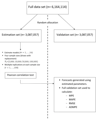
By using the hospital episode statistics data, we have access to a large amount of observations representing the whole population of English NHS in-patient costs. To exploit this, we use a quasi-Monte-Carlo design similar to that of Deb and Burgess (2003). The population of obser-vations (6 164 114) is randomly divided into two equally sized subpopulations: an estimation set (3 082 057) and a validation set (3 082 057). From within the estimation set we randomly draw, 100 times with replacement, samples of sizeNs(Ns∈5000, 10 000, 50 000, 100 000). The models are estimated on the samples and performance then evaluated on the sample drawn from both the estimation set and the full validation set. Using a split sample to evaluate models has prece-dent in the comparative literature on healthcare costs; see Duanet al. (1983) and Manninget al. (1987). Fig. 2 illustrates our study design in the form of a diagram: note that the subscriptm
denotes the model used,Nsthe sample size used andrthe replication number.
To execute this quasi-experimental design, we automate the model selection process for each approach: for instance, with the conditional density approximation estimator, we specify a number of bins to be estimated,a priori, rather than undergoing the investigative process that was outlined in Gilleskie and Mroz (2004). Similarly, all models have been automated to some extent, since we seta priorithe specification of regressors (all models), the parameters that vary with covariates (generalized gamma and generalized beta of the second kind models) and the number of mixtures to model (finite mixture models). Our specification of regressors was based on preliminary work, which showed that alternative specifications, including the use of a count of the number of morbidities, give similar results, but with worse convergence performance.
5.2. Evaluation of model performance
5.2.1. Estimation sample
Full data set (n= 6,164,114)
Random allocation
Estimation set (n= 3,087,057)
Validation set (n= 3,087,057)
Estimate models ( )
Four sample sizes (draws with replacement)
Multiple replications at each sample size
( )
Pearson correlation test
Forecasts generated using estimated parameters.
Full validation set used to calculate:
MPE
[image:15.485.74.410.53.467.2]MAPE RMSE ADMPE
Fig. 2. Diagram setting out the study design
test, residuals (computed on the raw cost scale) are regressed against predicted values of cost. If the slope coefficient on the predicted costs is significant, then this implies a detectable linear relationship between the residuals and the covariates, and so evidence of model misspecification.
5.2.2. Validation set
Quasi-Monte-Carlo Comparison of Parametric and Semiparametric Regression Methods 15
(RMSE), RMSEmsr=√{Σ.yi−yˆi/2=Ns}) of these forecasts. The MPE can be thought of as measuring the bias of predictions at an aggregate level, where positive and negative errors can cancel each other out, whereas the MAPE is a measure of the accuracy of individual predic-tions. The RMSE is similar to the MAPE in that positive and negative errors do not cancel out; however, larger errors count for disproportionately more, since they are squared. In ad-dition, we evaluate the variability of bias across replications (absolute deviations of the mean prediction error (ADMPE), ADMPEmsr= |MPEmsr−ΣRr=1MPEmsr=R|). These are all evalu-ated on the full validation set, wheremdenotes the model used,sthe sample size used andrthe replication.
Only replications where all 16 models are successfully estimated on the sample are included for evaluation, and model performance according to each criterion is calculated as an average over all included replications, e.g. MPEms=ΣRr=1MPEmsr=R. All models estimated successfully every time, except for the CDEM and EEE models. CDEM could not be estimated on two of the 100 replicates with samples of 5000 observations. The EEE models could not be estimated on four, four, six and four of the 100 replicates with sample sizes of 5000, 10 000, 50 000 and 100 000 observations respectively.
To obtain a greater insight into the performance of different distributions, we evaluate forecasted conditional means at different values of the covariates. In practice this is done by partitioning the fitted values of costs into deciles. We assess the MPE and MAPE for deciles of predicted costs, since there is concern that models perform with varying success at dif-ferent points in the distribution. Models designed for heavy tails, for instance, might be ex-pected to perform better in predicting the biggest costs. This also represents a desire to fit the distribution of costs for different groups of observations according to their observed covari-ates.
We combine the results that we obtain from different sample sizesNs and attempt to find a pattern in the way in which models perform as the sample size varies. To do this we con-struct response surfaces (as in, for example, Deb and Burgess (2003)). These are polynomial approximations to the relationship between the statistics of interest and the sample size of the experiment,Ns. For our purposes, we estimate the following regression for each model and for each metric of performance (illustrated below for the MPE):
MPEmsr=αMPEm +βmMPE 1
Ns +
uMPEmsr : .19/
We specify the relationship between the MPE and the inverse of the sample size, reflecting that we expect reduced bias as the number of observations increases. In particular, the value ofαMPEm represents the value of the MPE to which the model approaches asymptotically with increasing sample size: testing whether or not this is statistically significant from 0 gives an indication of whether the estimator is consistent. Here,uMPEmsr represents the error term from the regression. For the metrics that cannot be negative, we use the log-function of the value as the dependent variable. With the log-specification, differences in estimates are to be interpreted as percentage differences, as opposed to absolute differences.
6. Results and discussion
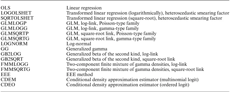
Table 3. Key for model labels
OLS Linear regression
LOGOLSHET Transformed linear regression (logarithmically), heteroscedastic smearing factor SQRTOLSHET Transformed linear regression (square-root), heteroscedastic smearing factor GLMLOGP GLM, log-link, Poisson-type family
GLMLOGG GLM, log-link, gamma-type family GLMSQRTP GLM, square-root link, Poisson-type family GLMSQRTG GLM, square-root link, gamma-type family LOGNORM Log-normal
GG Generalized gamma
GB2LOG Generalized beta of the second kind, log-link GB2SQRT Generalized beta of the second kind, square-root link FMMLOGG Two-component finite mixture of gamma densities, log-link FMMSQRTG Two-component finite mixture of gamma densities, square-root link
EEE EEE method
CDEM Conditional density approximation estimator (multinomial logit) CDEO Conditional density approximation estimator (ordered logit)
6.1. Estimation sample results
We first conduct tests of misspecification across the models used. Researchers use these tests to inform the specification of regressors, and the appropriateness of distributional assumptions, in particular the link function. Since we use the same regressors in all models, our tests are used to inform choices of distributional assumptions. The Pearson correlation coefficient test can detect whether there is a linear association between the estimated residuals and estimated conditional means, where the null hypothesis is no association. A lack of this kind of association suggests evidence against misspecification. It is also possible, however, that the relationship between the error and covariates is non-linear, which this test cannot detect. Linear regression estimated by using OLS, by construction, generates residuals that are orthogonal to predicted costs, and so the Pearson test cannot be applied to this model. The Pearson test represents a simple test that is practically easy to implement and can be used to compare across different types of model. Researchers may wish to consider other means to choose between models; for instance Jones
et al. (2014) compared Akaike information criterion and Bayesian information criterion scores, AIC and BIC. These provide a useful summary of the goodness of fit of the whole distribution on the scale of estimation, rather than the specification of the conditional mean function on the scale of interest in the Pearson test. In this context, when comparing parametric and semiparametric models, it is unclear how AIC and BIC could be calculated without imposing distributional assumptions on the methods that are not fully parametric.
Quasi-Monte-Carlo Comparison of Parametric and Semiparametric Regression Methods 17
Table 4. Percentage of tests rejected at the 5% significance level, when all converged, 94 con-verged replications, sample size 5000
Model Pearson test
rejection rate (%)
OLS —
LOGOLSHET 99
SQRTOLSHET 0
GLMLOGP 11
GLMLOGG 99
GLMSQRTP 0
GLMSQRTG 13
LOGNORM 95
GG 89
GB2LOG 96
GB2SQRT 85
FMMLOGG 85
FMMSQRTG 82
EEE 48
CDEM 7
CDEO 1
and GLMLOGG which are special cases of GG, there is the least evidence of misspecification from the most complicated distribution among the three. There is also evidence of less misspec-ification with FMMLOGG compared with GLMLOGG, which it nests. Conversely, GG and LOGNORM are special cases of GB2LOG, for which there is the most evidence of misspecifi-cation among these three models. Looking at the rejection rates above for FMMSQRTG and GLMSQRTG, there is more evidence of misspecification in the more flexible case. Finally, the results from CDEM and CDEO are promising, with little evidence of misspecification compared with other models tested. This may be because there is no retransformation process onto the scale of interest for these models.
6.2. Validation set results
All tests in the previous section were carried out on the estimation sample. Given the practical implementation of the models that are considered here, a researcher may be more interested in how models perform in forecasting costs out of sample. Results based on the estimation sample may arise from overfitting the data. Therefore, our main focus is the forecasting performance out of sample, i.e. evaluation on the validation set.
We look first at performance of model predictions on the whole validation set. Then we con-sider how well the models forecast for different levels of covariates throughout the distribution, by analysing performance by decile of predicted costs. Finally, we analyse the out-of-sample performance with increasing sample size by constructing response surfaces.
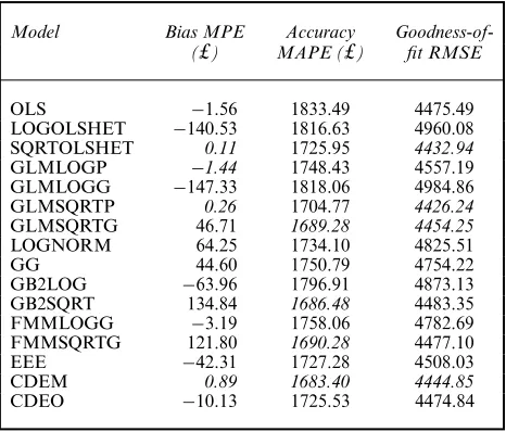
Table 5. Results of model performance, when all converged, sample size 5000, averaged across 94 replications
Model Bias MPE Accuracy Goodness-of-(£) MAPE (£) fit RMSE
OLS −1:56 1833.49 4475.49 LOGOLSHET −140:53 1816.63 4960.08 SQRTOLSHET 0.11 1725.95 4432.94
GLMLOGP −1.44 1748.43 4557.19 GLMLOGG −147.33 1818.06 4984.86 GLMSQRTP 0.26 1704.77 4426.24
GLMSQRTG 46.71 1689.28 4454.25
LOGNORM 64.25 1734.10 4825.51 GG 44.60 1750.79 4754.22 GB2LOG −63:96 1796.91 4873.13 GB2SQRT 134.84 1686.48 4483.35 FMMLOGG −3:19 1758.06 4782.69 FMMSQRTG 121.80 1690.28 4477.10 EEE −42:31 1727.28 4508.03
CDEM 0.89 1683.40 4444.85
CDEO −10:13 1725.53 4474.84
most appropriate of those featured. Interestingly, the Pearson test conducted on the estimation sample is shown here to perform well in discriminating between these competing models. This is encouraging given its ease of implementation and interpretation.
In terms of bias, models which are mean preserving in sample also perform well out of sample in these results. This is evidenced by the strong performance of OLS, GLMLOGP and GLMSQRTP, with absolute levels of mean prediction error of £1:56, £1:44 and £0:26 respectively. All models with a square-root link function underpredict costs on average, whereas some log-link function models underpredict (LOGNORM and GG) and others overpredict on average (LOGOLSHET, GLMLOGP, GB2LOG and FMMLOGG). SQRTOLSHET and CDEM perform best and third best respectively, and worst performing is GLMLOGG, which overpredicts by £147:33 on average (5.64% of the population mean).
With respect to accuracy and goodness of fit, a clear message from the results is that the best performing link function is the square-root function. The ordering of the other link functions varies. For accuracy the flexible link function of the EEE model is next best, followed by the log-link function and then OLS. For goodness of fit OLS is second best, followed by EEE whereas the log-link model is the worst. There is variation in performance among different models with the same link function, which we discuss next when considering the gains to increased flexibility. In addition, CDEM performs very well according to these criteria.
Quasi-Monte-Carlo Comparison of Parametric and Semiparametric Regression Methods 19
samples, in terms of accuracy—with FMMSQRTG the best performing model of all 16 com-pared—but the nested single-distribution case (GB2SQRTG) performs better, at all sample sizes, in terms of bias and goodness of fit (see appendix B).
Greater flexibility among the fully parametric models has an ambiguous effect on performance of forecasting means. GG is a limiting case of GB2 and its performance is better across all metrics. Conversely, LOGNORM, which is a special case of models GG and GB2, performs best of the three in terms of accuracy, the worst in terms of bias and second in terms of goodness of fit. Using GG or GB2LOG improves performance over special case GLMLOGG based on the MPE, MAPE and RMSE. Once again, the best of these four models performs worse than certain models with a square-root link function. Comparing GLMSQRTG and GB2SQRT, we can see that not much is gained from introducing more parameters, since performance is worse for GB2SQRT than for GLMSQRTG except in the cases of accuracy at sample sizes 5000 and 10000 (the difference is small at all sample sizes analysed).
Crucially, these results consider only performance based on the mean, whereas some of these models can provide information on higher moments and on other features of the conditional distribution such as tail probabilities. This is a significant qualitative advantage of parametric models over models such as linear regression, where the models have been used to predict probabilities of lying beyond a threshold value, e.g. tail probabilities; see Joneset al. (2014) who found that the GG and LOGNORM distributions perform best for the threshold values they considered. We construct graphs of bias and accuracy by decile of predicted costs. This can be thought of as analysing the fit of models for the mean of distributions of costs conditionally on observed variables, since each decile of predicted costs represents a group of observations with certain values of covariates. In previous analysis, we have considered all observations as equal, but it is possible that a policy maker prioritizes the prediction error of certain observations over others. There is considerable interest in modelling the outcomes for high cost patients, since these can be responsible for large proportions of overall costs. The highest costs are likely to be found in the highest decile of predicted costs.
Fig. 3 shows that models with the same link function follow a largely similar pattern. Those, for example, with square-root link functions underpredict in the decile of highest predicted costs, whereas log-link models overpredict in the last decile. Results with other link functions— OLS, EEE, CDEM and CDEO—all have different patterns. Generally, the first decile of predicted costs from square-root models are on average underpredictions (only GB2SQRT overpredicts in the smallest decile), which combined with the underpredicted last decile gives them a ‘u-shaped’ line. The performance of each model varies across the deciles. SQRTOL-SHET has a u-shaped line and, although it performs best in predicting costs on average across all deciles, the performance for certain groups may be worse than that of other models. For example, CDEM performs slightly worse across all 10 deciles but has a smaller range of overpredictions and underpredictions. In terms of the highest decile of predicted costs, the model with the lowest MPE is CDEO, underestimating on average £48:96. Generally this decile tends to be the largest absolute MPE for models, with values as large as an average overpredic-tion of £2211:47 in the case of GLMLOGG. Results for MAPE by decile of predicted cost are presented in the on-line appendix B, where it is striking that the pattern across all models is very similar.
A.
M.
Jones,
J.
Lomas,
P
.T
.
Moore
and
N.
Rice
(a) (b) (c) (d)
(e) (f) (g) (h)
(i) (j) (k) (l)
[image:21.485.92.640.44.420.2](m) (n) (o) (p)
Fig. 3. MPE by decile of fitted costs: (a) OLS; (b) LOGOLSHET; (c) GLMLOGP; (d) GLMLOGG; (e) EEE; (f) SQRTOLSHET; (g) GLMSQRTP;
Quasi-Monte-Car
lo
Compar
ison
of
P
ar
ametr
ic
and
Semipar
ametr
ic
Reg
ression
Methods
21
8.39
8.395 8.4 8.405 8.41 8.415 8.42 8.425
5,000 7,000 9,000 11,000 13,000 15,000 17,000 19,000 21,000 23,000 25,000
Expected LRMSE
Sample size
7.415 7.425 7.435 7.445 7.455 7.465
5,000 7,000 9,000 11,000 13,000 15,000 17,000 19,000 21,000 23,000 25,000
Expected LMAPE
Sample size
2.2 2.4 2.6 2.8 3 3.2 3.4 3.6 3.8
5,000 7,000 9,000 11,000 13,000 15,000 17,000 19,000 21,000 23,000 25,000
Expected LADMPE
Sample size
7.415 7.425 7.435 7.445 7.455 7.465
5,000 7,000 9,000 11,000 13,000 15,000 17,000 19,000 21,000 23,000 25,000
Expected LMAPE
Sample size
(a) (b)
[image:22.485.134.593.47.415.2](c) (d)
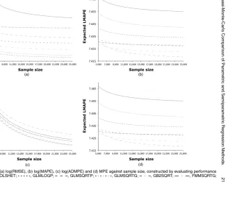
Fig. 4. Response surfaces for (a) log(RMSE), (b) log(MAPE), (c) log(ADMPE) and (d) MPE against sample size, constructed by evaluating performance on ‘validation’ set: , SQRTOLSHET;- - - - -, GLMLOGP;– – –, GLMSQRTP;----, GLMSQRTG;– –, GB2SQRT;— —, FMMSQRTG;
using the ADMPE) reduces as the sample size increases, although this happens at a similar rate across all models. Largely, though, the response surfaces for each model are parallel, indicating that the relative performance of models changes little. Further, the fact that they are flat repre-sents evidence that performance does not change for each model with increasing sample size. The exception to this is that the performance of FMMSQRTG varies with increasing sample size: its accuracy improves, and its bias worsens. This suggests that this model behaves differently with samples as small as 5000 observations, possibly because of the number of parameters that are required. On the whole, though, from samples of 5000 observations or more, there is little evidence that more flexible models require more observations than less flexible models.
7. Conclusions
We have systematically evaluated the state of the art in regression models for healthcare costs, using administrative English hospital in-patient data, employing a quasi-Monte-Carlo design to ensure rigour and drawing conclusions based on out-of-sample forecasting. We have compared recently adopted semiparametric and fully parametric regression methods that have never before been evaluated against one another, as well as comparing with regression methods that are now considered standard practice in modelling healthcare cost data.
Our results echo other studies, in that there is no single model that dominates in all respects: SQRTOLSHET is the best performing model in terms of bias and CDEM for accuracy, and in terms of goodness of fit the best performer is GLMSQRTP. This broadly corresponds to the results from the in-sample Pearson test for model selection, which highlights its potential use as a simple means to discriminate between competing models. On the basis of the Pearson test results, researchers might have implemented other power transformations of the outcome in linear regression as well as in the link functions of the GLMs. Since the EEE model estimated that the appropriate link function was somewhere between a log- and square-root function (on average 0.28 over all samples of 5000 observations), the researcher might have experimented with a cubic-or quartic-root transfcubic-ormation. However, as square-root models generally outperfcubic-ormed EEE models, there is no guarantee that results would have been better. Because there is no dominant model, the policy maker must weigh up these factors in arriving at their preferred model, based on their loss function over prediction errors. It is worth noting, however, that CDEM performs among the best four models for all three metrics. Another striking result is that four models that are commonly employed in regression methods for healthcare costs do not perform among the best four of any of the three metrics (OLS, LOGOLSHET, GLMLOGG and LOGNORM). Our analysis by decile shows the way in which models are sensitive to the choice of link function, with square-root link functions underpredicting in the decile of highest predicted costs, and log-link models overpredicting in the last decile. Finally, the response surfaces indicate that, on the whole, the more recent developments do not suffer because of the use of smaller sample sizes (from 5000 observations).
Acknowledgements
Quasi-Monte-Carlo Comparison of Parametric and Semiparametric Regression Methods 23
thank Alberto Holly, Boby Mihaylova and Sandy Tubeuf for fruitful discussions of the work. We are also grateful to John Mullahy, Will Manning, Partha Deb and Anirban Basu for their on-going support and generosity in providing feedback on our work.
References
Arrow, K. J. and Lind, R. C. (1970) Uncertainty and the evaluation of public investment decisions.Am. Econ. Rev.,60, 364–378.
Basu, A., Arondekar, B. V. and Rathouz, P. J. (2006) Scale of interest versus scale of estimation: comparing alternative estimators for the incremental costs of a comorbidity.Hlth Econ.,15, 1091–1107.
Basu, A., Manning, W. G. and Mullahy, J. (2004) Comparing alternative models: log vs Cox proportional hazard?
Hlth Econ.,13, 749–765.
Basu, A. and Rathouz, P. J. (2005) Estimating marginal and incremental effects on health outcomes using flexible link and variance function models.Biostatistics,6, 93–109.
Blough, D. K., Madden, C. W. and Hornbrook, M. C. (1999) Modeling risk using generalized linear models.
J. Hlth Econ.,18, 153–171.
Bordley, R., McDonald, J. and Mantrala, A. (1997) Something new, something old: parametric models for the size of distribution of income.J. Incm. Distribn,6, 91–103.
Buntin, M. B. and Zaslavsky, A. M. (2004) Too much ado about two-part models and transformation?: comparing methods of modeling medicare expenditures.J. Hlth Econ.,23, 525–542.
Cawley, J. and Meyerhoefer, C. (2012) The medical care costs of obesity: an instrumental variables approach.
J. Hlth Econ.,31, 219–230.
Copas, J. B. (1983) Regression, prediction and shrinkage (with discussion).J. R. Statist Soc.B,45, 311–354.
Cummins, J. D., Dionne, G., McDonald, J. B. and Pritchett, B. M. (1990) Applications of the GB2 family of distributions in modeling insurance loss processes.Insur. Math. Econ.,9, 257–272.
Deb, P. and Burgess, J. F. (2003) A quasi-experimental comparison of econometric models for health care expenditures. (Available fromhttp://econ.hunter.cuny.edu/wp-content/uploads/sites/b/ RePEc/papers/HunterEconWP212.pdf.)
Deb, P. and Trivedi, P. K. (1997) Demand for medical care by the elderly: a finite mixture approach.J. Appl. Econmetr.,12, 313–336.
Dixon, J., Smith, P., Gravelle, H., Martin, S., Bardsley, M., Rice, N., Georghiou, T., Dusheiko, M., Billings, J., Lorenzo, M. D. and Sanderson, C. (2011) A person based formula for allocating commissioning funds to general practices in England: development of a statistical model.Br. Med. J.,343, article d6608.
Duan, N. (1983) Smearing estimate: a nonparametric retransformation method.J. Am. Statist. Ass.,78, 605–610.
Duan, N., Manning, W. G., Morris, C. N. and Newhouse, J. P. (1983) A comparison of alternative models for the demand for medical care.J. Bus. Econ. Statist.,1, 115–126.
Gilleskie, D. B. and Mroz, T. A. (2004) A flexible approach for estimating the effects of covariates on health expenditures.J. Hlth Econ.,23, 391–418.
Han, A. and Hausman, J. A. (1990) Flexible parametric estimation of duration and competing risk models.
J. Appl. Econmetr.,5, 1–28.
Heckman, J. J. (2001) Micro data, heterogeneity, and the evaluation of public policy: Nobel lecture.J. Polit. Econ.,
109, 673–748.
Hill, S. C. and Miller, G. E. (2010) Health expenditure estimation and functional form: applications of the generalized gamma and extended estimating equations models.Hlth Econ.,19, 608–627.
Hoch, J. S., Briggs, A. H. and Willan, A. R. (2002) Something old, something new, something borrowed, something blue: a framework for the marriage of health econometrics and cost-effectiveness analysis.Hlth Econ.,11, 415– 430.
Holly, A. (2009) Modeling risk using fourth order pseudo maximum likelihood methods. Institute of Health Economics and Management, University of Lausanne, Lausanne.
Holly, A., Monfort, A. and Rockinger, M. (2011) Fourth order pseudo maximum likelihood methods.J. Econmetr.,
162, 278–293.
Holly, A. and Pentsak, Y. (2006) Maximum likelihood estimation of the conditional meane.y|x/for skewed dependent variables in four-parameter families of distribution.Technical Report. Institute of Health Economics and Management, University of Lausanne, Lausanne.
Huber, M., Lechner, M. and Wunsch, C. (2013) The performance of estimators based on the propensity score.
J. Econmetr.,175, 1–21.
Johnson, E., Dominici, F., Griswold, M. and Zeger, S. L. (2003) Disease cases and their medical costs attributable to smoking: an analysis of the national medical expenditure survey.J. Econmetr.,112, 135–151.
Jones, A. M. (2011) Models for health care. InOxford Handbook of Economic Forecasting(eds M. P. Clements and D. F. Hendry). Oxford: Oxford University Press.
Jones, A. M., Lomas, J. and Rice, N. (2014) Applying beta-type size distributions to healthcare cost regressions.
Jones, A. M., Lomas, J. and Rice, N. (2015) Healthcare cost regressions: going beyond the mean to estimate the full distribution.Hlth Econ., to be published, doi 10.1002/hec.3178.
Manning, W. G., Basu, A. and Mullahy, J. (2005) Generalized modeling approaches to risk adjustment of skewed outcomes data.J. Hlth Econ.,24, 465–488.
Manning, W. G., Duan, N. and Rogers, W. (1987) Monte Carlo evidence on the choice between sample selection and two-part models.J. Econmetr.,35, 59–82.
McDonald, J. B., Sorensen, J. and Turley, P. A. (2013) Skewness and kurtosis properties of income distribution models.Rev. Incm. Wlth,59, 360–374.
Mihaylova, B., Briggs, A., O’Hagan, A. and Thompson, S. G. (2011) Review of statistical methods for analysing healthcare resources and costs.Hlth Econ.,20, 897–916.
Mullahy, J. (1997) Heterogeneity, excess zeros, and the structure of count data models.J. Appl. Econmetr.,12,
337–350.
Mullahy, J. (2009) Econometric modeling of health care costs and expenditures: a survey of analytical issues and related policy considerations.Med. Care,47, suppl. 1, S104–S108.
Pentsak, Y. (2007) Addressing skewness and kurtosis in health care econometrics.PhD Thesis. University of Lausanne, Lausanne.
Vanness, D. J. and Mullahy, J. (2007) Perspectives on mean-based evaluation of health care. InThe Elgar Com-panion to Health Economics(ed. A. M. Jones). Cheltenham. Elgar.
Van de Ven, W. P. and Ellis, R. P. (2000) Risk adjustment in competitive health plan markets. InHandbook of Health Economics, vol. 1 (eds A. J. Culyer and J. P. Newhouse), ch. 14, pp. 755–845. Amsterdam: Elsevier. Veazie, P. J., Manning, W. G. and Kane, R. L. (2003) Improving risk adjustment for medicare capitated
reim-bursement using nonlinear models.Med. Care,41, 741–752.
World Health Oraganization (2007) International Statistical Classification of Diseases and Related Health Problems, 10th revision. Geneva: World Health Organization.
Supporting information