Numerical simulation of water waves in reservoirs affecting evaporation

(1)

University of Southern Queensland

Faculty of Engineering & Surveying

Numerical Simulation of Water Waves in Reservoirs

Affecting Evaporation

A dissertation submitted by

Edward Stephen Greig

in fulfilment of the requirements of

ENG4111 / ENG4112 Research Project

towards the degree of

Bachelor of Engineering (Civil)

(2)

Abstract

Predicted increases in evaporation rates from open water reservoirs will likely present

sustainability challenges for reservoir dependent communities and industries in the next

50 years. Chemical monolayers have had highly variable success in reducing

evapora-tion rates due breakup and transport by wind-wave acevapora-tion. The effect of wind-wave

stretching action on monolayers has not been quantified in the literature. The project

aim was to develop a preliminary Computational Fluid Dynamics (CFD) model to

determine the average instantaneous shear stresses under wind-wave loadings

corre-sponding to observed monolayer performance limits. Wind speeds of 0.89 m/s and 7.33

m/s are considered representative of the lower and upper limits of degraded monolayer

performance. ANSYS Fluent was used to develop a preliminary model, comprising a

horizontal tank 15 m long by 0.85 m high with water occupying the bottom half. A

constant uniform velocity wind profile was applied to the air inlet for up to five

incre-ments of the residence time of three wind speeds, 0.89 m/s, 4.11 m/s and 7.33 m/s. The

volume of fluid method was used to capture the movement of the air/water interface.

Velocity gradients were extracted from the flow fields and following a one-way analysis

of variance test, the average instantaneous shear stresses were determined to be of 0

Pa, 0.00046 Pa and 0.00058 Pa for the increasing wind speeds. These results agree with

the expectation that the instantaneous shear stress would increase with increasing wind

speed. Significant limitations for the preliminary model include insufficient run time

and a lack of average instantaneous shear stress validation. Although this study was

limited in scope, there is significant potential for model development which will assist

in understanding how monolayers are affected by wind waves, and estimating and

im-proving the operational performance of monolayers in reducing evaporation rates from

(3)

University of Southern Queensland

Faculty of Engineering and Surveying

ENG4111/2 Research Project

Limitations of Use

The Council of the University of Southern Queensland, its Faculty of Engineering and

Surveying, and the staff of the University of Southern Queensland, do not accept any

responsibility for the truth, accuracy or completeness of material contained within or

associated with this dissertation.

Persons using all or any part of this material do so at their own risk, and not at the

risk of the Council of the University of Southern Queensland, its Faculty of Engineering

and Surveying or the staff of the University of Southern Queensland.

This dissertation reports an educational exercise and has no purpose or validity beyond

this exercise. The sole purpose of the course pair entitled “Research Project” is to

contribute to the overall education within the student’s chosen degree program. This

document, the associated hardware, software, drawings, and other material set out in

the associated appendices should not be used for any other purpose: if they are so used,

it is entirely at the risk of the user.

Prof F Bullen

Dean

(4)

Certification of Dissertation

I certify that the ideas, designs and experimental work, results, analyses and conclusions

set out in this dissertation are entirely my own effort, except where otherwise indicated

and acknowledged.

I further certify that the work is original and has not been previously submitted for

assessment in any other course or institution, except where specifically stated.

0050014851

Signature

(5)

Acknowledgments

I would like to thank Dr Andrew Wandel for his supervision, patience and guidance

whilst undertaking this research project. Discussions with him were always

compre-hensive and enjoyable. His knowledge and experience in computational fluid dynamics,

statistical analysis and all matters research related was invaluable.

I would also like to thank management and my colleagues at Tumut Shire Council for

their encouragement and support.

Finally, I would like to thank my family and friends for their support, tolerance and

encouragement, without which the completion of this dissertation would not have been

possible.

This dissertation has been prepared using the USQ LaTeX template.

University of Southern Queensland

(6)

List of Figures

2.1 Amphiphilic nature of monolayers modified from Barnes (2008) . . . 11

2.2 Wave Characteristics (Dean & Dalrymple 1991) . . . 16

2.3 Volume of Fluid Method (Bakhtyar, Razmi, Barry, Yeganeh-Bakhtiary & Zou 2010) . . . 20

3.1 Computational Domain and Sampling Region . . . 24

3.2 Named Boundary Conditions . . . 27

3.3 Specific sampling points, node-averaged vs cell-centred . . . 32

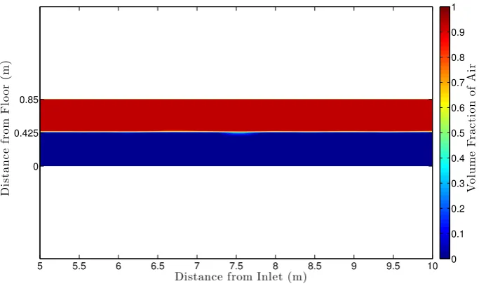
4.1 Wind Speed 7.33 m/s, Phase Plot, 10.6 s . . . 36

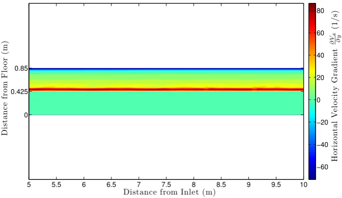
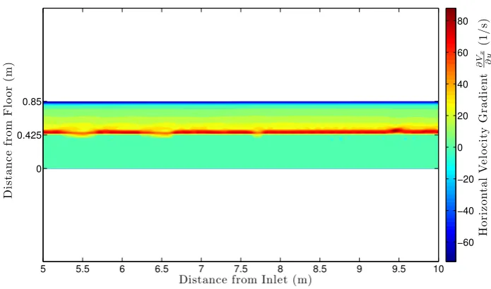
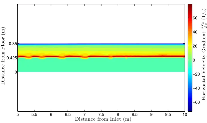
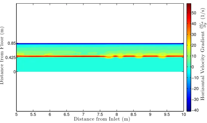
4.4 Wind Speed 7.33 m/s, Horizontal Velocity Gradient Plot, 10.6 s . . . 38

4.5 Shear stress time profiles, wind speed 7.33 m/s . . . 39

4.6 Shear stress time distributions, wind speed 7.33 m/s . . . 40

(12)

4.8 Shear Stress Sample Median vs Normalised Sampling Time . . . 41

4.9 Shear Stress Sample Standard Deviation vs Normalised Sampling Time 42 4.10 Aggregated Non-significant Shear Stress (Pa) vs Wind Speed (m/s) . . . 45

B.1 Wind Speed 7.33 m/s, Phase Plot, 2.05 s . . . 66

B.14 Wind Speed 7.33 m/s, Horizontal Velocity Gradient Plot, 2.05 s . . . 74

(13)

LIST OF FIGURES xii

C.1 Shear stress time profilea, wind speed 7.33 m/s . . . 83

D.1 Shear stress distributions, wind speed 0.89 m/s . . . 86

D.2 Shear stress time distributions, wind speed 4.11 m/s . . . 86

(14)

List of Tables

3.1 Flow variables collected . . . 23

3.2 Summary of wind speed sampling times . . . 25

3.3 Flow variables collected . . . 27

4.1 One-Way ANOVA Test Summary . . . 43

4.2 Mean Multiple Comparison Test Summary . . . 43

4.3 Kruskal-Wallis Test Summary . . . 44

4.4 Median Multiple Comparison Test Summary . . . 44

E.1 One-Way ANOVA, wind speed 0.89 m/s . . . 89

E.4 Mean Multiple Comparison Test, wind speed 0.89 m/s . . . 90

(15)

LIST OF TABLES xiv

E.8 Kruskal-Wallis Test, wind speed 4.11 m/s . . . 92

E.9 Kruskal-Wallis Test, wind speed 7.33 m/s . . . 92

E.10 Median Multiple Comparison Test, wind speed 0.89 m/s . . . 93

E.11 Median Multiple Comparison Test, wind speed 4.11 m/s . . . 93

(16)

Nomenclature

a linear wave amplitude, highest point is a crest, lowest point is a trough (m)

C= ω_k = L_T wave speed, also known as wave celerity m.s−1 η surface deviation from the mean still water level (m)

fx, fy body forces (N)

F volume fraction of a fluid phase

g gravitational acceleration m.s−2

h depth of water body (m)

H wave height, the distance between a wave crest and trough (m)

kw wave number m−1

k turbulent kinetic energy m2_.s−2

L wave length, the distance between two identical points on successive waves (m)

Ltank length of tank (m)

. λ second viscosity (Pa.s)

ν kinematic viscosity m2_.s−1

ω angular wave frequency s−1

p pressure (Pa)

(17)

Nomenclature xvi

ρ fluid density kg.m−3

t time (s)

T wave period, time between two successive crests arriving at a point (s)

u, v velocity vector components m.s−1

u0, v0 fluctuating velocity vector components m.s−1 u, v mean velocity vector components m.s−1 V two dimensional velocity vector ui+vj m.s−1

µ dynamic viscosity (Pa.s)

µT turbulent viscosity (Pa.s)

x direction of wave propagation

z= 0 still (mean) water level (x-axis)

(18)

Introduction

Predicted increases in evaporation rates from open water reservoirs in Australia will

present significant sustainability challenges in the coming years for communities and

industries which depend upon these storages. Chemical monolayers are a mitigation

technique with highly variable success in reducing evaporation rates. This variability

is primarily due to breakup and transport of the monolayer by wind-waves.

Compu-tational Fluid Dynamics (CFD) is used to investigate the average instantaneous shear

stress at the water surface resulting from wind-waves in open reservoirs corresponding

to observed monolayer performance limits. This study will complement existing

litera-ture and will assist in understanding ad improving monolayer operational performance

on open water reservoirs.

Chapter 1 provides an overview of this dissertation. The topics addressed include

back-ground, project objectives and scope, a methodology summary, project contributions

and a dissertation outline.

1.1

Background

Climate Change predictions in Australia estimate a worst case scenario increase in

average temperatures of 5◦_{C and a reduction in rainfall frequency of 50% by 2070}

(19)

1.1 Background 2

storage in open reservoirs, this may present sustainability challenges. There is a need

to minimise evaporation rates and to conserve the water already captured in reservoirs.

Numerous evaporation mitigation techniques have been investigated over the previous

decade, and earlier. These mitigation techniques included the use of wind breaks,

destratification techniques, fixed covers and chemical monolayers (Helfer et al. 2011,

McJannet et al. 2008). For all but the smallest of reservoirs, chemical monolayers are

the only approach considered to be economically feasible. This seems reasonable as the

cost of fixed structures would likely be very high and the effects of edge trees in reducing

wind action would be minimal for large reservoirs. Although evaporation reductions

in the short term may not be appreciable, over an extended term, it is suggested that

significant savings may be achieved (Palada, Schouten & Lemckert 2012).

Chemical monolayers are one molecule thick films which spread spontaneously on a

water surface and form a barrier to the passage of eater molecules from a water storage

into the atmosphere (Barnes 2008). Of the many problems with monolayers in practice,

the most significant are breakup and transport by wind and decomposition by

microor-ganisms. Breakup and transport by wind accounts for the highly variable performance

results in the literature. Waves do not necessarily break up a monolayer on their own;

however, the combination of wind and waves is believed to do this (Palada et al. 2012).

Wind and decomposition factors are extensively mentioned in the literature.

Palada et al. (2012) indicated a lack of wind-wave modelling and experimental

stud-ies in the literature concerning impacts on monolayer performance. Understanding

monolayer performance under wind-wave conditions will enable improved application

of monolayers in real-world conditions. Experimental studies by Schouten, Palada,

Lemckert, Sunartio & Solomon (2011) and Palada et al. (2012) and numerical

sim-ulations by Huang et al. (2011) using a spectral model all suggest that monolayer

performance may occur at wind speeds lower than those generally observed in field.

This seems reasonable for the Schouten et al. (2011) and Palada et al. (2012) studies

as the fetch is limited. Evidently there is a mismatch between field observations and

current laboratory trials. The spectral model used by Huang et al. (2011) suffers from

a lack of individual wave resolution. The impact of wind-waves is indicative and is

(20)

of the highest one-third of wave heights in a wave record, or four times the standard

deviation of the water surface about the mean still water level (Young 1999).

To complement these studies, CFD is proposed for modelling the average instantaneous

shear stress under wave action to quantify the breakup of monolayers. Velocity

gradi-ents can be extracted from the flow domain and used to determine the instantaneous

shear stress. Wind-waves are highly site specific and correlating shear stress to

mono-layer performance would require substantial investigation over a range of wind speeds

and surface geometries. A preliminary model is presented in this dissertation.

1.2

Project Objectives and Scope

The aim of this work was to develop a CFD model to evaluate the average instantaneous

shear stress produced under a range of wind speeds. The specific objectives of this

research project were to:

1. Research wind-wave theory and the numerical modelling of wind-waves.

2. Research evaporation of water from reservoir bodies.

3. Research the effectiveness of monolayers in reducing evaporation under the action

of wind-waves.

4. Develop a 2D / 3D Computational Fluid Dynamics (CFD) model for simulating

wave generation by wind, incorporating two phases (air/water) in a representative

reservoir.

5. Apply the developed CFD model to investigate water surface stretching in

re-sponse to wave action under defined wind loading scenarios. Validate the model

with numerical data from USQ, if available.

6. Critically analyse and discuss the surface stretching response and the implications

of wind-waves on monolayer efficiency in reducing evaporation.

7. Investigate the scale-up applicability of the wind-wave results from model output

(21)

1.3 Methodology Summary 4

8. Recommendations for further studies.

The CFD model is preliminary and it is a foundation upon which subsequent and more

complex models may be built. Time permitting, the effects of reservoir bank slope on

wind-wave heights was to be examined; this did not occur.

1.3

Methodology Summary

A review of literature was undertaken to determine the status of the numerical

mod-elling of wind-waves affecting monolayer performance in reducing evaporation. This

literature review confirmed the absence of numerical modelling of wind-waves in the

context of monolayers, with the exception of the Huang et al. (2011) paper. This

re-view provides a foundation on which to develop this project. ANSYS Fluent was used

to develop a simple multiphase model of air over water. The model was based on an

experimental wave tank used in the Schouten et al. (2011) and Palada et al. (2012)

papers. Simulations were run for the constant velocity wind speeds 7.33 m/s, 4.11 m/s

and 0.89 m/s, the limits being the observed monolayer performance range (Brink 2011).

Sampling of velocity gradients and volume fractions was conducted. This flow field data

was filtered using Microsoft Excel to identify shear stress near the water surface. The

water surface values were not used due to limitations on the accuracy of velocity

gra-dients at the interface. Matlab was used for the statistical analysis of the filtered data

and plotting purposes. Statistical tests included the One-way Analysis of Variance test

and the Kruskal-Wallis test on sample instantaneous shear stress. The effect of bank

slope on wind-wave height was not addressed in this study.

1.4

Project Contributions

The contribution of this project to the literature is the development of a simple CFD

model to examine the average instantaneous shear stress distribution of the water

sur-face for a specific water basin under three wind loading scenarios. The shear stress

(22)

included as these do not cause shear deformation of a fluid. As monolayers are a

sur-face film, this shearing stress can be used to infer the disruption of a monolayer film.

Knowledge of monolayer disruption under wind-waves will assist in improving

appli-cation of monolayers in storage reservoirs. This model is preliminary and it provides

a foundation for further development. The reporting of average instantaneous shear

stress against the limit wind speeds and recommendations for further studies indicates

that the project objectives have been satisfied.

1.5

Consequential Effects

The consequential effects of this project may be briefly considered as: ethical, safety and

sustainability issues. Ethically, this research project has been conducted in accordance

with Engineers Australia principles identified in the Code of Ethics. There is no harm

or loss to any individual person, group, or business. This research involves numerical

simulations on a computer, consequently there are no safety implications beyond that of

the author’s general health in the conducting this project. The sustainability of water

supply and agricultural industries is why this research is being undertaken and societal

benefits are mostly positive. The only negative would like be a loss of recreational use

of water reservoirs, as this would disrupt monolayers (McJannet et al. 2008).

1.6

Dissertation Outline

An overview of the chapters in this thesis is provided below.

1.6.1 Chapter 1. Introduction

Chapter 1 provides an overview of the use of monolayers for evaporation reduction in

water reservoirs. Previous studies are introduced. The project aims and a summary

methodology are provided. Project contributions are identified. A description of the

(23)

1.6 Dissertation Outline 6

1.6.2 Chapter 2. Background and Literature Review

Chapter 2 presents a review of relevant literature and selected background material

covering the topics of evaporation, monolayers, wind-waves and computational fluid

dynamics. The literature on numerical simulations of wind-waves affecting

monolay-ers is limited to a few published articles. CFD modelling of wind-waves quantifying

instantaneous shear stress at the water surface is not present in the literature.

1.6.3 Chapter 3. Methodology: Numerical Simulations

Chapter 3 presents the methodology used to investigate shear stress at the water

sur-face. A preliminary wind-wave model is developed to determine the instantaneous shear

stress at the water surface under three wind loading scenarios. Flow field velocity

gradi-ents and volume fractions were extracted. The distribution of shear stress is examined

for steady-state conditions and statistics of mean, median and standard deviation are

reported. ANSYS Fluent was used to develop a CFD model. Matlab 2010a was used

for data analysis.

1.6.4 Chapter 4. Results and Discussion

Chapter 4 presents the results of the numerical simulations. Five samples were collected

for each of the 7.33 m/s and 4.11 m/s wind speeds. Three samples were collected for

the 0.89 m/s wind speed. The distribution of samples was examined. Data Analysis

tests include One-way Analysis of Variance (ANOVA) and the Kruskal-Wallis tests.

1.6.5 Chapter 5. Conclusions and Recommendations

Chapter 5 highlights the main findings of the research, identifying the contributions of

the project to the literature. A number of recommendations for further development of

the preliminary model and for additional research on the broader subject of monolayer

(24)

1.7

Summary

Chapter 1 has provided an introduction and overview of this dissertation. The project

context, objectives and a summary methodology have been presented. An outline of

(25)

Chapter 2

Background and Literature

Review

Chapter 2 presents a review of relevant literature and background material for this

dissertation. The review appraises the current state of knowledge concerning

numer-ical simulation of monolayers under wind-wave action, specifnumer-ically shear stress at the

air/water interface, and highlights specific theoretical concepts. Surface stretching of

the water is believed to break up the monolayer coverage under wind-wave action. This

stretching, or instantaneous shear stress, is yet to be quantified in the literature.

Know-ing the shear stress correspondKnow-ing to operational limits of monolayers, over a range of

geometries , would permit estimates of monolayer performance for reservoirs.

The review of literature required accessing knowledge on a broad range of topics,

includ-ing: evaporation, monolayers, wind-wave interactions, and computational fluid

dynam-ics. A broad scope was necessary due to the complexity of the system being examined.

Many questions had to be answered, including: What are monolayers? What factors

influence their success in reducing evaporation? How do wind waves develop? How

are wind waves described, both quantitatively and qualitatively? Have any wind wave

studies concerning monolayers been completed? If so, what were the major findings?

What numerical models, if any, have been applied? Understanding aspects of each of

(26)

follow-ing chapter presents only a snapshot of the literature reviewed over the course of this

dissertation.

The literature review found that the factors influencing the success of a monolayer in

reducing evaporation are numerous, and consequently the performance of monolayers

are highly variable. Wind-waves are a major factor limiting monolayer success. Recent

experimental studies suggest that monolayers may not be successful under field

wind-wave conditions, in all but calm conditions. The review also found that only one

computational study concerning monolayers under wind wave action is reported in the

literature.

Chapter 2 is arrange thematically and covers the following topics in sequence:

evap-oration, monolayers, wind-wave studies, wind-wave theory, and computational fluid

dynamics.

Evaporation loss from dams is a significant issue in Australia, where losses up to 40% of

storage volume may be experienced (Helfer et al. 2011). CSIRO (2007) predict a

reduc-tion in rainfall intensity by up to 50% by 2070, depending upon locareduc-tion. Temperature

is predicted to increase up to 5◦_{C by 2070. For regional communities, agricultural}

and other water intensive industries, where water supply is from open reservoirs, a

reduction in the stored water may present significant sustainability challenges. Many

regional communities have had tight water restrictions in the previous decade, and this

situation will likely remain. Consequently, reducing evaporation rates in storage dams

is an important research focus.

Research centres with an interest in minimising evaporative losses in water storages

include the National Centre for Engineering Agriculture (NCEA) based at the

Univer-sity of Southern Queensland (USQ) and the now defunct Cooperative Research Centre

for Irrigation Futures (CRC). Research is also being undertaken at Griffith University

(GU).

A number of evaporation mitigation techniques to reduce evaporative loss have been

investigated in the last decade, with highly variable success being reported. Techniques

(27)

10

Of these methods, fixed covers have been most successful, with reductions up to 91%

reported when used (Helfer et al. 2011). Fixed covers provide a physical barrier which

obstructs the movement of water molecules from the water body into the atmosphere.

This easily explains why this method would be the most successful in reducing

evap-oration. Some success has been reported with wind breaks, whilst negligible results

have been found with destratification technologies (Helfer et al. 2011). Destratification

techniques focus on keeping the surface temperature cool through convection within

water bodies. A limitation of fixed covers is that they are expensive to purchase and

maintain for relatively large storages (Craig 2005). For large reservoirs, the use of

chem-ical monolayers offers a cost effective alternative. Recent research efforts concerning

reservoirs with a focus on monolayers include: the development of new monolayer

prod-ucts, the application systems, detection of monolayers on water body and wind-wave

experimentation and modelling of monolayers (Schouten et al. 2011, Brink 2011, Coop

et al. 2011, Huang et al. 2011, Palada et al. 2012).

Monolayers are artificially synthesised chemical films, one molecule thick, which

spon-taneously spread on contact with a water surface forming a effective surface barrier

(Barnes 2008). Natural monolayers may also exist at the surface of a water body;

however, the evaporation reduction potential of such monolayers is usually considered

negligible, as they lack the surface pressure to reduce evaporation loss (Hancock,

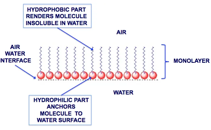
Pitt-away & Symes 2011). Artificial monolayers are amphiphilic, having both a

hydropho-bic (water repellent) and hydrophilic (water attracting) component, which forces the

monolayer to spread over the water surface. Figure 2.1 shows the amphiphilic nature of

monolayers. Under favourable conditions, such monolayers have the potential to reduce

evaporation rates up to 40% (McJannet et al. 2008). Traditional monolayers comprise

stearyl alcohol (octadecanol) and cetyl alcohol (hexadecanol) products. In the last

decade, the types of monolayers has been expanded to include prototype monolayers as

investigated by Schouten et al. (2011). Such prototype monolayers are an attempt to

overcome some of the performance issues with the octadecanol and hexadecanol type

(28)

[image:28.595.155.491.123.330.2]

Figure 2.1: Amphiphilic nature of monolayers modified from Barnes (2008)

Wide variability in the performance of monolayer performance has been reported in

field trials (Barnes 2008). A technical report by Hancock et al. (2011) indicates that

the inconsistency in the observations is a consequence of the large number of

inter-related environmental factors. This is understandable, natural systems can be highly

complex. Factors affecting the performance of monolayers include: temperature of

water, temperature of air, displacement by wind, wave field, relative humidity of air,

ground seepage, presence of a natural monolayers, incident solar radiation, biological

decomposition, surrounding terrain and the morphology of the dam. It is easily

no-ticed that many of these factors are stochastic, varying temporally. Consequently, a

deterministic solution for monolayer performance would not be easily determined. The

complexity interrelated factors would suggest that predicting monolayer performance

would be difficult. Of the number of factors influencing monolayer performance, wind

and biological decomposition are generally considered to be the most detrimental and

prevalent in the literature. Predictions of monolayer performance under winds are

mostly qualitative (Palada et al. 2012). Under conditions with little to no wind,<0.3 m/s the performance of monolayers is generally good, with 45% savings being achieved

(29)

12

spontaneously, it would make sense that the monolayer could be disturbed easily by

wind-waves.

Significant detrimental effects on monolayer performance are the result of bacterial

de-composition and break up due to wind-waves. These two factors are noticeably

promi-nent in the literature. Bacterial decomposition restricts the life of an applied monolayer

to approximately three days. For sustained evaporation resistance, a monolayer must

consequently be reapplied every few days. Application rates and locations are

impor-tant component of effective monolayer performance. Brink (2011) provides details on

the development of a universal framework for monolayer application, which provides

assistance in optimising monolayer application. Barnes (2008) states that almost all

problems with monolayer performance stem from poor resistance under wind action.

The action of wind both transports monolayer products across the water surface, and

generating waves, which are believed to act to stretch and break the up the monolayer

coverage (Schouten et al. 2011, Palada et al. 2012). As stated by Palada et al. (2012),

a quantitative assessment of wind and wave impact on monolayer performance is yet

to be substantiated in the literature. This is easily observed when reviewing the

lit-erature. The maximum wind speed for monolayers is reported as an average of 26.4

km/h (7.33 m/s) (Brink 2011).A t higher wind speeds, monolayers are considered

inef-fective. Wind induced drift of monolayers commences at approximately 3.2 km/h (0.89

m/s). Together these two limits comprise a generalised range over which monolayers

have been observed to produce a reduction in evaporation, with decreasing evaporation

resistance as wind speed increases. An understanding of wind-wave impact is necessary

for monolayer performance prediction in a reservoir.

Quantitative experimental and computational studies of wind wave affects on

mono-layer performance are noticeably lacking in the literature. Palada et al. (2012) and

Schouten et al. (2011) corroborate this observation. Observations are numerous and

are summarised by McJannet et al. (2008) and Barnes (2008). The lack of

experimen-tal studies is understandable, as wind-wave experimenexperimen-tal data is generally difficult and

costly to obtain. This data acquisition difficulty is limited by sensor technology and the

broad variability in atmospheric, water and wave fields (Sullivan & McWilliams 2010).

(30)

times required for the grid resolutions likely to be required. Quantitative experimental

studies have been undertaken by Schouten et al. (2011) and Palada et al. (2012), and a

numerical studies has been completed by Huang et al. (2011). A Computational Fluid

Dynamics (CFD) study was undertaken by Craig et a (2006); however, wind-waves

were not explicitly investigated here.

Quantitative experimental investigations of wind-wave effects on monolayer

perfor-mance have been undertaken by Schouten et al. (2011) and Palada et al. (2012). These

studies are briefly described before the limitations are presented. Both studies used

a wave tank with a wind blower and a wave paddle. The Schouten et al. (2011)

pa-per evaluated the pa-performance of six prototype monolayers against octadecanol, whilst

the Palada et al. (2012) paper only considered the octadecanol monolayer. Sinusoidal

waves with a 6 second period and 2 centimetre height were used along with wind speeds

between 0 and 5 m/s. The angle of incidence of the wind blower was varied for the

Schouten et al. (2011) paper. Whilst these studies were of a very limited scope, both

found that the octadeconal had poor evaporation resistance performance at wind speeds

greater than 1.3 m/s. The prototype monolayers generally had a higher level of

evap-oration resistance. Both papers suggested that wind waves break up and stretch out

a monolayer. Neither study included an examination of water surface shear stress in

response to wind speed.

The scope of the Schouten et al. (2011) and Palada et al. (2012) papers was limited

to several combinations of wind speeds and wave frequency. The wave amplitude was

varied in the Schouten et al. (2011) paper through the varying the angle of incidence of

the wind, which distorts the wave field. This is an attempt to produce wave field more

representative of field conditions where an irregular confused surface evolved under a

wind field. Wind waves may be considered an aggregation of many linear sinusoidal

waves, aggregating in an irregular wave field. Many combinations on wind speed and

wave amplitude would be necessary to evaluate the performance of monolayers, as

stated by Palada et al. (2012). This would be correct. A possible alternative to varying

the incidence angle, not considered in these studies, would be to vary the motion of the

wave paddle. The wave paddle could vary the wave period and amplitude through use

(31)

14

sampling would come from the distribution from a wave height time series for a specific

reservoir of interest or a reservoir with similar environmental conditions and comparable

size. In either case, the wind and waves need to be consistent with conditions that would

be observed at a dam. Another limitation is the size of the experimental equipment.

Actual dams allow waves to evolve over greater distances than can be replicated in an

experimental tank. The tank is therefore fetch limited. Larger waves of lower frequency

would seemingly have a less detrimental impact than high frequency waves. Overall,

it appears to be difficult to replicate field observations of wind-waves in a laboratory.

To complement such experimental studies, numerical simulations offer another means

of evaluating wind-wave fields.

Limitations of the Schouten et al. (2011) study included the small number of wind-wave

combinations tested and the short fetch. The Palada et al. (2012) study also has these

limitations. Huang et al. (2011) attempted to address these limitations though the

use of a numerical simulation using the spectral wave model on a full sized reservoir,

Logan’s Dam. Spectral models have been used for ocean wave forecasting by the

Bureau of Meteorology in Australia for almost 20 years (BOM 2010). The spectral

model uses a mean wind speed to evolve and transport the significant wave height

(Hs). The significant wave height is the average of the highest one-third of waves

in an observed wave field or four times the standard deviation of the surface elevation

(Young 1999). Spectral models require significantly less computational time than phase

resolving models, such as CFD, because they do not resolve individual waves. While

phase resolving models are very sensitive to initial conditions, phase averaged models

are not as individual waves are not resolved. Extensive effort has gone into refining the

spectral model over the last 20 years and the theory is well developed (Janssen 2008).

The Huang et al. (2011) study concluded that the spectral model could be used for

indicative assessment of wave field development. Whilst the significant wave height

was generally well modelled, the wave period was poor. A CFD study was undertaken

by Craig, Mossad & Hancock (2006) to develop a model for predicting evaporation

performance, however, wind waves were not investigated. No account of the water

surface stretching was considered in this study. The development of an appropriate

CFD model incorporating wind waves requires an understanding of how wind waves

(32)

measure of the distortion of the wave surface; however, as shear stress includes velocity

gradients it is arguably a better representation of surface distortion for estimating

monolayer performance.

The study of wind waves has been extensive since the Second World War, when

fore-casting sea conditions for landing operations was desired (Janssen 2008). Wind waves is

a challenging areas of study and progress has been hindered primarily due to difficulties

with capturing experimental data under field conditions (Sullivan & McWilliams 2010).

This is understandable considering the apparently complex feedback interactions

be-tween wind and waves. This limitation makes validation of wind wave models generally

difficult. Despite this limitation, significant advances in wind wave theory has

oc-curred, providing insight into how wind waves evolve and decay and facilitating the

development of wind wave models, particularly the spectral model.

Field studies of the evolution of wind-waves provides insight into how an

experimen-tal and numerical simulation model should behave. Although wind wave evolution is

complicated, the generally accepted process is described by Phillips (1957) and Miles

(1957) theories, as cited in Young (1999), as follows: as wind blows over a calm water

surface, pressure fluctuations over the surface give rise to small wavelets. As the wind

speed increases, these wavelets receive additional energy from the wind and grow

expo-nentially in height. As a wave field develops, there is shift from high frequency waves

to lower frequency waves and from a narrow spectrum to a broad spectrum of wave

heights and wavelength. Wave growth is limited by the fetch over which wind blows and

the duration of wind blowing. The shift in frequency is due to nonlinear interactions

between the waves (Janssen 2008, Mitsuyasu 2002). For enclosed basins, waves cannot

propagate away from the generating area and so are reflected either partially or fully

depending upon the basins edge geometry. The interactions would therefore be more

complicated than in a wave field where the waves may travel out of the generating area

under a wind. The extent to which reflected waves interact with a generating wave field

would depend upon the size and aspect of the water surface. From this description, it

is evident that wind waves in a water basin are a complicated phenomena. Statistical

methods have been extensively used in the literature to quantify the wind wave field,

(33)

16

H

Figure 2.2: Wave Characteristics (Dean & Dalrymple 1991)

The evolution of a wave field is a complicated process. The observed chaotic water

surface has been quantified using statistical methods. The variance of the surface

elevation about the still water level, is equated to the energy of wave field (Young 1999).

Through modelling the progress of energy using the spectral model, the wave field

properties of significant wave height are determined under a given wind field. The

spectral model assumes that waves are linear and comprises a number of finite sinusoidal

waves of variable period and wavelength. Water waves are modelled reasonably well by

linear theory (Young 1999). A simple linear wave is seen in Figure 2.2.

Equation 2.1 describes such a linear wave.

η=asin(kx−ωt) = H 2sin

2π Lx−

2π T t

(2.1)

Under linear theory, the wavelength is related to wave height through a dispersion

relationship as shown in Equation 2.2 (Young 1999):

ω2 _{= g}_k_{tanh (}_kh₎ _(2.2)

For linear wave theory to apply, the waves must be considered deep. The wavelength

relative to the water body depth must be less than 20 (Young 1999). For shallower

dams, waves are affected by the presence of the dam floor and linear theory must be

modified. Non-linear wave models account for slight raising of the wave crest and

(34)

which are computationally intensive, are not required on ocean scales for forecasting

purposes, only the general wave field conditions are approximated. Overall, the

lim-itations on experimental data acquisition and the general wave field produced by a

spectral model must be supplemented with phase resolved models, capturing the wave

field for a better understanding of monolayer behaviour under wind-waves. CFD is a

focus of wind-wave research to achieve this.

Computational fluid dynamics (CFD) involves the use of numerical algorithms to solve

the governing equations of fluid mechanics and any transport equations for additional

phenomena, for example, volume of fluid fraction. CFD studies of water waves are

reported in the literature, including Bakhtyar et al. (2010), Wang et al. (2009),Lal &

Elangovan (2008) and Lin et al. (2008) The governing equations include the

conserva-tion of mass, the conservaconserva-tion of momentum and the conservaconserva-tion of energy. Equaconserva-tions

2.3 to 2.5 are the two-dimensional governing equations for the conservation of mass and

momentum in an x-y plane (Anderson Jr 1995).

∂ρ

∂t +∇ ·(ρV) = 0 (2.3)

∂(ρu)

∂t +∇ ·(ρuV) =− ∂p ∂x+

∂τxx

∂x + ∂τyx

∂y +ρfx (2.4)

∂(ρv)

∂t +∇ ·(ρvV) =− ∂p ∂y +

∂τxy

∂x + ∂τyy

∂y ρ+fy (2.5)

The shear stresses are assumed to be equated to the velocity gradients as seen in

equations 2.6 to 2.8:

τxx =λ(∇ ·V) + 2µ

∂u

∂x (2.6)

τyy =λ(∇ ·V) + 2µ

∂u

(35)

18

τxy =τyx=µ

∂v ∂x +

∂u ∂y

(2.8)

Solution to CFD problems involves the propagation of flow field variables in temporal

and spatial domains (Tu et al. 2008). This propagation stems from an initial state.

Boundary conditions result in a deterministic solution approximating a real flow field.

For an identical model setup, boundary conditions and initial condition, CFD will

gen-erate the same solution. For turbulent flows, characterized by random fluctuations

in flow field variables, solution of the governing equations is limited by the

resolu-tion of the mesh. Very fine scales are required to capture turbulent behaviour in the

flow. Capturing such fine scales is limited by the computational power . As

com-putational capabilities presently cannot resolves all scales for turbulence, the use of

a Reynolds-averaged Navier-Stokes Equations (RANS), with an appropriate turbulent

closure model is necessary (Tu et al. 2008). Large Eddy Simulation (LES) is an another

alternative.

Present computational capabilities do not permit the governing equations of fluid

me-chanics to be solved over the full spectrum of turbulence scales for fully turbulent flows

and high Reynolds Numbers, as stated by Tu et al. (2008). Such limitations mean that

either the RANS equations are used with an appropriate turbulence closure model or

an LES model are used. RANS models have one turbulence length scale, whereas LES

models have some threshold below which the turbulence scales are not resolved. As

LES models are computationally intensive than RANS, they are not considered further

here. The RANS equations are derived from the momentum equation through use of

a mean and fluctuating velocity components. Turbulent closure models are required

to solve the additional stress terms produced by this approach. Different turbulence

models are available and each is suited to particular cases. For this study only the

two-equation k−ε closure model is used. This model was shown by Bakhtyar et al. (2010) to give reasonable results over the computational domain in their investigation

of waves breaking on a shore. Specifically, only where waves were not breaking was the

model reasonable. Using the RANS equations with k−εmodel, the turbulent shear stress are related to the velocity gradient linearly seen in Equation 2.8. The

(36)

a Newtonian fluid. This is what flow field parameter this study seeks to determine at

the water surface. Equations 2.9 to 2.11 are the two-dimensional incompressible RANS

equations discretized in an x-y plane (Tu et al. 2008). Incompressible flows have a

constant density. Body forces have been neglected in these equations.

∂u ∂x+

∂v

∂y = 0 (2.9)

∂u ∂t+

∂(uu)

∂x + ∂(vu)

∂y =−

1 ρ ∂p ∂x+2 ∂ ∂x ν∂u ∂x + ∂ ∂y ν∂u ∂y + ∂ ∂y ν∂v ∂x − "

∂ u0_u0

∂x +

∂ u0_v0 ∂y

#

(2.10)

∂v ∂t+

∂(uv)

∂x + ∂(vv)

∂y =−

1 ρ ∂p ∂y+2 ∂ ∂y ν∂v ∂y + ∂ ∂x ν∂v ∂x + ∂ ∂x ν∂u ∂y − "

∂ u0_v0

∂x +

∂ v0_v0 ∂y

#

(2.11)

The additional Reynolds stress terms are approximated as shown in equations 2.12 to

2.14. A closure model is required to use these equations.

−ρu0_u0 _{= 2}_µ

T

∂u ∂x−

2

3ρk (2.12)

−ρv0_v0_{= 2}_µ

T

∂v ∂y−

2

3ρk (2.13)

−ρu0_v0 ₌_µ

T ∂v ∂x + ∂u ∂y (2.14)

Shear stress is proportional to the velocity gradients in a Newtonian fluid. Knowing

the velocity gradients, the instantaneous shear stress can be determined. Shear stress

is highest in the boundary layers of a fluid, either where fluid is in contact with a wall

or at the interface with another fluid of significantly different viscosity. As shear stress

measurements at the water interface would be difficult to obtain experimentally, CFD is

(37)

20

interface for an appropriately discretized grid and the instantaneous shear stress at

the interface is determined. Locating the interface requires either interface-tracking or

interface-capturing methods.

Determining the instantaneous shear stress at the water surface requires knowing the

location of the water surface. Methods available to locate the water surface are either

interface-tracking or interface-capturing. Interface-tracking methods require

deforma-tion of the mesh to follow the interface. Interface-capturing methods move the interface

through a fixed computation domain, with the interface being located in cells that are

partially filled with water and air fractions. Interface-tracking methods are more

accu-rate; however, additional computational power is required and complex geometries are

limited when compared with interface-capturing methods. Interface-capturing method

have less accuracy with location of surface (Gerlach et al. 2006). Two common interface

tracking methods are Volume of Fluid (VOF) and level-set approaches. Gerlach et al.

(2006) and ANSYS (2011) compares these methods. For this study, the common VOF

approach will be used. The VOF method is limited in accuracy near the air water

in-terface because the spatial gradients of volume fraction are not continuous across cells.

This would suggest that only cells with either water or air fractions should be used

when examining velocity gradients to determine the shear stress.

The Volume of Fluid method requires transport of a scalar quantity F, the volume fraction of a cell through the computational domain. Figure 2.3 shows the volume

fraction of water in computational cells. et al.[10]measured the wave bottom boundary layer velocity in

the surf zone using particle image velocimetry and observed that a notable number of intermittent turbulent eddies penetrated into the wave bottom boundary layer. In the surf and swash zones, Sou et al.[11] investigated the velocity and turbulence fields under plunging breaking waves. Shin and Cox[12]provided a compre-hensive, accurate data set of horizontal and vertical velocities and investigated the structure of undertow, free surface, turbu-lence intensity and energy.

In order to analyze water free surface flow, it is of course impor-tant to determine the position of free surface as it varies tempo-rally. In such flows, in addition to the velocity, pressure and turbulence fields, the location of the free surface is one of the major unknowns[13]. There are two viewpoints for tracking the water free surface, namely: Lagrangian and Eulerian. In the former, water particle movement near the free surface is determined based on the local flow velocity. In the latter, the temporal variation of the free surface at a given location is computed. The Eulerian perspec-tive is more compatible with the NS equations, and is the basis of volume-of-fluid (VOF) technique [13], which will be used subsequently.

In the VOF technique[14], the volume fraction,F, of the compu-tational cell occupied by the fluid determines the free surface. The free surface is defined for cells in whichFis between zero and unity and there is at least one adjacent cell with a volume fraction of zero. The derivatives ofFcan be used to define the fluid location in any cell. From the derivatives ofF, the direction in which the variation ofFis faster is defined and hence the vector normal to the free surface. In addition, from the surface tension, the curva-ture of the free surface is defined.Fig. 1shows how VOF technique approximates the free surface.

Bradford [15] proposed a numerical solution of the NS equations in conjunction with the VOF method and investigated the applicability of different turbulence closure models for model-ing breakmodel-ing waves in the nearshore zone. Zhang and Liu[16] simulated dam break-generated bores, propagating, runup and rundown over a sloping beach. Christensen and Deigaard[17] and Christensen[18]used the NS equations in conjunction with large eddy simulation (LES) to simulate the plunging and spilling

breaking waves. A two-dimensional multi-scale turbulence model using the VOF method for modeling breaking waves was proposed by Zhao et al.[19]. These models considered single-phase water flow, not combined air and water flow.

Bakhtyar et al. [20] presented a two-dimensional numerical model for simulation of wave breaking, turbulence, undertow cur-rent and wave characteristics in the surf and swash zones. Their model is based on the Reynolds-averaged Navier–Stokes (RANS) equations, VOF and ak–eturbulence model. The model was used to investigate overturning, uprush and backwash of waves on the beach slope. Bakhtyar et al.[21–23]developed a two-phase flow model to analyze numerically sheet flow, sediment transport un-der the influence of wave breaking, and wave runup in the surf and swash zones. Their results explored different wave, beach and sediment conditions, but did not consider the effects of air entrainment during wave motion.

Entrapped air bubbles may have significant impacts on surf and swash zone hydrodynamics processes such as wave breaking, run-up/down and momentum exchange. Air–water two-phase flow is not well understood, and so there is a need for further investiga-tion into the details of this type of flow. Most previous numerical investigations focused on the water motion and neglected the ef-fect of the water–air mixing process. Air–water two-phase flow modeling has been reported in the context of coastal engineering. Hieu and Tanimoto [24] developed a two-phase flow model for simulation of wave transformations in shallow water and over a Nomenclature

d local still water depth (L)

Ei experimental values

Em experimental mean value

F fluid volume (L3_L!3₎

g magnitude of gravitational acceleration (L T!2₎

H wave height (L)

k turbulent kinetic energy (L2_T!2₎

L wavelength (L)

N number of observations

P pressure (ML!1_T!2₎

Pi predicted values

Pm predicted mean value

R2 _{coefficient of determination}

t time (T)

T wave period (T)

ui velocity component (L T!1)

u* _{shear or frictional velocity (L T}!1₎

x,z horizontal and vertical coordinates, respectively (L) Xs surf zone width (L)

Greek

h bed slope

qa air density (ML!3)

qw fluid density (ML!3)

l molecular viscosity (ML!1_T!1₎

rij strain rate tensor (L!1T!1)

! sm

ij average stress tensor (ML!2T!2)

ma kinematic viscosity of air (ML!1T!1)

mw kinematic viscosity of water (ML!1T!1)

mt eddy viscosity (L2T!1)

e turbulence dissipation rate (L2_T!3₎

j von Kármán constant

x specific dissipation rate (L2_T!3₎

f surf similarity parameter

Ck,Cx effective diffusivity ofkandx, respectively (ML!1T!1)

Dt time step (T)

rk,re,C1e,C2e,Cl empirical constants

Subscripts

b breaking point value

0.1 0.4 _0.6

1

0.7 1 1

1 1

Fig. 1.Free surface approximation using the VOF method. Left panel shows the

actual interface between the air and water phases, while the right panel represents the volume fractions associated with the interface using the VOF technique.

R. Bakhtyar et al. / Advances in Water Resources 33 (2010) 1560–1574 1561

Figure 2.3: Volume of Fluid Method (Bakhtyar et al. 2010)

The governing equations of mass and momentum are solved with a conservation

(38)

computed from Equations 2.16 and 2.17 (Gerlach et al. 2006).

∂F

∂t +∇ ·(VF) = 0 (2.15)

ρ(F) =ρwF+ρa(1−F) (2.16)

µ(F) =µwF+µa(1−F) (2.17)

Commercial and Open-Source software is available for CFD simulations, including the

Volume of Fluid approach to interface-capturing.

Commercial and open-source software is available for CFD studies. Of the software

available, only ANSYS Fluent and OpenFOAM were considered for this study. Access

to both software was available. ANSYS had a graphical user interface (GUI),

exten-sive supporting documentation and noticeable prominence in the literature reviewed.

OpenFOAM lacks a user interface and extensive documentation. A GUI and extensive

supporting documentation were the primary reasons for choosing ANSYS Fluent to

undertake CFD studies.

In chapter 2, a literature review has been undertaken, addressing the numerical

sim-ulation of monolayers under the action of wind waves. Specifically, the topic of shear

stress or surface stretching at the air water interface was reviewed. Surface stretching

of the water is believed to break up the monolayer coverage under wind wave action.

Limited experimental and numerical studies were found. These studies highlighted

that wind-wave action was a significant detriment to the performance of monolayers in

reducing evaporation rates. A single numerical simulation using a spectral model was

found to offer indicative wind-wave sizing for a water storage dam. No CFD studies

with a specific focus on wind waves water shear stresses and monolayers were found.

Using the Volume of Fluid approach, this dissertation will complement the literature in

providing additional insight into how surface stretching under generally accepted wind

(39)

Chapter 3

Methodology: Numerical

Simulations

Chapter 3 presents the methodology for undertaking a numerical simulation of a simple

reservoir to determine the average instantaneous shear stress at the water surface under

generally observed monolayer performance wind limits. Shear stress has not previously

been quantified in the literature regarding monolayer performance. It is suspected that

monolayers break up under the action of waves and wind. The evaporation resistance

of monolayers is reduced under such action. Knowledge of the average shear stress at

the observed operational limits of monolayers, for a range of surface geometries, will

permit estimation of monolayer performance in reservoirs provided the water surface

shear stresses under wind loading are known. The simple model in this project is one

of many possible geometries.

CFD is the method of choice for this study, as experimental measurement of velocity

gradients across large dams would be difficult and cost prohibitive. The purpose of

CFD is to provide insight into areas where experimentation is not easily undertaken

or the work is cost prohibitive. The distribution of water surface instantaneous shear

stresses under wind loading is one such scenario. The validation of such numerical

models is subsequently difficult. For a particular reservoir, should the shear stress of

(40)

inferred at other reservoirs. The results are specific for the geometry modelled and

subject to a number of limitations and assumptions.

Chapter 3 reviews what flow field data was collected, how the data was collected using

the software ANSYS Fluent, how the flow field data was analysed to produce

aver-age instantaneous shear stress, and provides comments on validation of the numerical

model.

3.1

Flow Field Data

This section describes what flow field data was collected and where it was collected.

Flow field data was collected at each node within the two-dimensional structured

com-putational domain with a square mesh. Table 3.1 lists the flow field data extracted

from the ANSYS Fluent model.

Table 3.1: Flow variables collected

Node Coordinates (m) Velocity (m/s) Velocity Gradients (1/s) Volume Fraction

X-coordinate Velocity magnitude Strain rate magnitude Phase 1 (air)

Y-coordinate Vx ∂Vx/∂x Phase 2 (water)

Vy ∂Vy/∂x

∂Vx/∂y

∂Vy/∂y

The variables listed in Table 3.1 were collected for the following reasons: Node

coordi-nates identify the corners of the control volume cells in the computational domain. All

flow field variables extracted from nodes are the average of the surrounding cell-centre

values. Flow velocity was extracted at each node, this was not used in analysis, but

rather was to provide a general check of velocity profiles in the domain. The strain rate

magnitude includes contributions from the normal strain rates, ∂Vy/∂y and ∂Vx/∂x.

(41)

3.1 Flow Field Data 24

determining shear stress. The shear stress or stretching rate of a fluid is proportional to

the velocity gradients,∂Vy/∂xand ∂Vy/∂x, for a Newtonian fluid. The extraction of

these velocity gradients is necessary to determine rate of shear strain and subsequently

the instantaneous shear stress. The volume fractions allow identification of the

inter-face within the computational domain. Cells with a volume fraction other than 1 or 0

contain an interface.

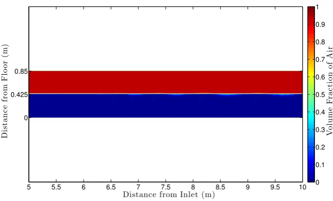
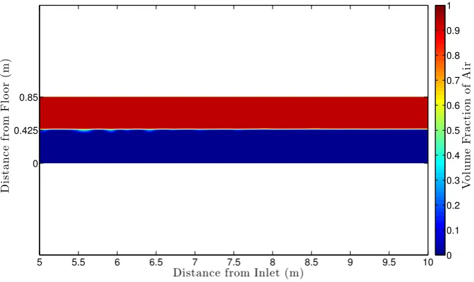
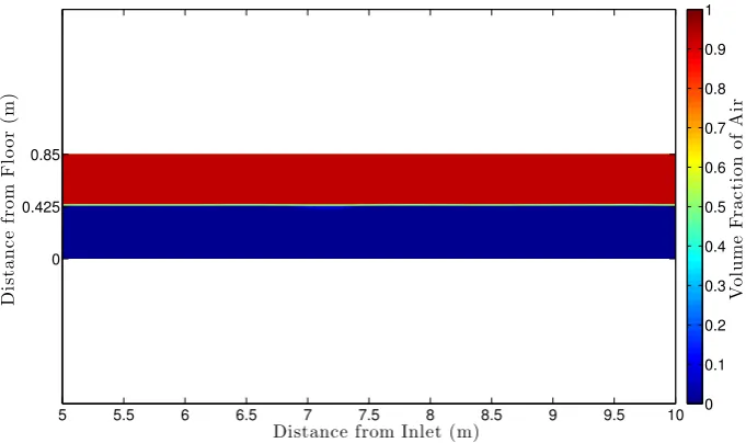
Data was collected at sample nodes within the computational domain. Figure 3.1 shows

the sampling region relative to the computational domain.

Figure 3.1: Computational Domain and Sampling Region

The sampling region from 5 to 10 m, was chosen to be 5 m away from the inlet and the

outlet of the tank to minimise the effects of the inlet and outlet boundary conditions on

the sampling region. Inspection of the phase and horizontal velocity gradient profiles,

seen in Appendix B, shows that this sampling region is acceptable and free from the

influence of the inlet and outlet boundary conditions. Waves are propagating in the

sampling region alone. Furthermore, the immediate effect of the presence end walls on

flow velocity is removed.

Flow field data was collected for three wind speeds Uinlet: 0.89 m/s, 4.11 m/s and

7.33 m/s, at intervals slightly larger than the residence times for each wind speed.

These lower and upper wind speed correspond with the observed limits for monolayer

performance (Brink 2011). Residence time is defined as the time for an air parcel to

travel from the inlet of the tank to the outlet of the tank. Residence time was calculated

(42)

divided by flow rate.

tres=Ltank/Uinlet (3.1)

The residence time intervals and sample times are summarised in Table 3.2.

Table 3.2: Summary of wind speed sampling times

Wind Speed (m/s) No. Samples Residence Time (s) Sample Times (s)

7.33 4 2.05 2.05, 4.10, 6.15, 8.20, 10.6

4.11 5 3.65 3.65, 7.31, 11.0, 14.6, 18.8

0.89 2 16.9 17.0, 34.0, 51.0

Residence time intervals for sampling were used to ensure that the data samples were

independent of each other. Specifically, one sample was collected per parcel of air

travelling from the inlet to the outlet over the duration of each consecutive residence

time. Strictly, the fluid flow samples for the water will not be independent of each other.

Waves generated over one sampling period will influence the next sampling period due

to reflection of waves from the rear tank wall and because waves are propagating slower

than air. The number of samples extracted is limited by the computational run time.

For the slower wind speeds, the residence time is substantially greater than at higher

wind speeds. The instrument for collecting the flow field data is ANSYS Fluent and it

is described in Section 3.2.

3.2

Instrument: Software ANSYS Fluent

This section describes the use of the Computational Fluid Dynamics Software ANSYS

Fluent workbench to extract the flow field data as specified in Section 3.1 of this

Chapter. Pre-processing, solving and post-processing stages are presented.

Flow field data was collected using the CFD software ANSYS Fluent Workbench. This

(43)

3.2 Instrument: Software ANSYS Fluent 26

University of Southern Queensland (USQ). ANSYS Fluent was selected in preference to

OpenFOAM due to the availability of GUI, extensive documentation and prominence

of this software in the literature. Having completed this dissertation using ANSYS

Fluent, it is now easier to understand how OpenFOAM could be used without a GUI.

Pre-processing involves defining the computational domain, subdividing the domain

into appropriate control volumes, assigning fluid properties and specifying boundary

conditions.

As seen in Figure 3.1, the two-dimensional computational domain is a 15 m long x 0.85

m high rectangle, divided into two zones of air and water, both 0.425 m high. Air is

located above the water. The domain was based on the experimental tank used in a

studies by Schouten et al. (2011) and Palada et al. (2012) with simplified boundary

conditions for the inlet and the outlet.

The simple geometry of the computational domain permits a structured square mesh

is used in preference to a unstructured mesh. This simplifies referencing of nodes and

makes post-processing of data simpler. The air and water zones were subdivided into a

relatively coarse 0.025 m square mesh. As this study is only a preliminary investigation,

a grid independence study was not undertaken. Further refinement to the mesh size

would have increased the computational run time, which was a constraint for this study.

A grid independence study is necessary though to ensure that the flow field variables

are not unduly influenced by the mesh resolution; a coarse grid is not likely to yield

sufficient accuracy. Furthermore, mesh refinement near the interface and boundaries

was not undertaken. The mesh should be refined to properly capture the velocity

gradients in the vicinity of all interfaces.

The fluid properties used in this study were the default values for air and water

avail-able in Fluent. Water default values of density and dynamic viscosity were: 998.2

kg.m−3 _{and 0.001003}_kg.m−1_s−1_{. Air default values of density and dynamic viscosity} were: 1.225kg.m−3 _{and 1.7894E-5}_kg.m−1_s−1_{. The volume of fluid method relies on} fluids being immiscible and there is no change to the relative humidity of the air and

it is unsaturated here. In a real reservoir, density and viscosity would vary as the

(44)

monolayer was not included in the model. Being one molecule thick, the grid resolution

is not fine enough to permit inclusion. Modelling may be possible should a microscopic

level be examined.

Boundary conditions are necessary to solve the governing equations of fluid dynamics

for a specified computational domain. These conditions define how a real fluid behaves

at all boundaries of the domain. Boundaries conditions are specified at the inlet and

outlet regions, all walls and the interfaces between water and air. Figure 3.2 shows the

boundary conditions used in this study.

Figure 3.2: Named Boundary Conditions

Table 3.3 presents summarises the boundary conditions used in this study.

Table 3.3: Flow variables collected

Boundary Name (m) Condition Specified

Walls Wall. No slip.

Inlet Velocity inlet. Constant uniform.

Outlet Pressure outlet.

Interface Interface.

Interior Interior.

No interaction was specified at the air/water interface; hence, no surface tension.

Fur-thermore, a mesh interface was created between the air and water. The inlet velocity

profile generated waves where the inlet contacted the water surface. Waves are also

(45)

3.2 Instrument: Software ANSYS Fluent 28

The solving stage involves specifying the flow models, initial conditions, spatial and

temporal solvers, convergence criteria, time step and iteration parameters and the

running of computations.

The Volume of Fluid and standard k−εmodels were specified. The Volume of Fluid model has two phases: air and water. The implicit body force option was specified. The

standard k−ε turbulence closure model was specified with default model constants. It was chosen as it has less equations to solve that other more complex turbulence

models and therefore less computational runtime. The key considerations here were

reduced runtime and adequacy of the model. The Reynolds stress turbulence closure

model is considered to be better for modeling swirls and rapid strain rate changes

(ANSYS 2011); however, as significant swirls are not expected in the flow, the k−ε <