C
2013. The American Astronomical Society. All rights reserved. Printed in the U.S.A.
PLANETARY CANDIDATES OBSERVED BY
KEPLER. III. ANALYSIS OF THE FIRST 16 MONTHS OF DATA
Natalie M. Batalha1,2, Jason F. Rowe3, Stephen T. Bryson2, Thomas Barclay4, Christopher J. Burke3, Douglas A. Caldwell3, Jessie L. Christiansen2, Fergal Mullally3, Susan E. Thompson3, Timothy M. Brown5,
Andrea K. Dupree6, Daniel C. Fabrycky7, Eric B. Ford8, Jonathan J. Fortney7, Ronald L. Gilliland9,
Howard Isaacson10, David W. Latham6, Geoffrey W. Marcy10, Samuel N. Quinn6,11, Darin Ragozzine6, Avi Shporer5, William J. Borucki2, David R. Ciardi12, Thomas N. Gautier III13, Michael R. Haas2, Jon M. Jenkins3, David G. Koch2,
Jack J. Lissauer2, William Rapin2, Gibor S. Basri10, Alan P. Boss14, Lars A. Buchhave15,16, Joshua A. Carter6,
David Charbonneau6, Joergen Christensen-Dalsgaard17, Bruce D. Clarke13, William D. Cochran18,
Brice-Olivier Demory19, Jean-Michel Desert6, Edna Devore20, Laurance R. Doyle20, Gilbert A. Esquerdo6,
Mark Everett21, Francois Fressin6, John C. Geary6, Forrest R. Girouard22, Alan Gould23, Jennifer R. Hall22,
Matthew J. Holman6, Andrew W. Howard10, Steve B. Howell2, Khadeejah A. Ibrahim22, Karen Kinemuchi4,
Hans Kjeldsen17, Todd C. Klaus22, Jie Li3, Philip W. Lucas24, Søren Meibom6, Robert L. Morris22, Andrej Prˇsa25,
Elisa Quintana3, Dwight T. Sanderfer22, Dimitar Sasselov6, Shawn E. Seader3, Jeffrey C. Smith3, Jason H. Steffen26,
Martin Still4, Martin C. Stumpe3, Jill C. Tarter20, Peter Tenenbaum3, Guillermo Torres6, Joseph D. Twicken3,
Kamal Uddin22, Jeffrey Van Cleve3, Lucianne Walkowicz27, and William F. Welsh28 1Department of Physics and Astronomy, San Jose State University, San Jose, CA 95192, USA;[email protected]
2NASA Ames Research Center, Moffett Field, CA 94035, USA 3SETI Institute/NASA Ames Research Center, Moffett Field, CA 94035, USA
4Bay Area Environmental Research Institute/NASA Ames Research Center, Moffett Field, CA 94035, USA 5Las Cumbres Observatory Global Telescope Network, Goleta, CA 93117, USA
6Harvard-Smithsonian Center for Astrophysics, 60 Garden Street, Cambridge, MA 02138, USA 7Department of Astronomy and Astrophysics, University of California, Santa Cruz, CA 95060, USA
8Department of Astronomy, University of Florida, Gainesville, FL 32611, USA
9Center for Exoplanets and Habitable Worlds, The Pennsylvania State University, University Park, PA 16802, USA 10Department of Astronomy, University of California Berkeley, Berkeley, CA 94720, USA
11Department of Physics and Astronomy, Georgia State University, PO Box 4106, Atlanta, GA 30302, USA 12NASA Exoplanet Science Institute/Caltech, Pasadena, CA 91125, USA
13Jet Propulsion Laboratory/California Institute of Technology, Pasadena, CA 91109, USA 14Carnegie Institution of Washington, Washington, DC 20015-1305, USA 15Niels Bohr Institute, University of Copenhagen, DK-2100 Copenhagen, Denmark
16Centre for Star and Planet Formation, Natural History Museum of Denmark, University of Copenhagen, DK-1350 Copenhagen, Denmark 17Department of Physics and Astronomy, Aarhus University, DK-8000 Aarhus C, Denmark
18McDonald Observatory, The University of Texas, Austin, TX 78712, USA
19Department of Earth, Atmospheric and Planetary Sciences, Massachusetts Institute of Technology, 77 Massachusetts Avenue, Cambridge, MA 02139, USA 20SETI Institute, Mountain View, CA 94043, USA
21National Optical Astronomy Observatory, Tucson, AZ 85719, USA
22Orbital Sciences Corporation/NASA Ames Research Center, Moffett Field, CA 94035, USA 23Lawrence Hall of Science, Berkeley, CA 94720, USA
24Centre for Astrophysics, University of Hertfordshire, College Lane, Hatfield AL10 9AB, UK 25Department of Astronomy and Astrophysics, Villanova University, Villanova, PA 19085, USA
26Fermilab Center for Particle Astrophysics, Batavia, IL 60510, USA 27Department of Astrophysical Sciences, Princeton University, Princeton, NJ 08544, USA
28Department of Astronomy, San Diego State University, San Diego, CA 92182, USA Received 2012 February 27; accepted 2012 November 14; published 2013 February 5
ABSTRACT
toward smaller planets at longer orbital periods with each new catalog release suggests that Earth-size planets in the habitable zone are forthcoming if, indeed, such planets are abundant.
Key words: catalogs – eclipses – planetary systems – space vehicles – techniques: photometric Online-only material:color figures, machine-readable tables
1. INTRODUCTION
Since initiating science operations in 2009 May,Keplerhas produced two catalogs of transiting planet candidates. The first, released in 2010 June, contains 312 candidates identified in the first 43 days ofKeplerdata (Borucki et al.2011a) and is hereafter referred to as B10. The second, released in 2011 February, is a cumulative catalog containing 1235 candidates identified in the first 13 months (Quarters 1–5)29 of data (Borucki et al.
2011b). This cumulative catalog is hereafter referred to as B11. Over 60 candidates from the B11 catalog have been confirmed, including many ofKepler’s milestone discoveries: the mission’s first rocky planet, Kepler-10b (Batalha et al. 2011); the six-transiting-planet system, Kepler-11 (Lissauer et al.2011a); the first circumbinary planet, Kepler-16ABb (Doyle et al.2011); the 2.38R⊕planet in the habitable zone (HZ), Kepler-22b (Borucki et al.2012); and the mission’s first Earth-size planets, Kepler-20 e & f (Fressin et al.2012).
In this contribution, we present new planet candidates iden-tified from the analysis of 16 months of data (Quarters 1–6). The analysis was motivated by the availability of the SOC 7.0 pipeline in the summer of 2011. A new catalog would not neces-sarily have been warranted by the addition of only one quarter of data. However, the new multi-quarter functionality ofKepler’s pipeline transit search module (Transiting Planet Search, TPS) yielded candidates that were missed in previous catalogs that used ad hoc tools for multi-quarter transit searches to detect long-period planet candidates.
We describe the results of this effort—the data (Section2), the procedures that sort transit-like signals coming out of the pipeline into viable planet candidates (Section3), and the subsequent vetting criteria that lead to increased catalog re-liability (Section 4). We describe the characterization of the planet candidates (Section 5) that begins with transit light curve modeling (Section5.1) and ultimately requires detailed knowledge of the stellar properties. An effort was made to im-prove upon the stellar properties from the Kepler Input Catalog (KIC; Brown et al.2011) by utilizing theoretical evolutionary tracks as described in Section5.2. We examine the distribu-tions of the resulting planet properties (Section 6) and take a collective look at the progress to date as we work toward the identification of Earth-size planets in the HZ. We com-pare the observed gains to those predicted by way of adding three months of data (Section7.1). The new multiple transit-ing planet systems are briefly described, as are the candidates in the HZ. Finally, in theAppendix, we provide a cumulative table of planet candidates containing the characteristics of the new candidates as well as updated characteristics of the can-didates in the B11 catalog computed using the same data used herein.
29 Quarters are defined by a requirement to roll the spacecraft 90◦about its axis to keep the solar arrays illuminated and the focal-plane radiator pointed away from the Sun. All but the first quarter are approximately 93 days in duration. In Quarter 1, the spacecraft operated in science mode for 33 days.
2. OBSERVATIONS
The data employed for transit identification were acquired between 2009 May 13 00:15 UTC and 2010 Sep 22 19:03 UTC (Q1–Q6). Over 190,000 stars were observed at some time during this period. Of these, only 127,816 were observed every single quarter. Therefore, it should not be assumed that every star tabulated herein was observed continuously for the six quarter period. While this is a reasonable assumption for the 2011 February catalog (906, or 91% of the 997 stars identified as planet hosts were observed all five quarters), it is not for the population of new candidates presented here, where only 704 (76%) of the 926 unique stars identified as planet hosts were observed all six quarters. The last column of Table3presents a string of six integers, each indicating if the target was (one) or was not (zero) observed during the quarter in question (ordered one through six, from left to right). The 4th integer (corresponding to Quarter 4) can also assume a value of 2, indicating targets located on CCD Module 3 during Quarter 4. Module 3 failed at 17:52 UTC on 2010 January 9 and never recovered. Targets located on that module were observed for a shorter time period (see below). The start and stop times for each quarter are listed in Table1. The loss of Module 3 implies that approximately 19% ofKepler’s targets will be observed three out of four quarters each year.
The data employed were taken at long-cadence (LC) whereby 270 readouts of slightly more than 6.5 second duration (6.01982 s integration and 0.51895 s read time) are co-added to 29.4 minute intervals. Quarters 1–6 yield flux time series with 1,639, 4,354, 4,370, 4,397, 4,633, and 4,397 cadences (see also Table1) corresponding to 33.5, 88.9, 89.3, 90.3, 94.7, and 89.8 days of photometry, respectively. The exception to this is the number of cadences in Quarter 4 for targets falling on CCD Module 3 (channels 5, 6, 7, and 8). Such targets were observed for 1022 cadences instead of 4397. Besides the interruption for some targets due to the Module 3 failure, each quarterly time series contains gaps, some larger than others, due to a variety of occurrences including monthly breaks for data downlink, occa-sional safe mode events, manually excluded cadences, loss of fine point, and attitude tweaks. All missing cadences are tabu-lated in the Anomaly Summary Table in Section 5 of the Data Release Notes (DRN) archived at MAST.30Also included in the DRN are the start and stop time of each quarter. This informa-tion, together with the transit ephemerides presented in Table4
is sufficient for reconstructing the number of observed transits in time series of any length.
Pixel data are converted to instrumental fluxes via Kepler pipeline software modules that calibrate pixel data (Quintana et al.2010), perform aperture photometry (Twicken et al.2010a), and correct for systematic errors (Twicken et al.2010b). The pipeline software is documented in theKepler Data Processing Handbook(KSCI-19081) at MAST. As described in Section 2 of that document, each data set is associated with a software release
30 Multi-Mission Archive at Space Telescope Science Institute;
Table 1
Data Collection Times
Quarter First Cadence Mid-time Last Cadence Mid-time Ncadence
(MJD) (UTC) (MJD) (UTC)
1 54964.011 2009 May 13 00:15 54997.481 2009 Jun 15 11:32 1639
2 55002.0175 2009 Jun 20 00:25 55090.9649 2009 Sep 16 23:09 4354
3 55092.7222 2009 Sep 18 17:19 55181.9966 2009 Dec 16 23:55 4370
4 55184.8778 2009 Dec 19 21:04 55274.7038 2010 Mar 19 16:53 4397
5 55275.9912 2010 Mar 20 23:47 55370.6600 2010 Jun 23 15:50 4633
6 55371.9473 2010 Jun 24 22:44 55461.7939 2010 Sep 22 19:03 4397
7 55462.6725 2010 Sep 23 16:08 55552.0491 2010 Dec 22 01:10 4375
8 55567.8647 2011 Jan 06 20:45 55634.8460 2011 Mar 14 20:18 3279
Notes.Quarters 1–8 are only employed in the light curve modeling used to derive the planet candidate properties. Transits are identified on a pipeline run using Quarters 1–6 only. CCD Module 3 failed in Quarter 4 on 2010 January 9 at 17:52 UTC. Targets located on Module 3 during this quarter were only observed for 1022 cadences.
Table 2
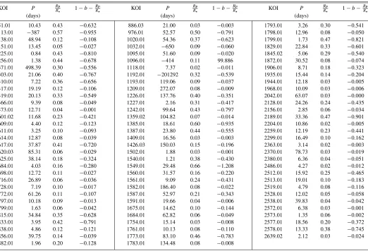
KOIs Noted as V-shaped
KOI P RP
R 1−b− RP
R KOI P
RP
R 1−b− RP
R KOI P
RP
R 1−b− RP
R
(days) (days) (days)
51.01 10.43 0.43 −0.632 886.03 21.00 0.03 −0.003 1793.01 3.26 0.30 −0.541
113.01 −387 0.57 −0.955 976.01 52.57 0.50 −0.791 1798.01 12.96 0.08 −0.050
138.01 48.94 0.12 −0.108 1020.01 54.36 0.37 −0.623 1799.01 1.73 0.47 −0.821
151.01 13.45 0.05 −0.027 1032.01 −650 0.09 −0.060 1829.01 22.84 0.33 −0.601
225.01 0.84 0.43 −0.810 1095.01 51.60 0.09 −0.020 1845.02 5.06 0.29 −0.540
256.01 1.38 0.44 −0.678 1096.01 −414 0.11 99.886 1872.01 30.52 0.08 −0.074
371.01 498.39 0.30 −0.556 1118.01 7.37 0.02 −0.011 1906.01 8.71 0.18 −0.323
403.01 21.06 0.40 −0.767 1192.01 −201292 0.32 −0.539 1935.01 15.44 0.14 −0.204
410.01 7.22 0.36 −0.656 1193.01 119.06 0.09 −0.037 1944.01 12.18 0.03 −0.005
417.01 19.19 0.12 −0.106 1209.01 272.07 0.08 −0.009 1968.01 10.09 0.03 −0.006
419.01 20.13 0.33 −0.549 1226.01 137.76 0.40 −0.351 2042.01 63.07 0.03 −0.000
466.01 9.39 0.08 −0.049 1227.01 2.16 0.31 −0.417 2128.01 24.26 0.24 −0.435
473.01 12.71 0.04 −0.001 1242.01 99.64 0.43 −0.797 2156.01 2.85 0.06 −0.034
601.02 11.68 0.23 −0.421 1359.02 104.82 0.07 −0.014 2189.01 33.36 0.47 −0.901
609.01 4.40 0.12 −0.123 1385.01 18.61 0.60 −0.935 2204.01 10.86 0.02 −0.005
611.01 3.25 0.10 −0.093 1387.01 23.80 0.44 −0.555 2259.01 12.19 0.23 −0.441
614.01 12.87 0.08 −0.039 1409.01 16.56 0.03 −0.003 2299.01 16.49 0.10 −0.162
617.01 37.87 0.41 −0.720 1426.03 150.03 0.15 −0.196 2363.01 3.14 0.02 −0.003
620.03 85.31 0.06 −0.029 1502.01 1.88 0.03 −0.001 2370.01 78.73 0.03 −0.019
625.01 38.14 0.18 −0.324 1540.01 1.21 0.38 −0.430 2380.01 6.36 0.04 −0.051
684.01 4.03 0.16 −0.280 1549.01 29.48 0.66 −1.208 2486.01 4.27 0.02 −0.012
698.01 12.72 0.11 −0.027 1560.01 31.57 0.16 −0.220 2512.01 15.92 0.25 −0.465
716.01 26.89 0.06 −0.036 1561.01 9.09 0.24 −0.431 2513.01 19.01 0.10 −0.183
728.01 7.19 0.10 −0.017 1582.01 186.40 0.08 −0.022 2519.01 4.79 0.08 −0.116
772.01 61.26 0.11 −0.107 1587.01 52.97 0.21 −0.343 2528.01 12.02 0.05 −0.058
797.01 10.18 0.09 −0.013 1591.01 19.66 0.04 −0.006 2538.01 39.83 0.04 −0.042
799.01 1.63 0.06 −0.042 1675.01 14.62 0.10 −0.144 2572.01 6.38 0.03 −0.001
815.01 34.84 0.35 −0.628 1684.01 62.82 0.06 −0.049 2573.01 1.35 0.06 −0.002
833.01 3.95 0.42 −0.791 1754.01 15.14 0.03 −0.008 2577.01 18.56 0.20 −0.372
838.01 4.86 0.12 −0.121 1761.01 10.13 0.08 −0.110 2578.01 13.33 0.38 −0.745
856.01 39.75 0.14 −0.039 1773.01 83.10 0.46 −0.783 2639.02 2.12 0.03 −0.024
882.01 1.96 0.20 −0.128 1783.01 134.48 0.08 −0.008
Notes.Negative, integer period values are intended to flag KOIs that have presented only one transit in the Q1–Q6 data. The complement of the impact parameter, b, minus the reduced planet radius,RP/R, is listed in Columns 4, 8, and 12. This diagnostic serves as an indication of a grazing, or V-shaped, transit. This value is negative if the purported planet is not fully blocking the stellar disk at mid-transit. The closer this number is to−2×(RP/R), the more severely it is grazing. Grazing transit are required to model V-shaped light curves.
number (SOC version number). For this analysis, Quarters 1–4 were processed with SOC 6.1 code, Quarter 5 was processed with SOC 6.2, and Quarter 6 was processed with a pre-release version of SOC 7.0. Specifics about the features of each can be found in the DRN at MAST that accompany each release. Note that quarterly data are reprocessed as new pipeline versions become available. Information about the data utilized herein can be found in DRN 4–9. We note that the Quarter 6 data archived
at MAST may differ slightly from the data employed here since the latter were processed with pre-release software.
3. TRANSIT IDENTIFICATION
[image:3.612.46.568.253.609.2]Table 3
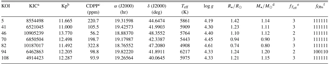
Host Star Characteristics
KOI KICa Kpb CDPPc α(J2000) δ(J2000) Teff logg R/R M/Md fTeff
e fObsf
(ppm) (hr) (deg) (K)
5 8554498 11.665 220.7 19.31598 44.6474 5861 4.19 1.42 1.14 3 111111
41 6521045 11.000 105.5 19.42573 41.9903 5909 4.30 1.23 1.11 3 111111
46 10905239 13.770 56.2 18.88370 48.3552 5764 4.40 1.10 1.12 2 111111
70 6850504 12.498 198.7 19.17987 42.3387 5443 4.45 0.94 0.90 3 111111
82 10187017 11.492 322.8 18.76552 47.2080 4908 4.61 0.74 0.80 3 111111
94 6462863 12.205 98.8 19.82220 41.8911 6217 4.33 1.24 1.20 2 100110
108 4914423 12.287 93.9 19.26564 40.0645 5975 4.33 1.21 1.15 3 111111
Notes.
aKepler Input Catalog number.
bApparent magnitude in theKeplerbandpass.
crms of Combined Differential Photometric Precision from Quarters 1–6 in units of parts per million. dStellar Mass is derived from surface gravity and stellar radius.
eFlag indicates source ofTeff, logg, andR
as follows: (0) derived using KICJ−Kcolor and linear interpolation of luminosity class V stellar properties of Schmidt-Kaler (1982); (1) KICTeffand loggare used as input values for a parameter search of Yonsei–Yale evolutionary models yielding updatedTeff, logg, andR; (2)Teff, logg, andRare derived using SPC spectral synthesis and interpolation of the Yale–Yonsei evolutionary tracks; (3)Teff, logg, andRare derived using SME spectral synthesis and interpolation of the Yale–Yonsei evolutionary tracks.
fConcatenation of six integers, one for each of the six quarters of spacecraft data; the value of each successive integer indicates whether or not the star was observed for each of the successive quarters; a zero indicates the star was not observed that quarter; one indicates the star was observed the entire quarter; two indicates the star was observed only part of the quarter (relevant for stars on CCD Module 3 in Quarter 4); for example, a value of 000111 indicates the star was observed in Quarters 4, 5, and 6 but not in Quarters 1, 2, or 3.
(This table is available in its entirety in a machine-readable form in the online journal. A portion is shown here for guidance regarding its form and content.)
Table 4
Planet Candidate Characteristics: Light Curve Modeling
KOI tdur Depth S/Na T0b σT0 Periodb σP d/Rc σd/R RP/R σRP/R b
d σ
b χ2
(hr) (ppm) (days) (days) (days) (days)
5.02 3.6882 20 8.5 66.36690 0.01456 7.0518564 0.0002848 9.797375 0.558680 0.00428 0.00038 0.74970 0.29480 1.4 41.02 4.4764 76 36.8 66.17580 0.00321 6.8870994 0.0000617 6.177925 0.120880 0.00918 0.00016 0.86500 0.10100 1.2 41.03 6.1426 92 23.2 86.98394 0.00667 35.3331429 0.0006257 18.376942 0.359570 0.01042 0.00030 0.92010 0.09750 1.2 46.02 3.7909 58 9.7 65.51465 0.01139 6.0290779 0.0001918 6.892009 0.118930 0.00799 0.00059 0.83650 0.22630 1.2 70.05 3.6029 99 18.4 68.20094 0.00566 19.5778928 0.0002980 28.131385 3.635640 0.00998 0.00039 0.74920 0.23260 1.1
. . . . . . . . . . . . . . . . . . . . . . . . . . . . . . . . . . . . . . . . . . . . .
1612.01 1.2288 30 12.2 65.68197 0.00209 2.4649988 0.0000198 11.917724 4.152810 0.00531 0.00025 0.63910 0.50290 1.3 1613.01 4.2342 78 22.0 74.08600 0.00466 15.8662120 0.0001989 18.014821 4.615850 0.00933 0.00064 0.78970 0.35850 1.0 1615.01 1.7195 108 31.9 65.23335 0.00161 1.3406380 0.0000107 4.967419 1.056310 0.00961 0.00024 0.58290 0.28050 1.6 1616.01 2.4240 147 23.0 72.41072 0.00363 13.9328148 0.0001269 41.632554 20.251940 0.01117 0.00119 0.35180 0.91970 1.2 1618.01 3.5409 29 19.0 65.25658 0.00455 2.3643203 0.0000365 3.150859 0.318180 0.00547 0.00020 0.81200 0.17720 1.2
Notes.Invalid and/or missing data are given values of−99. Zero denotes a value smaller than the recorded precision. aS/N of the phase-folded transit signal computed from modeling of Quarters 1–8 data.
bBased on a linear fit to all observed transits. Periods estimated from the duration of a single transit and knowledge of the stellar radius are rounded to the nearest integer and multiplied by−1.
cTo first order, this parameter is equivalent to the ratio of the planet–star separation (at the time of transit) to the stellar radius. In the case of a zero-eccentricity orbit, it is equivalent to the reduced semimajor axis,a/R.
dNote that there is a strong covariance betweenbandd/R .
(This table is available in its entirety in a machine-readable form in the online journal. A portion is shown here for guidance regarding its form and content.)
is described in Jenkins et al. (2010b), Tenenbaum et al. (2012), and in theKepler Data Processing Handbookat MAST. Be-fore searching for transits, the software stitches together each quarterly data segment to form one contiguous light curve. To accomplish this, TPS removes a polynomial fit constrained to achieve zero offset and zero slope in the first and last day of each quarter and to ensure that the result is approximately zero-mean and wide sense stationary. TPS then identifies and removes strong sinusoidal features from quarterly light curves via a periodogram-based approach. Finally, the gaps between quarters are filled via an autoregressive modeling technique to condition the time series for the Fast-Fourier-Transform-based detection algorithm.
[image:4.612.41.578.357.499.2]Table 5
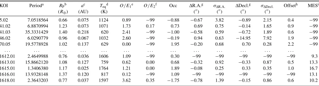
Planet Candidate Characteristics and Vetting Metrics
KOI Perioda RPb ac Teqd O/E
1e O/E2f Occ ΔR.A.g σΔR.A. ΔDecl.g σΔDecl. Offseth MESi
(R⊕) (AU) (K) () () () ()
5.02 7.0518564 0.66 0.075 1124 0.89 −99 −0.88 −0.67 3.82 −0.89 2.15 0.4 −99
41.02 6.8870994 1.23 0.073 1071 1.73 0.17 0.73 0.69 0.75 −0.14 1.65 0.9 −99
41.03 35.3331429 1.40 0.218 620 2.41 −99 −1.00 −0.58 0.59 −0.72 1.89 0.6 −99
46.02 6.0290779 0.96 0.067 1032 2.60 −99 −0.19 0.94 0.63 −14.95 7.92 1.9 −99
70.05 19.5778928 1.02 0.137 629 0.00 −99 1.95 −0.20 0.68 0.70 0.28 2.2 −99
. . . . . . . . . . . . . . . . . . . . . . . . . . . . . . . . . . . . . . .
1612.01 2.4649988 0.76 0.036 1606 1.09 −99 0.30 −99 −99 −99 −99 −99 9.3
1613.01 15.8662120 1.08 0.127 759 0.62 0.00 0.68 −0.32 0.92 −0.33 0.87 0.5 13.3
1615.01 1.3406380 1.17 0.025 1764 1.21 0.00 1.89 −0.08 0.25 0.33 0.35 1.0 16.7
1616.01 13.9328148 1.37 0.120 817 0.12 −99 1.09 −99 −99 −99 −99 −99 13.1
1618.01 2.3643203 0.77 0.037 1597 3.62 0.35 −1.75 −0.78 1.39 −0.15 0.86 0.6 10.2
Notes.Invalid and/or missing data are given values of−99. Zero denotes a value smaller than the recorded precision.
aBased on a linear fit to all observed transits. For candidates with only one observed transit, the period is estimated from the duration and knowledge of the stellar radius; values are then rounded to the nearest integer and multiplied by−1.
bProduct ofr/R∗and the stellar radius given in Table1.
cBased on Newton’s generalization of Kepler’s third law and the stellar mass in Table3. dSee the main text for discussion.
eOdd/even statistic derived from light curve modeling. fOdd/even statistic reported by Data Validation pipeline. gOffset is transit source position minus target star position. hDistance to source position divided by noise.
iReported by the pre-release SOC 7.0 TPS pipeline run on Q1–Q6 data; MES is the detection statistic akin to a total S/N of the phase-folded transit but constructed using the matched filter correlation statistics over phase and period.
(This table is available in its entirety in a machine-readable form in the online journal. A portion is shown here for guidance regarding its form and content.)
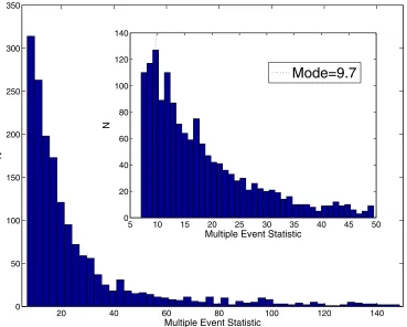
identify threshold crossing events (TCEs): instances where a given period and epoch exceed the detection threshold of 7.1σ. Fourteen distinct transit searches are conducted, each using a different pulse duration (1.5, 2.0, 2.5, 3.0, 3.5, 4.5, 5.0, 6.0, 7.5, 9.0, 10.5, 12.0, 12.5, and 15 hr) as described in Jenkins et al. (2010b) and Tenenbaum et al. (2012). The maximum multiple event statistic (MES) over all durations is an estimate of the ratio of the transit depth to the uncertainty in the transit depth as a fitted parameter for the given rectangular transit pulse train at which the maximum occurred. At a threshold of 7.1σ, fewer than one false alarm is expected over the baseline mission duration due to statistical fluctuations. This defines the threshold for consideration as a viable candidate. Often, several of the matched filter pulse durations yield a detection statistic that passes our criterion (as expected), in which case the highest value is adopted. MES values are presented in Column 14 of Table5. Two hundred ninety-one candidates are assigned MES values of−99 signifying an invalid value. This occurs when the period returned by the pipeline is not the final period derived from full light curve modeling.31 MES values of −99 also occur for the new “multis” (additional candidates associated with stars already having at least one candidates) identified by non-pipeline products (see below).
The analysis presented here stems from a TPS run used for verification and validation of the pre-release SOC 7.0 pipeline. It was the first time that TPS was run using the multi-quarter functionality. Such functionality was not available for the production of the B11 catalog. Long-period candidates in the B11 catalog were identified using a box least-squares (BLS) algorithm (see, for example, Kov´acs et al. 2002). The BLS frequency spectrum is normalized by a smoothed time-series
31 TPS usually gets the correct period for single transit signatures but occasionally chooses a multiple of the true period as the maximum, and is sometimes confused by light curves with multiple transiting planet signatures.
periodogram in order to remove the 1/f noise floor which can dominate the detection statistic when searching for long-period events.
TPS returned 104,999 unique targets with at least one se-quence of periodic transits yielding MES> 7.1 (i.e., TCEs). The majority of these TCEs are triggered by transients in the normalized light curves. Hence, the list is further culled by ap-plying a second criterion based on the ratio of the MES to the maximum single event statistic (SES) contributing to the MES. The SES is the maximum correlation statistic in the time domain at a given test period. MES/SES should be comparable to the square-root of the number of observed transits. Tenenbaum et al. (2012) shows that there are two distinct populations of TCEs, with a dividing line at MES/SES=√2. Below this value, detec-tions are likely the result of two highly unequal single events as opposed to two legitimate transits of equal depth and duration. Discarding TCEs with MES/SES<√2 reduces the number of viable TCEs from 104,999 to 4531.
the KOI number to distinguish between multiple candidates as-sociated with the same star. They are assigned in the order they were identified.
Future pipeline runs include improvements that increase the detection efficiency of multiple planet systems thereby eliminating the need to run offline tools and increasing sample uniformity.
4. CANDIDATE VETTING
The procedures described in Section3 produce 1390 KOIs that are then vetted for astrophysical false positives in the form of eclipsing stellar systems. Here, we describe the suite of statistical tests employed. They are separated by the type of data they operate on. Statistical tests derived from the flux time series and the corresponding transit models are described in Section4.1, while statistical tests derived from pixel-level data are described in Section4.2. Both make use of pipeline products as well as offline analyses. The pipeline module that evaluates KOIs for likely false positives, referred to as Data Validation (DV), is described by Wu et al. (2010) and the Kepler Processing Handbookat MAST. Section4.3describes the overall procedures that were followed to promote a KOI to planet candidate status.
As work to identify and vet candidates progressed, new products became available. Quarter 7 and Quarter 8 photometry, for example, was available in the summer of 2011. These data were utilized in the offline (i.e., non-pipeline) light curve modeling used to determine various vetting metrics, as well as the properties of the planet candidates tabulated in Tables4and5
and described Section5.1. Moreover, testing of pre-release SOC 8.0 code (also using Q1–Q8 data) in the fall of 2011 produced significantly improved DV reports and metrics and were also used to vet the Q1–Q6 candidates reported in this contribution. A subset of the vetting metrics used for candidate evaluation are provided in Table5so that users can identify the weaker candidates and know what types of problems to look for. These metrics are described in turn below and summarized in Section4.3.
4.1. Tests on the Flux Time Series
For each KOI, the even-numbered transits and odd-numbered transits are modeled independently using the techniques de-scribed in Section 3. The depth of the phase-folded, even-numbered transits is compared to that of the odd-even-numbered transits as described in Batalha et al. (2010a) and Wu et al. (2010). A statistically significant difference in the transit depths is an indication of a diluted or grazing eclipsing binary system. A similar metric is computed by the DV pipeline module as de-scribed by Wu et al. (2010). Each uses a different methodology for detrending the light curves (i.e., filtering out stellar vari-ability), and both proved useful and are tabulated in Columns 6 (modeling-derived statistic:O/E1) and 7 (DV-derived statistic: O/E2) of Table5. In general, 3σwas the threshold for flagging a KOI as a false positive. However, when the two values disagreed, we deferred to the DV statistic owing to its more sophisticated whitening filters. One hundred forty-three KOIs in Table5have O/E1 >3 while only seven haveO/E2 > 3. Five have both O/E1 andO/E2 larger than 3σ but are otherwise clean can-didates. Further inspection of their light curves suggested that stellar variability and/or instrumental transients were driving an anomalously high odd/even statistic, and the candidates were retained. In 121 cases, the DV model fitter failed, thereby pre-cluding quantification of an odd/even statistic. In 18 of these
cases,O/E1 is larger than 3σ and the candidate was retained anyway. While most of these are marginal cases near the 3σ cutoff, users are cautioned that exceptions exist and should be examined independently on a case-by-case basis.
The modeling allows for the presence of a secondary eclipse (or occultation event) near phase=0.5 as a means of identi-fying diluted or grazing eclipsing star systems. The Secondary Statistic (Column 8 of Table5) is the relative flux level at phase 0.5, divided by the noise. As such, it can have positive as well as negative values. While its presence does not rule out the plane-tary interpretation, it acts as a flag for further investigation. More specifically, the flux decrease is translated into a surface temper-ature assuming a thermally radiating disk, and this tempertemper-ature is compared to the equilibrium temperature of a low-albedo (0.1) planet at the modeled distance from the parent star. If the flux change is not severe enough to rule out the planetary in-terpretation (ascertained by the difference between the surface temperature and equilibrium temperature), the candidate is re-tained. Eight KOIs retained in the catalog have a statistic outside of (negative) 3σ. In each of these cases, it appears possible that the occultation signal is a result of stellar and/or instrumental flux changes. This statistic is relevant primarily for short-period orbits where circularization is expected since the search is only done at phase 0.5. The DV pipeline module checks to see if additional transit sequences were identified in the light curve at the same period but different phase. No such sequences were identified for the candidates reported here.
Table 2 lists KOIs (both old and new) that are V-shaped. The shape of a transit is not used as a diagnostic for rejecting planet candidates. The right combination of properties and geometry can, indeed, produce ingress and egress times that are a significant fraction of the total transit duration (e.g., grazing transits). However, a diluted eclipsing binary system is another possible interpretation and does not require such a narrow range of inclination angles (impact parameters). The false-positive rate amongst theV-shaped candidates is expected to be higher than the false-positive rate of the general population. A metric is constructed to flag such cases: 1−b−(RP/R). The objective is to alert the reader to populations with larger false-positive rates and also to avoid classification of a transit as V-shaped because of smear produced by the 30 minute cadence. Errors in the metric are dominated by the uncertainty of the modeled impact parameter which can be quite high. Therefore, all flagged light curves were visually inspected.
Negative values imply that the purported planet is not fully covering the stellar disk at mid-transit. The closer the metric is to−2×(RP/R), the more severely it is grazing. A grazing geometry is required to model V-shaped transits that are not caused by a large planet-to-star size ratio. The KOIs with light curves modeled as grazing transits are listed in Table2together with the orbital period and reduced radius.
4.2. Tests on the Pixel Data
−5 0 5 −5
0 5
15095972, 18.041 12505654, 14.988
← E (arcsec)
N (arcsec)
→
−5 0 5
−5 0 5
15095972, 18.041 12505654, 14.988
← E (arcsec)
N (arcsec)
[image:7.612.52.561.59.273.2]→
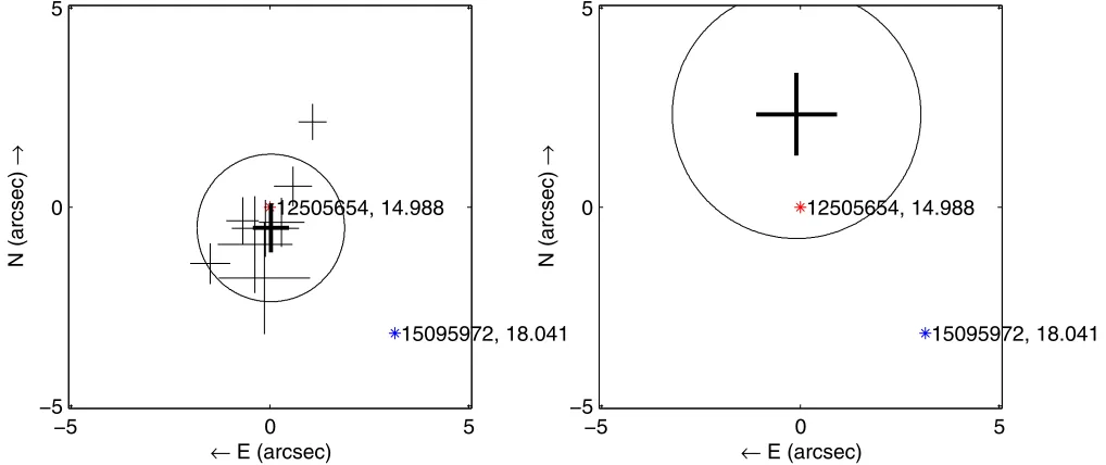
Figure 1.Transit source location determined by the difference image (left panel) and photo-center motion (right panel) techniques for KOI-2353. On the left, the thin crosses show the individual quarter measurements, and the bold cross shows the multi-quarter average. On the right, the transit location inferred from the multi-quarter joint fit to the photo-center motion is shown. In both panels the length of the cross arms show the 1σuncertainties in R.A. (x-axis) and decl. (y-axis). The circle shows the 3σuncertainty in the offset distance. The asterisks show star locations, labeled by Kepler ID and Kepler magnitude, with the centered asterisk showing the location of the target star. This is a clear example where the transits are associated with the target, rather than the nearby, faint background star.
(A color version of this figure is available in the online journal.)
Photo-center motion is measured by computing the flux-weighted centroid of all pixels downlinked for a given star both in and out of transit. Fluxes associated with a transit event are identified using the ephemerides and transit durations listed in Table2. The flux-weighted centroids are calculated in one of two ways. KOIs that were processed with the DV module in the SOC pipeline have a flux-weighted centroid measurement for every cadence. The in versus out of transit centroid offset is computed by performing a least-squares fit of the pipeline-generated transit model to the multi-quarter centroid time series, the idea being that the behavior of the flux-weighted centroid time series will mirror that of the flux time series. The centroid offset is the amplitude of the “transit” pulse in the model fit.
KOIs that were not processed by the DV pipeline module are treated slightly differently in that the flux-weighted centroid is computed for a pixel image constructed by taking the average of images in a single quarter when the KOI is not transiting. It is then compared to the flux-weighted centroid for a pixel image that is the average of images in the same quarter when the KOI is transiting. The centroid offset is the difference between the in and out of transit centroids. Quarterly offsets are averaged together as described below. Once the centroid offset is computed, the source location is inferred by scaling it by the inverse of the flux as described in Jenkins et al. (2010a). Difference image analysis takes the difference between av-erage in-transit pixel images and avav-erage out-of-transit images. Barring pixel-level systematics and field-star variability, the pix-els with the highest flux in the difference image form a star image at the location of the transiting object, with flux level equal to the fractional depth of the transit times the original flux of the star. Performing a fit of theKeplerpixel response function (PRF; Bryson et al.2010) to both the average difference and out-of-transit images gives the sky location of the out-of-transit source and the target star. The offset of the transit source from the target star is then defined as the transit source minus target star location. For most KOIs, the difference image offset is computed per quarter, and the quarterly offsets are averaged as described below. For a
small number of KOIs with very low signal-to-noise ratio (S/N), a computationally expensive joint multi-quarter fit is performed, with uncertainties estimated via a bootstrap analysis.
In principle, both the photo-center motion and difference image techniques are similarly accurate for isolated stars and sufficiently high S/N transits, but the techniques have different responses to systematic error sources such as field crowding. The photo-center method is more sensitive to noise for low-S/N transits and crowding by field stars. In particular, the estimate of the transit source location by scaling the offset is highly sensitive to incompletely captured flux for either the target star or field stars in the aperture.
In the difference image method, the PRF fit to the difference and out-of-transit pixel images is biased by PRF errors described in Bryson et al. (2010), as well as errors due to crowding. Defining the centroid offset as the difference between the out-of-transit and difference images nearly cancels the PRF bias because both fits are subject to the same error. Bias due to crowding, however, is more of an issue. Excepting cases in which background stars are strongly varying, a difference image removes most point sources, leaving the transit signal as the predominant change in flux. The average out-of-transit image, on the other hand, contains all point sources. Consequently, the offset (formed by comparing a direct image and a difference image) may contain a bias.
This method is less effective in reducing the centroid bias for long-period candidates. In particular, single-transit candidates that appear in only one quarter may have unknown biases in their centroid positions that are not accounted for in the centroid uncertainties.
The above centroid analysis was performed using data from Quarters 1–8. The transit source location offsets reported in Table5are from the difference image method since it is more reliable as evidenced by consistently smaller uncertainties com-pared to the photo-center motion method. A candidate passes the photo-center vetting step when its multi-quarter transit source offset is less than 3σ. There are, however, exceptions. KOIs having transit source offsets larger than 3σ were identified as having systematic errors (e.g., crowding biases) that are likely causing the large apparent offset. Modeling efforts to confirm these systematics are currently underway.
In some cases, the PRF fit algorithm failed, typically due to low quarterly S/N or to bright field stars that prevented reliable determination of the target star location via PRF fit. We retain these targets when visual inspection of the difference image indicates that the change in flux due to the transit is on the target star. Finally, difference imaging is very inaccurate for saturated targets, and we retain saturated candidates for which the difference images show no obvious indication of a background source. Offset values for slightly saturated stars (Kp between 10.5 and 11.5) are likely accurate to within 4 (one pixel), while offset values for highly saturated stars (Kp<10.5) should be disregarded. Transit source offset values are set to−99 when we feel that the centroid measurement is unreliable.
4.3. Promotion to Planet Candidate
KOIs were divided amongst more than 20 science team members for evaluation of the following metrics: (1) odd/even statistic, (2) occultation test, (3) quality of model fit, (4) long/short period comparison, (5) single-quarter photo-center motion, and (6) multi-quarter photo-photo-center motion. An integer value of 0, 1, or 2 was assigned to each metric to indi-cate if the test clearly passed (0), was ambiguous (1), or clearly failed (2). A similar flag was ascribed to the visual appear-ance, where examples of suspicious characteristics would in-clude markedly V-shaped transits, red noise and/or outliers in the time series calling into question the reliability of the tran-sit signal, anomalously long trantran-sit durations, poor light curve fits, obvious secondaries, etc. Each candidate was then desig-nated “yes,” “no,” or “maybe.” Candidates flagged as ambiguous (maybe) were re-evaluated. In most cases, this required updated light-curve modeling, more detailed inspection of the software pipeline products, and/or further scrutiny of the pixel flux anal-ysis yielding photo-center statistics.
Once every KOI was assigned a “yes” or “no” designation, the integer flags were summed and the distribution for the two populations was compared. This elucidated a small number (<10) of inconsistencies in which flags indicate a problem yet the KOI was assigned a “yes” designation. These were independently evaluated.
The period and location on the sky of every new KOI was cross-checked against the list of previously known KOIs and the catalog of eclipsing binaries (Prˇsa et al. 2011; Slawson et al. 2011). This is a safeguard against redundancy. More importantly, though, the cross-check serves to identify flux contamination from bright eclipsing binaries that the photo-center analysis missed. Approximately 25 targets within 20of
an existing KOI or eclipsing binary with commensurate (within a factor of 1, 2, 3) orbital period (to within 5 minutes) were identified. In this manner, we also identified two small swarms of spatially co-located stars, each with a transit-like event at a commensurate orbital period. The lack of sizable photo-center motion and the spatial extent of the contaminating flux suggests that scattered light (e.g., an optical ghost from a bright eclipsing binary at the focal plane anti-podal position) is responsible.
Every one of the 1 390 KOIs evaluated here will appear either in this contribution as a viable planet candidates, or in the associated false-positive catalog (S. Bryson et al. 2012, in preparation), or in future versions of the Eclipsing Binary Catalog.
Eight high-S/N (>30σ) single transit events were identified and included in the catalog. Their corresponding orbital periods are estimated from the transit duration and knowledge of the stellar radius assuming zero eccentricity. The periods are then rounded to the nearest integer and multiplied by −1 so as to distinguish them from the candidates that have reliable orbital ephemerides. Parameters requiring an accurate period (e.g., odd/even statistic, semimajor axis, etc.) are set to−99, which is the value adopted globally for unreliable, spurious, or unknown values.
The final list of viable planet candidates is presented in Table4with additional information listed in Table5. In addition to the MES from the Q1–Q6 TPS run, the following vetting metrics are provided: (1) the odd/even statistic that tests for an eclipsing star system of nearly equal-mass components at twice the period (Columns 6 and 7), (2) the occultation (secondary) statistic that tests for a weak secondary event inconsistent with a planet occultation at phase 0.5 (Column 8), (3) the photo-center offsets in R.A. and decl. measured in arcsec and their associated uncertainties (Columns 9–12), and (4) the total photo-center offset position measured in units of the noise (Column 13).
Analysis is based on a blend of both quantitative metrics and manual inspection. Both the promotion from TCEs to KOIs and the promotion of KOIs to planet candidates has a human element that not only increases the reliability of the catalog but also reduces the number of false negatives that are discarded. The reader is cautioned, however, that reliability and efficiency of human scrutiny is difficult to quantify. Consequently, sample statistics derived from this sample will be difficult to interpret. This will improve with each subsequent catalog release as we work toward automation and uniformity of procedures and metrics.
5. PROPERTIES OF PLANET CANDIDATES
Here, we describe the light curve modeling that characterizes both the orbital and physical characteristics of each planet candidate.
5.1. Model Fitting
of the companion is much less than the mass of the central star. For a Jupiter-mass companion, an error of 0.02% will be incurred on the measurement ofρ, a 0.1Mcompanion would skew our estimate ofρby approximately 2%, and a 0.5 M companion would induce a systematic error of 41% onρ. These assumptions give
a R
3 π
3GP2 =
(M+Mp) 4π
3R3
≈ M 4π
3R3
=ρ, (1)
wherea/Ris referred to as the reduced semimajor axis. Transits probe a small portion of an orbit giving little or no information about eccentricity. We assume circular orbits in our models. Consequently, the reduced semimajor returned by light curve modeling does not necessarily yield an accurate determination of the semimajor axis nor the stellar density. To emphasize this point, we purposely report the parameter asd/Rwhich, to first order, is equivalent to the ratio of the planet–star separation during transit to the stellar radius. It is equivalent toa/R for zero-eccentricity orbits.
A full orbital solution is required to correctly determine stellar parameters from transit modeling. Great care must be taken when interpreting the fitted stellar parameters. A mismatch between the reported stellar parameters and a transit-derived stellar parameter can be interpreted as evidence of: an eccentric orbit, erroneous stellar classification, or a transiting companion with significant mass. One is not able to distinguish among these three cases using the model parameters provided. Best-fit model parameters were determined by computing a chi-square minimization search using a Levenberg–Marquardt algorithm (Press et al.1992). Derivatives were numerically determined. Uncertainties are taken from the diagonal elements of the formal covariance matrix corresponding to each fitted parameter. They do not account for correlated errors between parameters.
5.2. Stellar Parameters
Output parameters from light curve modeling can be used to compute the radius, semimajor axis, and equilibrium temper-ature of each planet candidate given knowledge of the stellar surface temperature, radius, and mass. These and other stellar properties for the host stars are listed in Table3. Stellar coor-dinates and the apparent magnitude in theKeplerbandpass are obtained from the KIC at MAST (Brown et al.2011).
The KIC has been a valuable resource for the stellar properties necessary for characterizing Kepler’s planet candidates (e.g., Teff, logg, andR). However, there are parameters in the KIC that imply populations that are inconsistent with stellar theory and observation. For example, G-type stars with logg ≈ 5 (i.e., well below the main sequence) are not uncommon in the KIC. While the uncertainty on the determination of logg shows that such a star is consistent with being near the main sequence, using such stellar parameters results in small stellar and planetary radii and an underestimation of incident flux on the planet candidate. We systematically correct such populations in the KIC by matchingTeff, loggand [Fe/H] to the Yonsei–Yale stellar evolution models (Demarque et al.2004). We find the closest match based on minimization of
χ2=
δTeff σTeff
2 +
δlogg
σlogg 2
+
δ[Fe/H] σ[Fe/H]
2
, (2)
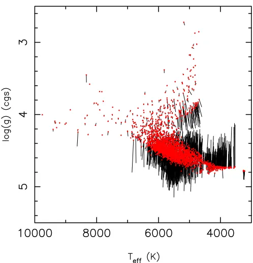
[image:9.612.319.568.51.310.2]whereδ represents the difference in the KIC and Yonsei–Yale parameter andσis the adopted uncertainty in the KIC parameter.
Figure 2.Surface gravity vs. effective temperature for the host stars. The red dots correspond to updated values based on a search of the Yonsei–Yale evolution models. Black lines point back to the locations defined by the KIC values. (A color version of this figure is available in the online journal.)
We adoptedσTeff =200 K,σlogg =0.3, andσ[Fe/H] =0.4 and
required the modeled age to be less than 14 Gyr. For each star we adopt the model-determined mass and radius. Figure2
showsTeffand logg. The red dots show updated values that have been adopted for determination of the stellar mass and radius. Stellar properties derived in this manner are flagged in Table3
by setting fTeff equal to 1. The black lines point to the star’s original location based on the KIC.
There are three populations that show significant changes to the determined logg. (1) Stars that fall below the main sequence move to smaller values of logg. These stars have Teff from roughly 4500 K to 6500 K. In general, estimates of the properties of these stars become larger and more luminous, which reduces the number of small stars and increases the amount of incident flux on the orbiting companion. (2) Most stars cooler than 4500 K see a substantial decrease in logg. However, modeled masses and radii are highly uncertain in this temperature range and should be used with caution. (3) There is a population of stars which have KIC loggnear 4.1 andTeffnear 5000 K. Stars in this region have no match when we restrict model ages to 14 Gyr. Such stars either move toward the red giant branch (lower values of logg) or toward the sub-giant branch (larger values of logg).
evolution model (Demarque et al. 2004) as described above for the KIC parameter adjustments. Stellar properties derived in this manner are flagged in Table3by settingfTeff equal to 3.
The spectra of 45 host stars were compared to a synthetic library of spectra as part of the Stellar Parameter Classification (SPC) effort and analysis tool described by Buchhave et al. (2012). As in the case of the SME analysis, the resulting stellar parameters are compared to the Yonsei–Yale models to determine the stellar radius. The revised stellar properties are listed in Table3and flagged withfTeffequal to 2.
Twenty-one host stars have neither KIC classifications nor spectroscopically derived stellar properties. In these cases (fTeff
equal to 0), the effective temperature is estimated from linear interpolation of the main-sequence properties of Schmidt-Kaler (1982) at the KICJ−Kcolor. There is little justification for the assumption of a main-sequence luminosity class. False positives and large errors in the planet candidate radius should be expected amongst this sample.
Also included in Table3 is the rms Combined Differential Photometric Precision (CDPP)—a measure of the photometric noise (including stellar and instrumental sources) on a 6 hr timescale after systematic-error correction and removal of strong sinusoidal features. A detailed description of the CDPP can be found in Jenkins et al. (2010b). CDPP values are crucial for statistical analyses of planet occurrence rates as they define the observational detection sensitivities. 3, 6, and 12 hr rms CDPP values for all observed stars are archived at MAST and can be obtained using the Data Retrieval Search form.
The objective of the Keplermission is to determine planet occurrence rate as a function of planet radius and orbital period. This requires accurate stellar properties not only of the planet-hosting stars but also of the parent population ofKepler target stars. The latter is required for sensitivity corrections. By including corrections to the properties of planet-hosting stars (or subsets thereof) and not the parent sample, we are introducing a non-uniformity that can negatively impact statistical studies.
Independent analyses of systematic errors in the KIC have begun to appear in the published literature. Muirhead et al. (2012a), for example, utilize medium-resolutionK-band spec-troscopy to asses systematic errors inTeff, logg, and [Fe/H] for late-K and M-type dwarfs amongst the sample of planet-hosting stars and report systematically overestimated stellar radii. Mann et al. (2012) perform a similar study of 382 target stars using medium-resolution optical spectra and show that the majority of bright (Kp < 14) and cool (Teff < 4500 K) stars in the Keplertarget catalog are giants. Pinsonneault et al. (2012) re-port on systematic errors in thegrizphotometry in the KIC used to determineTeff, logg, andRamong other parameters. These errors lead to underestimates in effective temperature.
The star properties listed in Table3do not contain corrections from these independent analyses. However, there is a concerted effort to devise a sensible strategy affecting future catalog releases—one that produces accurate estimates of star and planet properties while preserving uniformity for the purpose of statistical studies. A Kepler Star Properties Working Group has formed for this express purpose.32
In the meantime, we have checked for potential contamination of giants in the KOI sample using asteroseismology, which provides an effective means of identifying giant stars using Kepler data through the detection of solar-like oscillations
32 Information about allKeplerworking groups and how to participate can be found athttp://keplerscience.arc.nasa.gov.
(see, e.g., Gilliland et al.2010). Oscillation frequencies scale with effective temperature and surface gravity, and generally range from periods of a few minutes for main-sequence stars to several hours and longer for red giants (e.g., De Ridder et al.
2009; Chaplin et al. 2010). Red giants with logg 3.5 and Teff 5000 K oscillate at frequencies 300μHz, and hence oscillations for these stars are readily detectable with LCKepler data.
A preliminary analysis of all KOIs in the candidate cata-log using Q1–Q10 LC data yields only one detection of giant-like oscillations in a KOI classified as a main-sequence star: KOI-2548. However, there is a nearby foreground star approx-imately 4 mag brighter that has the same oscillation pattern as KOI-2548 and is classified as a giant in the KIC. High-resolution spectroscopy of KOI-2548 acquired with the HIRES spectrograph on the Keck telescope is consistent with a dwarf. The analysis confirms that the majority of KOI host stars are on or near the main sequence.
Note that there may be giants that have escaped detection due to close binary interactions suppressing the oscillations (Derekas et al.2011), but we suspect the number of such systems in the KOI catalog to be small. For stars withTeff 4000 K, the oscillation periods of potential giants would be too long to be sufficiently resolved with the amount of data currently available. Hence, the small number of KOIs in this temperature regime, particularly those with Kp < 14, should be viewed with caution. An in-depth asteroseismic study of KOIs using both short-cadence and long-cadence data will be presented in forthcoming papers.
5.3. Derived Parameters
The planet radius, semimajor axis, and equilibrium tempera-ture of each planet candidate are computed using the estimated stellar properties and the parameters returned by the light curve modeling described in Section5.1. Planet radius (Column 3 of Table5) is the product of the reduced radius,RP/R(Column 11 in Table4), and the stellar radius in Column 9 of Table3. Planet radii are given in units of Earth radii.
The semimajor axis provided in Column 4 of Table 5 is derived from Newton’s generalization of Kepler’s third law given the orbital period (Column 2) and the stellar mass (Column 10 of Table3). The stellar mass is derived directly from the surface gravity and stellar radius (Columns 8 and 9 of Table3). Although the parameterd/R(Column 9) is related to the reduced semimajor axis (a/R) as described in Section5.1, the two are only equivalent for the case of a circular orbit.
The equilibrium temperature, Teq (Column 5 of Table5) is the temperature at which the incident stellar flux balances the thermal radiation. It is derived by assuming that the planet and star act as gray bodies in equilibrium and that the heat is evenly distributed from the day to night side of the planet (e.g., a planet with an atmosphere or a planet with rotation period shorter than the orbital period):
Teq=Teff(R/2a)1/2[f(1−AB)]1/4, (3)
1
4
10
40
100
1
4
10
20
Period [days]
R p
/ R
e
Jupiter
Neptune
[image:11.612.124.494.55.323.2]Earth
Figure 3.Radius vs. orbital period for each of the planet candidates in the B10 (Borucki et al.2011a) catalog (blue points), the B11 (Borucki et al.2011b) catalog (red points), and this contribution (yellow points). Horizontal lines marking the radius of Jupiter, Neptune, and Earth are included for reference.
5.4. Period Aliasing
Section 4 describes the vetting procedures and the many metrics used to eliminate false positives. One of the statistics is a measure of the significance of odd/even depth differences. Aside from identifying eclipsing binaries, the metric can also be used as a warning that a low-S/N planetary period is a factor of two too low (as for KOI-730.03 and 191.04; Lissauer et al.
2011b). As an additional step outside the general procedures, we constructed a similar statistic for comparing the depths of every third or fourth transit. In this manner, the period of KOI-1445.02 was revised to be a factor of three larger than initial estimates (54 days compared to 18 days as determined the pipeline). Table 4 contains the updated period value. In this exercise we identified a handful of other planet candidates with low S/N, primarily based on one or two transits each,33 with ephemerides predicting transits that are not detected. When only two transits are seen, it is possible that each is associated with a distinct planet candidate that only transits once, or, alternatively, that they are the primary and secondary eclipse of an eccentric, long-period, blended eclipsing binary. In some cases, there may be an alternative orbital period that phases the observed transits with a gap in the data take. More observations are required to determine a unique solution. These period aliases show that while the catalog is generally of high reliability, additional analyses on the light curves of low-S/N transits may generate revisions.
6. DISTRIBUTIONS
The metrics and procedures described above, as applied to the Q1–Q6 data, yield 1108 new planet candidates, representing
33 KOI-2224.02, 1858.02, and 2410.02 have ephemerides indicative of two transits in the light curve; KOI-1070.03 and 2410.01 have ephemerides dominated by one transit apiece.
a gain of 88% over the B11 catalog. Eight of the new candidates are single-transit events (as indicated by negative, integer period values in Tables4and5). After removing the single-transit based candidates, the remaining candidates range in size from one-third the size of Earth to three times the size of Jupiter (transit depths of 20 parts per million to 20 parts per thousand) and equilibrium temperatures from 200 K to 3800 K (orbital periods of a half a day to nearly one year). Of the new candidates, 202, 422, 426, and 40 are Earth-size (RP <1.25R⊕), super-Earth-size (1.25R⊕ RP < 2R⊕), Neptune-size (2R⊕ RP < 6R⊕), and Jupiter-size (6R⊕ RP < 15R⊕), respectively. An additional 18 candidates are included in the catalog that are larger than 15R⊕, a small number of which are larger than three times the size of Jupiter and unlikely to be consistent with the planet interpretation. They are included here due to the uncertainties in the stellar radii (see Section5.2). Section7.3
describes the subsample of the new planet candidates that are in the HZ.
0 2 4 6 8 10 0
0.05 0.1 0.15 0.2 0.25
R
p/Re
N/N
tot
B11 New
0 20 40 60 80 100
0 0.05 0.1 0.15 0.2 0.25
Period [days]
B11 New
0 500 1000 1500 2000 2500 0
0.05 0.1 0.15
T
eq [K]
B11 New
30000 4000 5000 6000 7000 8000 0.05
0.1 0.15 0.2 0.25
T
eff [K]
N/N
tot
[image:12.612.52.559.58.373.2]B11 New
Figure 4.Radius, period, andTeqdistributions of the planet candidates in the B11 catalog (dark) and the new candidates presented here (light). The distribution of the surface temperature of their host stars is also included. Counts are expressed as fractions of the total number of candidates in each of the two catalogs.
(A color version of this figure is available in the online journal.)
The relative gains in the number of candidates are displayed in Figure4, which contains normalized distributions of planet ra-dius, period, equilibrium temperature, and host star temperature for the B11 catalog and for the new candidates presented here. In terms of radius, the gains are predominantly for candidates smaller than 2R⊕. The new candidates contain a significantly smaller fraction of Neptune-size and Jupiter-size planets than the 2011 February catalog. We report a growth of 201% for candidates smaller than 2R⊕ compared to 53% for candidates larger than 2R⊕, and a growth of 124% for orbital period longer than 50 days compared to an 86% increase for periods shorter than 50 days. The gains in equilibrium temperature and host star properties are more uniform (approximately 88% for most bins). Section7.1compares these gains to what would be ex-pected from increasing the baseline observation window from 13 months (Q1–Q5) to 16 months (Q1–Q6).
7. DISCUSSION
7.1. Computed versus Observed Growth in Numbers of Candidates
We compare the observed gain in the numbers of candidates to that expected from an increase in sensitivity afforded by three additional months of data. To do so, we develop a simplified model for the expected detection of transiting planets with Keplerdata following Burke et al. (2006) whereby the detection probability is separated into two independent terms: probability for detection from a sensitivity (S/N) standpoint and probability for geometric alignment to transit.
The first term determines whether the data have sufficient photometric precision and number of observed transit events for detection above theσthresh=7.1 significance threshold adopted by the mission (Jenkins2002). We estimate the total S/N of a transit sequence of depth,Δ, and orbital period,Porbas
S/N= Δ σcdpp
Nevents, (4)
where σcdpp is the observed photometric noise for a given star on a timescale comparable to the transit duration. The duration is computed for a given stellar mass and assuming a circular orbit with period, Porb, and an impact parameter b = (π/4) corresponding to the expectation value for an isotropic distribution of angular momentum vectors. The TPS pipeline algorithm measuresσcdppover a grid of transit durations from 1.5 to 15.0 hr (Jenkins 2002; Christiansen et al. 2012), and we interpolate to determine the photometric noise at the estimated duration expected. The expected number of transit events is given by
Nevents=ηTobs Porb
, (5)
whereη=0.95 is the duty cycle of the photometric time series andTobsis the duration of the observations.
Orbital Period [day]
Planet Radius [R
]
10 20 40 65 100 150 200
0.85 1 1.25 1.6 2 2.6
[image:13.612.320.566.55.242.2]10 20 30 40 50 60 70 80 90
Figure 5.Detection probability (expressed as percent completeness) contours as a function of planet radius and orbital period for a Kp=12 mag star with the properties listed in Table6.
cumulative Gaussian distribution aboveσthresh=7.1:
PS/N= 1 2+
1 2erf
(S/N−σthresh)
√
2.0
. (6)
We construct a grid of such probabilities as a function of transit depth and orbital period. Figure 5 shows a sample grid for a typical Kp= 12 magnitude star assuming five quarters of observations (407 days) and a 95% duty cycle. The grid is displayed as contours of equal detection probability, or “percent completeness.”
The TPS algorithm as implemented requires a minimum of three transit events for detection. To account for this in the detection probability we model the decrease in sensitivity toward longerPorbby determining thePorb,3 whenNevents =3 and Porb,2 when Nevents = 2. The detection probability then linearly decreases from 1.0 to 0.0 probability over the range Porb,3 PorbPorb,2. This modeling of requiring three transits in the detection probability results in the apparent “upturn” of the detection probability contours at the longest orbital periods in Figure5.
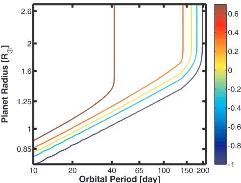
The product of the detection probability and the probability of geometric alignment yields the total detection probability. The geometric alignment probability is proportional to the ratio of the stellar radius and planet–star separation normalized to 0.46% for an Earth–Sun analog. Figure6displays (logarithmic) completeness contours for the same Kp=12 star after including the geometric alignment probability. From left to right, the contours are 5.0%, 2.0%, 1.0%, 0.5%, and 0.1%, or 0.7, 0.3, 0.0,
−0.3, and−1, respectively, on the logarithmic scale. If nature produces planets that uniformly populate the radius/period plane with circular orbits, then the planets detected byKepler will be distributed similarly to the contours shown.
Instead of computing a grid of total detection probabilities for each of the>150,000 stars in the parent sample, we devise a representative sample. Stars observed byKepler, in the range 4.0<logg <4.9 andR<1.4, are sorted into Kp=0.25 mag bins, excluding those that do not have stellar classifications in the KIC. This results in 145,728 targets with 10.75<Kp<17.75. Table6lists the number of stars in each magnitude bin together with the median stellar radius for that bin. The associated loggandTeff are interpolated of Tables 15.7 and 15.8 in Cox
Orbital Period [day]
Planet Radius [R
]
10 20 40 65 100 150 200
0.85 1 1.25 1.6 2 2.6
-1 -0.8 -0.6 -0.4 -0.2 0 0.2 0.4 0.6
[image:13.612.47.294.58.246.2]Figure 6.Probability contours displayed in Figure5are corrected for the geo-metric alignment probability (normalized to the geogeo-metric alignment probability of an Earth/Sun analog: 0.00465). These alignment-corrected probability con-tours are displayed here. The colors of the concon-tours are mapped to the logarithm of the probability. These values, from left to right are 0.7, 0.3, 0.0,−0.3, and−1.
Table 6
The Parent Star Sample: Representative Properties and Star Counts
Kp R logg Teff Nstars CDPPa
11 1.144 4.3689 6055.0 315 23.3
11.5 1.394 4.3440 6968.3 1282 27.4
12 1.32 4.3462 6737.4 2327 31.1
12.5 1.273 4.3481 6545.2 4177 36.9
13 1.204 4.3547 6268.2 7272 44.5
13.5 1.139 4.3705 6039.7 11892 55.2
14 1.028 4.4303 5833.3 14961 69.0
14.5 0.947 4.4744 5667.0 19340 92.0
15 0.922 4.4816 5569.2 29831 123.3
15.5 0.867 4.4856 5257.2 36818 168.9
16 0.781 4.5081 4741.3 15900 221.2
16.5 0.745 4.5249 4543.1 873 378.5
17 0.738 4.5283 4505.5 603 532.6
17.5 0.775 4.5107 4707.6 137 876.6
Note.a30thpercentile of the 6 hr CDPP values (in parts per million) of all stars in the relevant magnitude bin.
(2000). The photometric noise taken as the 30th percentile of the 6 hr CDPP values34 of the targets in the magnitude bin. The stellar properties associated with the Kp = 12 mag bin are those used for the calculations that produced the results displayed in Figures5 and6. Though the majority of Kepler targets are G-type stars on or near the main sequence (Batalha et al. 2010b), it is evident from Table6 that the median star type depends on magnitude. We assume that all stars in the magnitude bin can be represented by the properties tabulated. Though insufficient for computingKepler’s detection efficiency in an absolute sense, this assumption is a useful simplification for exploring the expected planet yield in a relative sense.
The total planet yield for a given magnitude bin is computed by taking the product of the alignment-corrected detection probability and the number of targets in that magnitude bin.
[image:13.612.318.568.332.495.2]