Robust Neurofuzzy Rule Base Knowledge Extraction
and Estimation Using Subspace Decomposition
Combined With Regularization and D-Optimality
Xia Hong
, Senior Member, IEEE
, Chris J. Harris, and Sheng Chen
, Senior Member, IEEE
Abstract—A new robust neurofuzzy model construction algo-rithm has been introduced for the modeling ofa prioriunknown dynamical systems from observed finite data sets in the form of a set of fuzzy rules. Based on a Takagi–Sugeno (T–S) inference mechanism a one to one mapping between a fuzzy rule base and a model matrix feature subspace is established. This link enables rule based knowledge to be extracted from matrix subspace to enhance model transparency. In order to achieve maximized model robust-ness and sparsity, a new robust extended Gram–Schmidt (G–S) method has been introduced via two effective and complementary approaches of regularization and D-optimality experimental de-sign. Model rule bases are decomposed into orthogonal subspaces, so as to enhance model transparency with the capability of inter-preting the derived rule base energy level. A locally regularized orthogonal least squares algorithm, combined with a D-optimality used for subspace based rule selection, has been extended for fuzzy rule regularization and subspace based information extraction. By using a weighting for the D-optimality cost function, the entire model construction procedure becomes automatic. Numerical ex-amples are included to demonstrate the effectiveness of the pro-posed new algorithm.
Index Terms—Neurofuzzy networks, optimal experimental de-sign, orthogonal decomposition, regularization, subspace.
I. INTRODUCTION
A
SSOCIATIVE memory networks [such as B-spline net-works, radial basis functions (RBFs), support vector ma-chines (SVM)] have been extensively developed [1]–[4]. Most conventional neural networks lead only to “black box” model representation, yet a neurofuzzy network has an inherent model transparency that helps users to understand the system behav-iors, oversee critical system operating regions, and/or extract physical laws or relationships that underpin the system. Based on the fuzzy rules inference and model representation of Takagi and Sugeno (T–S) [5], a neurofuzzy model can be functionally expressed as an operating point dependent fuzzy model with a local linear description that lends itself directly to conventional estimation and control synthesis [1], [6], [7]. The model output is decomposed into a convex combination of the outputs of in-dividual rules, and the basis function can be interpreted as aManuscript received December 11, 2002; revised June 4, 2003. This work was supported in part by the EPSRC, U.K. This paper was recommended by Associate Editor D. Nauck.
X. Hong is with Cybernetic Intelligence Research Group, Department of Cybernetics University of Reading, Reading, RG6 6AY, U.K. (e-mail: [email protected]).
C. J. Harris and S. Chen are with the Department of Electronics and Computer Science University of Southampton, Southampton SO17 1BJ, U.K.
Digital Object Identifier 10.1109/TSMCB.2003.817089
fuzzy membership function of individual rules. This property is critically desirable for problems requiring insight into the un-derlying phenomenology, i.e., internal system behavior inter-pretability and/or knowledge (rule) representation of the under-lying process.
The problem of the curse of dimensionality[8] has been a main obstacle in nonlinear modeling using associative memory networks or fuzzy logic. Networks or knowledge representa-tions that suffer from the curse of dimensionality include all lattice based networks such as fuzzy logic (FL), RBF, Karneva distributed memory maps, and all neurofuzzy networks (e.g. adaptive network based fuzzy inference system (ANFIS) [9], T–S model [5], etc.). This problem also mitigates against model transparency for high dimensional systems since they generate massive rule sets, or require too many parameters, making it im-possible for a human to comprehend the resultant rule set. Con-sequently the major purpose of neurofuzzy model construction algorithms is to select a parsimonious model structure that re-solves the bias/variance dilemma (for finite training data), has a smooth prediction surface (e.g. parameter control via regulariza-tion), produces good generalization (for unseen data), and with an interpretable representation—often in the form of (fuzzy) rules. For general linear in the parameter systems, an orthogonal least squares (OLS) algorithm based on Gram-Schmidt (G–S) orthogonal decomposition can be used to determine the models significant elements and associated parameter estimates, and the overall model structure [10]. Regularization techniques have been incorporated into the OLS algorithm to produce a regular-ized orthogonal least squares (ROLS) algorithm that reduces the variance of parameter estimates [11], [12]. To produce a model with good generalization capabilities, model selection criteria such as the Akaike information criterion (AIC) [13] are usually incorporated into the procedure to determinate the model con-struction process. Yet the use of AIC or other information based criteria, if used in forward regression, only affects the stopping point of the model selection, but does not penalize regressors that might cause poor model performance, e.g., too large param-eter variance or ill-posedness of the regression matrix, if this is selected. This is due to the fact that AIC or other information based criteria are usually simplified measures derived as an ap-proximation formula that is particularly sensitive to model com-plexity.
In order to achieve a model structure with improved model generalization, it is natural that a model generalization ca-pability cost function should be used in the overall model searching process, rather than only being applied as a measure
of model complexity. Optimum experimental designs have been used [14] to construct smooth network response surfaces based on the setting of the experimental variables under well controlled experimental conditions. In optimum design, model adequacy is evaluated by design criteria that are statistical mea-sures of goodness of experimental designs by virtue of design efficiency and experimental effort. Quantitatively, model ade-quacy is measured as function of the eigenvalues of the design matrix. In recent studies [15], [16], the authors have outlined efficient learning algorithms, in which composite cost functions were introduced to optimize the model approximation ability using the forward orthogonal least squares (OLS) algorithm [10], and simultaneously determined model adequacy using an A-optimality design criterion (i.e., minimizes the variance of the parameter estimates), or a D-optimality criterion (i.e., optimizes the parameter efficiency and model robustness via the maximization of the determinant of the design matrix). It was shown that the resultant models can be improved based on A- or D-optimality. These algorithms lead automatically to an unbiased model parameter estimate with an overall robust and parsimonious model structure. Combining a locally regularized orthogonal least squares (LROLS) model selection [17] with D-optimality experimental design further enhances model robustness [18].
Due to the inherent transparency properties of a neurofuzzy network, a parsimonious model construction approach should lead also to a logical rule extraction process that increases model transparency, as simpler models inherently involve fewer rules which are in turn easier to interpret. One drawback of most current neurofuzzy learning algorithms is that learning is based upon a set of one-dimensional (1-D) regressors, or basis functions (such as B-splines, Gaussians, etc), but not upon a set of fuzzy rules (usually in the form of multidimensional input variables), resulting in opaque models during the learning process. Since modeling is inevitably iterative it can be greatly enhanced if the modeller can interpret or interrogate the derived rule base during learning itself, allowing him/her to terminate the process when his/her objectives are achieved. There are valuable recent developments on rule based learning and model construction, including a linear approximation approach combined with uncertainty modeling [19], various fuzzy sim-ilarity measures combined with genetic algorithms [20], [21]. Recently the authors have introduced a new neurofuzzy model construction and parameter estimation algorithm from observed finite data sets, based on a T–S inference mechanism and a new extended G–S orthogonal decomposition algorithm, for the modeling ofa prioriunknown dynamical systems in the form of a set of fuzzy rules [22], which, based on a T–S inference mechanism, establishes a one to one mapping between a fuzzy rule base and a model matrix feature subspace.
In this paper, a new neurofuzzy model construction and pa-rameter estimation algorithm has been introduced. Based on a T–S inference mechanism a one to one mapping between a fuzzy rule base and a model matrix feature subspace is estab-lished [22]. This link enables rule based knowledge to be ex-tracted from matrix subspace to enhance model transparency. In order to achieve maximized model robustness and sparsity, a new robust extended G–S algorithm has been introduced via two
effective and complementary approaches of regularization and D-optimality experimental design. This new algorithm poses the model rule bases via an orthogonal subspace decom-position approach, so as to enhance model transparency with the capability of interpreting the derived rule base energy level. A locally regularized orthogonal least squares algorithm tailored for rule regularization has been combined with a D-optimality for subspace selection. By using a weighting for the D-opti-mality cost function, the entire model construction procedure becomes automatic. The proposed algorithm enhances the pre-vious algorithm [22] via the combined LOLS and D-optimality for robust rule selection, and is based on the extension of the combined LOLS and D-optimality algorithm [18] from conven-tional regressor regression to orthogonal subspace regression.
This paper is organized as follows. Section II introduces a general class of neurofuzzy systems as a modeling approach. Section III introduces the proposed new algorithm, with analysis into the associated model transparency, robustness enhancement via D-optimality and rule based regularization. Numerical ex-amples are provided in Section IV to illustrate the effectiveness of the approach and Section V is devoted to conclusions.
II. A NEUROFUZZYMODELINGAPPROACH
This section briefly presents a general class of neurofuzzy systems as a nonlinear data modeling approach within a coherent framework of both mathematical representation for learning and linguistic logic rule representation for model
transparency. Given a finite data set of
observed input/output data pairs, consider the identification of a general nonlinear system that generates this data
(1)
where
(2)
is an observed system input vector, isa prioriunknown. The observation noise is assumed uncorrelated with vari-ance . is an unknown parameter vector associated with an appropriate but yet to be determined model structure.
Model (1) can be simplified by decomposing it into a set of
local models , , where is to be
determined, each of which operates on a local region depending on the submeasurement vector , a subset of the input
vector , i.e., , , .
Each of the local models can be represented by a set of linguistic rules
(3)
where the fuzzy set denotes a fuzzy
set in the -dimensional input space, and is given as an array of linguistic values, based on a predetermined input spaces partition into fuzzy sets via some prior system knowledge of the operating range of the data set. Usually if , for
defines a complete fuzzy partition of the input space . For an appropriate input space decomposition, the local models can have essentially local linear behavior. In this case, using the well known T–S fuzzy inference mechanism [5], the output of system (1) can be represented by
(4)
where is a linear function of , given by
(5)
and denotes parameter vector of the th fuzzy rule or local model. is a fuzzy membership function of the rule (3), subject to a unity of support condition: , . Each of the linguistic rules (3) can be eval-uated via the known fuzzy membership function .
Consider a neurofuzzy network using B-spline functions [23] as membership functions. A general 1-D B-spline model can be formed as a linear combination of B-spline basis
func-tions, , as
(6)
The coefficients ’s represent the set of adjustable parameters associated with the set of basis functions. ’s, which are polynomials of a given degree and are uniquely defined by an ordered sequence of real values denoted as a knot vector
. The knot sequence forms a partitioning of the input domain into disjoint intervals. The basis functions set can be defined by recursive equation [23]
(7) with
otherwise.
Multidimensional B-spline basis functions are formed by a di-rect multiplication of univariate basis functions via
(8)
for , where ,
. , is the
number of B-spline basis functions defined in , the th component of .
Note that for a complete model base, the number of rules increases exponentially as the input dimension in-creases, (which is commonly known as the curse of dimension-ality). To alleviate this disadvantage, input dimension or vari-able reduction can be used. Notably an ANOVA (analysis of variance) representation of multivariable functions uses lower dimensional tensor products of models inputs, e.g. in many prac-tical applications, the number of multiplication terms maybe
limited to as low as 3, yet maintaining sufficient modeling ca-pability [1]. For practical applications, not only is the ANOVA approach effective in overcoming the curse of dimensionality, it has additional advantage of model transparency because a lower input dimension than three can be visualized and interpreted [24].
Substitute (5) and (4) into (1):
(9)
where
. .
, where .
For the finite data set , (9) can be
written in a matrix form as
(10)
where is the output
vector, is
the regression matrix associated with the th fuzzy rule, is the model residual vector. is the full regression matrix. An effective way of overcoming the curse of dimensionality is to start with a moderate sized rule base according to the actual data distribution. In this paper, the selection of local models as an initial model base is based on model identifiability via an A-optimality design criterion [14] with the advantage of en-hanced model transparency to quantify and interpret fuzzy rules and their identifiability.
III. RULEBASED MODEL CONSTRUCTION AND
LEARNINGALGORITHMS
A. Rule Based Learning and Initial Model Base Construction
Rule based knowledge, i.e., information associated with a fuzzy rule, is highly appropriate for users to understand a de-rived data based model. Most current learning algorithms in neurofuzzy model are based on an ordinary p-dimensional linear in the parameter model. Model transparency during learning cannot be automatically achieved unless these regressors have a clear physical interpretation, or are directly associated with physical variables. Alternatively, a neurofuzzy network is in-herently transparent for rule based model construction. In (10), each of is constructed based on a unique fuzzy membership function , providing a link between a fuzzy rule base and a matrix feature subspace spanned by . Rule based knowl-edge can be easily extracted by exploring this link.
Definition 1: Basis of a Subspace: If vectors , , satisfy the nonsingular condition that
has a full rank of , they span a -di-mensional subspace , then is the basis of the subspace
Definition 2: Fuzzy Rule Subspace: Suppose the is non-singular, clearly is the basis of a -dimensional subspace , which is a functional representation of the fuzzy rule (3) by using T–S fuzzy inference mechanism with a unique label . is defined as a fuzzy rule subspace of the th fuzzy rule.
, the submatrix associated with the th rule, can be ex-panded as
(11)
where ,
. (11) shows that each rule base is simply constructed by a weighting matrix multiplied to the regression matrix of original input variables. The weighting matrix can be regarded as a data based spatial prefiltering over the input region. Without loss of generality, it is assumed that is nonsingular, and ,
as . As
(12)
For to be nonsingular, then , this means
that for the input region denoted by , its basis function needs to be excited by at least data points.
The A-optimality design criteria for the weighting matrix which is given by [14], [22]
(13)
provides an indication for each fuzzy rule on its identifiability and hence a metric for selecting appropriate model rules. The derived model rules can then be rearranged in descending order of identifiability, followed by utilizing only the first experts with identifiability to construct a model rule base set.
B. Orthogonal Subspace Decomposition and Regularization in Orthogonal Subspace
For ease of exposition, we initially introduce some notations and definitions that are used in the development of the new ex-tended G–S orthogonal decomposition algorithm.
Definition 3: Orthogonal Subspaces: For a -dimensional matrix space , two of its subspaces
and , ( , ) are orthogonal if
and only if any two vectors and that are located in the
two subspaces respectively, i.e., and ,
are orthogonal, that is, , for .
The -dimensional space , , can be
decom-posed by orthogonal subspaces , , given
by [25], [26]
(14)
where denotes sum of orthogonal sets. From Definition 1, if there are any linear uncorrelated vectors located in ,
de-noted as , , then the matrix
, forms a basis of . Note that these vec-tors need not to be mutually orthogonal, i.e.,
, where is not required to be diagonal. Clearly if two matrix subspaces , have the basis of
full rank matrices , , then they
are orthogonal if and only if
(15)
where is a zero matrix.
Definition 4: Vector Decomposition to Subspace Basis: If orthogonal subspaces , , are defined by a
series of matrices , as subspace basis
based on Definition 3, then an arbitrary vector can be uniquely decomposed as
(16)
where ’s are combination coefficients.
.
As the result of the orthogonality of , (for ), from (16),
(17)
Clearly the variance of the vector projected into each subspace
can be computed as , for .
Consider the nonlinear system (1) given as a vector form by (10). By introducing an orthogonal subspace decomposition
, (10) can be written as
(18)
where spans a -dimensional space
with , spanning its subspaces , as
defined via Definition 3. The auxiliary parameter vector , where is a block upper trian-gular matrix
(19)
in which . , a unit matrix
.
model (18) can be realized based on an extended G–S orthog-onal decomposition algorithm as follows. Set ,
, and, for , set ,
(20)
where
(21)
for .
Definition 6: Locally Regularized Least Squares Cost Func-tion in Orthogonal Subspaces: The orthogonal subspace based regularized least squares uses the following error criterion:
(22)
where , ,
are regularization parameters, and the diagonal matrix , is a unit matrix. The regularized least squares estimates of , is given by [27]
(23)
An appropriate choice of can smooth parameter estimates (noise rejection), and can be optimized by using a separate procedure, such as Bayesian hyper-parameter optimization [18], or a genetic algorithm. In this paper, it is assumed that an appro-priate is predetermined to simplify the procedure. The regu-larized least squares solution of (18) is given by
(24)
which follows from the fact that , are
mu-tually orthogonal subspaces basis, and .
From (16), if the system output vector is decomposed as a term by projecting onto orthogonal subspaces , , and an uncorrelated term that is unexplained by the model, such that the projection onto each subspace basis (or a per-centage energy contribution of these subspaces toward the con-struction of ) can be readily calculated via
(25)
[image:5.612.312.537.65.196.2]The output variance projected onto each subspace can be in-terpreted as the contribution of each fuzzy rule in the fuzzy system, subject to the existence of previous fuzzy rules. To in-clude the most significant subspace basis with the largest as a forward regression procedure is a direct extension of con-ventional forward OLS algorithm [10]. The output variance pro-jected into each subspace can be interpreted as the output energy contribution explained by a new rule demonstrating the signifi-cance of the new rule toward the model. At each regression step, a new orthogonal subspace basis is formed by using a new fuzzy
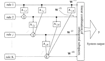
Fig. 1. Orthogonal subspace decomposition based on fuzzy rule bases.
rule and the existing fuzzy rules in the model, with the rule basis with the largest to be included in the final model until
(26)
satisfies for an error tolerance to construct a model with rules. The parameter vectors , can be com-puted by the following back substitution procedure: Set
, and, for
(27)
The concept of orthogonal subspace decomposition based on fuzzy rule bases is illustrated in Fig. 1. This figure illustrates (20) that forms the orthogonal bases. Because of the one to one mapping of a fuzzy rule to a matrix subspace, a series of orthog-onal subspace basis are formed by using fuzzy rule subspace basis in a forward regression manner, such that,
, , whilst maxi-mizing the output variance of the model at each regression step . Note that the well known orthogonal schemes such as the clas-sical G–S method construct orthogonal vectors as basis based on regression vectors (1-D), but the new algorithm extends the classical G–S orthogonal decomposition scheme to the orthogo-nalization of subspace bases (multidimensional). The extended G–S orthogonal decomposition algorithm is not only an exten-sion from classical G–S orthogonal axis decomposition to or-thogonal subspace decomposition, but also as an extension from basis function regression to matrix subspace regression, intro-ducing a significant advantage of model transparency to inter-pret fuzzy rule energy level.
C. New Extended G–S Orthogonal Decomposition Algorithm With Regularization and D-Optimality in Orthogonal Subspaces
as least squares plus a penalty term based D-optimality experi-mental design criterion can be used [16]. To enhance rule model robustness, the proposed algorithm combines the two separate previous works, the subspace based rule based model construc-tion [22] and the combined LOLS and D-optimality algorithm [18] for robust rule based model construction. The combined LOLS and D-optimality algorithm [18] was not previously in-troduced as a rule based learning algorithm, hence some exten-sions to orthogonal subspace decomposition domain are neces-sary, as introduced in the following.
The concept of parameter regularization may be incorporated into a forward orthogonal least squares algorithm as a locally regularized orthogonal least square estimator for subspace se-lection by defining a regularized error reduction ratio due to the submatrix as follows.
After some simplification, it can be shown that the criterion (22) can be expressed as
(28)
where . Normalizing (28) by yields
(29)
The regularized error reduction ratio due to the subma-trix
(30)
Definition 7: D-Optimality Experimental Design Cost Func-tion in Orthogonal Subspaces: In experimental design, the data covariance matrix is called the design matrix. The D-op-timality design criterion maximizes the determinant of the de-sign matrix for the constructed model. Consider a model with orthogonal subspaces with design matrix as , and a subset of these subspaces are selected in order to construct a -subspace model that maximizes the D-optimality , where is a column subset of repre-senting a constructed subset model with submatrices selected from (consisting of submatrices). It is straightforward to verify that the maximization of is
equiva-lent to the minimization of [22].
Clearly
(31)
It can be easily verify that the maximization of is identical to the maximization of
, where is a column subset of ( rep-resenting a constructed subset model with submatrices selected from (consisting of submatrices) [22].
Definition 8: Combined Locally Regularized Cost Function and D-Optimality in Orthogonal Subspaces: The combined LROLS and D-optimality algorithm based on orthogonal subspace decomposition is based on the combined criterion
(32)
for model selection, where is a fixed small positive weighting for the D-optimality cost. Equivalently a combined error reduc-tion ratio defined as
(33)
is used for model selection, and the selection is terminated with a -subspace model when
(34)
The introduction of D-optimality enhances model robustness and simplify the model selection procedure [18]. Given a proper , the new extended G–S orthogonal subspace decomposition algorithm with regularization and D-optimality for rule based model construction is given in Appendix I.
IV. NUMERICALEXAMPLES
Example 1: We start with a simple illustrative mapping ex-ample. Consider a nonlinear functional approximation of
Five–hundred data pairs are generated where the system input is generated as a uniformly distributed random number ranged in [0,1]. Define a knot vector [ 0.2,0,0.2,0.4,0.6,0.8,1,1.2], and use a piecewise linear B-spline fuzzy membership function to build a 1-D model, resulting basis functions. These basis functions, as shown in Fig. 2, corresponding to six fuzzy rules. 1) If
(very small); 2) IF (small); 3) IF
(medium-small); 4) IF (medium-large); 5) IF (large); and 6) If (very large).
By using the fuzzy model (4) for the approximation of , the neurofuzzy model is simply given as
(35)
Fig. 2. Fuzzy membership functions forxin Example 1. TABLE I
FUZZYRULESIDENTIFIABILITY INEXAMPLE1
TABLE II
SYSTEMERRORREDUCTIONRATIO BY THESELECTEDRULES INEXAMPLE1
TABLE III
MODELMEANSQUARESERRORS(MSE)FORNOISYOBSERVATIONS ANDUNDERLYINGFUNCTION
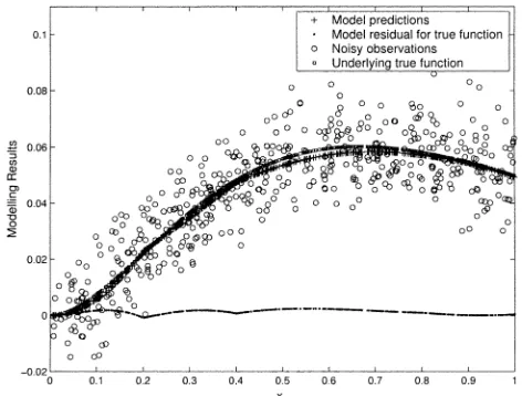
(in the order of selected rules), shown in two cases of with or without parameter regularization. Each rule contribution in reducing model error (or increasing the model energy level) provides model transparency for the fuzzy rules interpretability. To verify the model’s approximation and robustness, Table III lists the mean squares error (MSE) of model in target to the noisy observations and the true function , respec-tively. For this example, the modeling results are insensitive to a wide range of the parameter associated with D-optimality
( ). However for , the model
selection process automatically terminates at a five-rule model (rule 1 is excluded). This insensitivity means that varying within a certain range will all terminates the modeling within a suitable structural range. The modeling results of a
Fig. 3. Modeling results of a five-rule model with = 0:2for Example 1.
model using five rules with is plotted in Fig. 3. This example demonstrates that the proposed method has good approximation and some robustness improvement. Clearly the proposed modeling approach is additionally advantageous via its significant model transparency during the modeling process.
Example 2: Nonlinear 2-D Surface Modeling: The Matlab logo was generated by the first eigenfunction of the L-shaped membrane. A 51 51 meshed data set is generated by using Matlab commands
(36)
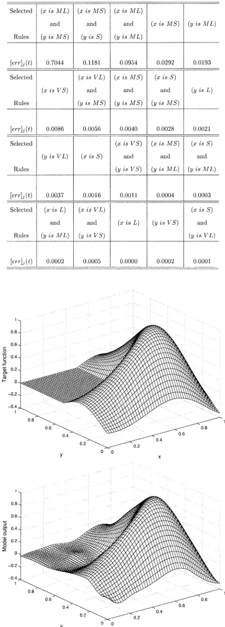
such that output is defined over an unit square input region . The data set , shown in Fig. 5(a), is used to model the target function (the first eigenfunction of the L-shaped mem-brane function).
For both , , define a knot vector [ 0.4, 0.2,0,0.25,0.5,0.75,1,1.2,1.4], and use a piecewise quadratic B-spline fuzzy membership function to build a 1-D model, resulting basis functions. These basis functions, as shown in Fig. 4, correspond to six fuzzy rules. 1) If ( or ) is (very small) (VS); 2) IF ( or ) is (small)(S); 3) IF ( or ) is (medium-small)(MS); 4) IF ( or ) is (medium-large)(ML); 5) IF ( or ) is (large)(L); and 6) If ( or ) is (very large)(VL).
The univariate and bivariate membership functions (interac-tion between univariate membership func(interac-tion and via tensor product) are used as model set and shown in Table IV, in which, the identifiability of fuzzy rules are listed based on (13). From Table IV, it is seen that all the rules have been uniformly excited. There are 48 rules.
By using the fuzzy model (4) for the modeling of , the neurofuzzy model is simply given as
(37)
[image:7.612.49.286.61.247.2]Fig. 4. Fuzzy membership functions forx, oryin Example 2. TABLE IV
FUZZYRULESIDENTIFIABILITY INEXAMPLE2; (A) RULESABOUTx; (B) RULESABOUTy; (C) RULESABOUT X AND Y(THESTAR“ ” INDICATES
RULESINCLUDED IN THEFINALMODEL)
of the fuzzy rule spans a two-dimensional (2-D) space, i.e., , . The proposed algorithm based on the extended G–S orthogonal decomposition has been applied, in which each rule subspace being spanned by a 2-D rule basis is mapped into orthogonal matrix subspaces. The modeling re-sults contain rule based information of percentage energy incre-ment (or the model error reduction ratio) by the selected rule
to the model as shown in Table V for , .
[image:8.612.310.542.89.733.2]The MSE of the resultant 20-rule model is . In Table V, the selected rules are ordered in the sequence of being selected, and the model selection automatically terminates at a 20-rule model . The model prediction of the 20-rule model is shown in Fig. 5(b). For this example, the mod-eling results are insensitive to value of . It has shown that by
TABLE V
SYSTEMERRORREDUCTIONRATIO BY THESELECTEDRULES INEXAMPLE2
TABLE VI
SYSTEMERRORREDUCTIONRATIO BY THESELECTEDRULES INEXAMPLE3
Fig. 6. Modeling results for Example 3.
using a weighting for the D-optimality cost function, the entire model construction procedure becomes automatic. It can be seen that the model has some limitations over the modeling of corner and edge of the surface due to the data being only piecewise smooth and piecewise nonlinear. This factor may contribute to the fact that regularization may not help in reducing misfit in some strong nonlinear behavior region. Global nonlinear mod-eling using B-spline for strong nonlinear behavior such as piece-wise smooth and piecepiece-wise nonlinear data is under investiga-tion.
Example 3: Consider the benchmark Henon time series given by
(38)
Five-hundred data points are generated with an initial
con-dition , . All the data points were used
in the modeling by using the proposed approach. The mod-eling process is briefly described here. The input vector . For each input, define a knot vector [ 2.0, 1.9, 1.8,0,1.8,1.9,2.0], and use a piecewise quadratic B-spline fuzzy membership function to build a 1-D
model, resulting basis functions, corresponding to six fuzzy rules. That is, for : 1) If is (small) (S); 2) If is (Medium Small) (MS); 3) If
is (Medium Large) (ML); 4) If is (Large) (L); Then bivariate membership functions are formed by using tensor product.
The modeling results derived by the subspace forward
re-gression process, with , , is given in
Table VI, with the final model consisting of 13 fuzzy rules. This table shows the energy level per rule extracted for this chaotic time series. Fig. 6 demonstrates the excellent approximation of the derived model. The final model MSE is 0.0041. This is very small compared to signal variance of 1.01.
V. CONCLUSIONS
This paper has introduced a new robust neurofuzzy model construction algorithm for the modeling ofa prioriunknown dynamical systems in the form of a set of fuzzy rules. A one to one mapping between a fuzzy rule base and a model matrix feature subspace has been established by extending a T–S in-ference mechanism. Rule based knowledge are extracted from matrix subspace to enhance model transparency due to this map-ping link. In order to achieve maximized model robustness and sparsity, a new robust extended G–S method has been intro-duced via two effective and complementary approaches of regu-larization and D-optimality experimental design. By combining a subspace approach and the concept of robust model construc-tion, a locally regularized orthogonal least squares algorithm is extended for fuzzy rule regularization and subspace based in-formation extraction, and by combined with a D-optimality for subspace based rule selection. Model rule bases are decomposed into orthogonal subspaces, so as to enhance model transparency with the capability of interpreting the derived rule base energy level, and are automatically selected for a model with robust-ness.
APPENDIX I
THEALGORITHM
An extended classical G–S scheme combined with parameter regularization and D-optimality selective criterion in orthogonal subspaces can be summarized as the following procedure.
1) At the th forward regression step, where , for , compute
for and if if
if if
(39)
(41)
Find
for rule base selection (42)
and select
for selected rule base energy
level information extraction (43)
The selected submatrix exchanges columns with submatrix . For notational convenience, all the sub-matrices will still be referred as , , ac-cording to the new column submatrix order in , even if some of the column submatrices have been interchanged. 2) The procedure is monitored and terminated at the derived step, when , for a predetermined . Otherwise, set , go to step 1.
3) Calculate the original parameters according to (27).
ACKNOWLEDGMENT
X. Hong gratefully acknowledges the EPSRC, U.K. The au-thors would like to thank the referees for the constructive com-ments.
REFERENCES
[1] C. J. Harris, X. Hong, and Q. Gan,Adaptive Modeling, Estimation and Fusion From Data: A Neurofuzzy Approach. Berlin, Germany: Springer-Verlag, 2002.
[2] M. Brown and C. J. Harris,Neurofuzzy Adaptive Modeling and Con-trol. Hemel Hempstead, U.K.: Prentice-Hall, 1994.
[3] K. M. Bossley, “Neurofuzzy Modeling Approaches in System Identifi-cation,” Ph.D. thesis, Dept. ECS, Univ. Southampton, U.K., 1997. [4] R. Murray-Smith and T. A. Johansen,Multiple Model Approaches to
Modeling and Control. London, U.K.: Taylor and Francis, 1997. [5] T. Takagi and M. Sugeno, “Fuzzy identification of systems and its
ap-plications to modeling and control,”IEEE Trans. Syst., Man, Cybern., vol. SMC-15, pp. 116–132, 1985.
[6] M. Feng and C. J. Harris, “Adaptive neurofuzzy control for a class of state-dependent nonlinear processes,”Int. J. Syst. Sci., vol. 29, no. 7, pp. 759–771, 1998.
[7] H. Wang, M. Brown, and C. J. Harris, “Modeling and control of non-linear, operating point dependent systems via associative memory net-works,”J. Dynam. Contr., vol. 6, pp. 199–218, 1996.
[8] R. Bellman, Adaptive Control Processes. Princeton, NJ: Princeton Univ. Press, 1966.
[9] J. S. R. Jang, C. T. Sun, and E. Mizutani,Neuro-Fuzzy and Soft Com-puting: A Computational Approach to Learning and Machine Intelli-gence. Upper Saddle River, NJ: Prentice-Hall, 1997.
[10] S. Chen, S. A. Billings, and W. Luo, “Orthogonal least squares methods and their applications to nonlinear system identification,”Int. J. Contr., vol. 50, pp. 1873–1896, 1989.
[11] S. Chen, Y. Wu, and B. L. Luk, “Combined genetic algorithm opti-mization and regularized orthogonal least squares learning for radial basis function networks,”IEEE Trans. on Neural Networks, vol. 10, pp. 1239–1243, 1999.
[12] M. J. L. Orr, “Regularization in the selection of radial basis function centers,”Neural Comput., vol. 7, no. 3, pp. 954–975, 1995.
[13] H. Akaike, “A new look at the statistical model identification,”IEEE Trans. Automat. Contr., vol. AC-19, pp. 716–723, 1974.
[14] A. C. Atkinson and A. N. Donev, Optimum Experimental De-signs. Oxford, U.K.: Clarendon, 1992.
[15] X. Hong and C. J. Harris, “Nonlinear model structure detection using op-timum experimental design and orthogonal least squares,”IEEE Trans. Neural Networks, vol. 12, pp. 435–439, Mar. 2001.
[16] , “Nonlinear model structure design and construction using orthog-onal least squares and d-optimality design,”IEEE Trans. Neural Net-works, vol. 13, pp. 1245–1250, Sept. 2001.
[17] S. Chen, “Local regularization assisted orthogonal least squares regres-sion,” Int. J. Contr., 2003, submitted for publication.
[18] S. Chen, X. Hong, and C. J. Harris, “Sparse kernel regression modeling using combined locally regularised orthogonal least squares and d-opti-mality experimental design,”IEEE Trans. Automat. Contr., 2003, to be published.
[19] T. Taniguchi, K. Tanaka, H. Ohtake, and H. O. Wang, “Model con-struction, rule reduction and rubust compensation for generalized form of Takagi-Sugeno fuzzy systems,”IEEE Trans. Fuzzy Syst., vol. 9, pp. 525–538, Dec. 2001.
[20] Y. Jin, “Fuzzy modeling of high dimensional systems: complexity reduc-tion and interpretability improvement,”IEEE Trans. Fuzzy Syst., vol. 8, pp. 212–221, June 2000.
[21] H. Roubos and M. Setnes, “Compact and transparent fuzzy models and classifiers through iterative complexity reduction,”IEEE Trans. Fuzzy Syst., vol. 9, pp. 516–524, Dec. 2001.
[22] X. Hong and C. J. Harris, “A neurofuzzy network knowledge extraction and extended Gram-Schmidt algorithm for model subspace decomposi-tion,” IEEE Trans. Fuzzy Syst., to be published.
[23] P. Dierckx,Curve and Surface Fitting With Splines. Oxford, U.K.: Clarendon, 1995.
[24] S. R. Gunn, M. Brown, and K. Bossley, “Network performance assess-ment for neurofuzzy data modeling,”Intell. Data Anal., pp. 313–323, 1997.
[25] K. W. Gruenberg and A. J. Weir,Linear Geometry. New York: Van Nostrand, 1967.
[26] T. Soderström and P. Stoica,System Identification. Englewood Cliffs, NJ: Prentice-Hall, 1989.
[27] D. W. Marquardt, “Generalized inverse, ridge regression, biased linear estimation and nonlinear estimation,”Technometrics, vol. 12, no. 3, pp. 591–612, 1970.
Xia Hong (SM’02) received the B.Sc., degree in 1984 and the M.Sc. degree in 1987, both from the National University of Defense Technology, China, and the Ph.D. degree in 1998 from the University of Sheffield, U.K., all in automatic control.
She was a Research Assistant at the Beijing In-stitute of Systems Engineering, Beijing, China, from 1987 to 1993. She was a Research Fellow in the De-partment of Electronics and Computer Science, Uni-versity of Southampton, U.K., from 1997 to 2001. She is currently a Lecturer, Department of Cyber-netics, University of Reading, U.K.. She is actively engaged in research into neu-rofuzzy systems, data modeling and learning theory, and their applications. Her research interests include system identification, estimation, neural networks, in-telligent data modeling, and control. She has published over 30 research papers, and coauthored a research book.
Chris J. Harrisreceived the B.Sc. degree from the University of Leicester, U.K., the M.A. degree from Oxford University, U.K., and the Ph.D. degree from Southampton University, U.K.
He previously held appointments at the Universi-ties of Hull, UMIST, Oxford, and Cranfield, as well as being employed by the U.K. Ministry of Defence. His research interests are in the area of intelligent and adaptive systems theory and its application to intel-ligent autonomous systems, management infrastruc-tures, intelligent control and estimation of dynamic processes, multisensor data fusion and systems integration. He has authored or co-authored 12 books and over 300 research papers, and is the an associate editor of numerous international journals, includingAutomatica, Engineering Appli-cations of AI, International Jo urnal of General Systems Engineering, Interna-tional Journal of System Scienceand theInternational Journal of Mathematical Control and Information Theory.
Dr. Harris was elected to the Royal Academy of Engineering in 1996, was awarded the IEE Senior Achievement medal in 1998 for his work on autonomous systems, and the highest international award in IEE, the IEE Faraday medal in 2001 for his work in intelligent control and neurofuzzy systems.
Sheng Chen(M’90–SM’97) received the B.Eng. degree in control engineering from the East China Petroleum Institute in 1982, and the Ph.D. degree in control engineering from the City University at London, U.K., in 1986.