ADAPTING A COMPUTATIONAL MULTI AGENT MODEL FOR
HUMPBACK WHALE SONG RESEARCH FOR USE AS A TOOL
FOR ALGORITHMIC COMPOSITION
Michael Mcloughlin Luca Lamoni Ellen Garland
Plymouth University, Interdisciplinary Centre for Com-puter Music Research, Plymouth,
UK
michael.mcloughlin@- Plymouth.ac.uk
University of St. Andrews School of Biology, St. Andrews, UK
University of St. Andrews School of Biology, St. Andrews,
UK
Simon Ingram
Plymouth University, School of Marine Science and
En-gineering, Plymouth, UK simon.ingram@- Plymouth.ac.uk
Alexis Kirke
Plymouth University,
Interdisciplinary Centre for Computer Mu-sic Research, Plymouth, UK, [email protected]
Michael Noad
University of Queensland, Cetacean Ecology and acoustics Laboratory, School of Veterinary
Science, Gatton, Australia [email protected]
Luke Rendell
University of St. Andrews School of Biology, St. Andrews,
UK,
[email protected]
Eduardo Miranda
Plymouth University, Interdisciplinary Centre for Com-puter Music Research, Plymouth,
UK,
ABSTRACT
Humpback whales (Megaptera Novaengliae) present one of the most complex displays of cultural transmission amongst non-humans. During breeding seasons, male humpback whales create long, hierarchical songs, which are shared amongst a population. Every male in the popu-lation conforms to the same song in a popupopu-lation. During the breeding season these songs slowly change and the song at the end of the breeding season is significantly different from the song heard at the start of the breeding season. The song of a population can also be replaced, if a new song from a different population is introduced. This is known as song revolution. Our research focuses on building computational multi agent models, which seek to recreate these phenomena observed in the wild. Our research relies on methods inspired by computational multi agent models for the evolution of music. This inter-disciplinary approach has allowed us to adapt our model so that it may be used not only as a scientific tool, but also a creative tool for algorithmic composition. This paper discusses the model in detail, and then demon-strates how it may be adapted for use as an algorithmic composition tool.
1. INTRODUCTION
Multi agent modelling is a powerful tool where autono-mous artificial intelligences (agents), interact with each other and their environment. As they interact, they can produce emergent behaviour, and create phenomena that are not built directly into the system. This has made it a powerful tool in scientific research where it has been used to study the emergence of grammar in linguistics [1], genetic diversity in humans [2], and flocking behav-iour in birds and fish [3].
Due to the emergent phenomena produced by multi agent models, they have found use in several different areas of sound and music computing. From a musicology perspective, research shows that they may be used to ex-plain a variety of phenomena, from songs emerging from sexual selection pressure [4] to the evolution of intona-tion systems [5]. Aside from musicological research, multi agent modelling is used as a tool for algorithmic composition [6]. In this paper, we seek to demonstrate that the gap between multi agent modelling for scientific purposes and for creative purposes is often quite narrow.
The model presented here was originally designed to investigate the mechanisms underlying cultural transmis-sion in humpback whales. We show it is possible to adapt this model and use it as a tool for algorithmic composi-tion. First, an overview of the structure of humpback whale song is introduced, followed by a description of our model and its aims. Then, an in depth analysis of the model is presented, outside of the context of algorithmic composition. Finally, we describe the method used to adapt the model as a tool for composition and give an example of user interaction with the model.
Copyright: © 2016 First author et al. This is an open-access article dis- tributed under the terms of the Creative Commons Attribution License 3.0 Unported, which permits unrestricted use, distribution, and reproduction in any medium, provided the original author and source are credited.
274
2. HUMPBACK WHALE SONG
Before investigating the model in detail, it is necessary to first describe the natural phenomena that the model seeks to recreate. Humpback whales are a species of baleen (Mysticeti) whale. During the summer months (feeding season), humpback whales are usually found in polar Regions where the plankton that the whales feed on is abundant. During the winter months (breeding season), they migrate to warmer, tropical waters. Here they mate and give birth to calves. During migration and on the breeding grounds, male humpbacks produce long, hierar-chical vocal sequences termed ‘songs’ [7]. Males produce individual sounds called units, which are combined to create phrases. Phrases are then combined to create themes and themes are stringed together to create songs. Songs are then repeated to create song sessions. During the mating season, all males conform to the same song. The song gradually changes throughout the season. This slow change is known as ‘song evolution’ [8]. It is also possible for the song of a population to be replaced by the song of another population. This is known as song revo-lution [9]. This was first observed when the song of the western Australian population replaced the song of the eastern Australian population. Further research into the population east of Australia revealed that this revolution-ary behaviour was not an isolated incident, as the song of the eastern Australian population took over the song of the New Caledonia population. This song continued to move eastward until it eventually took over the song of the French Polynesian population [10].Understanding these phenomena is vital, as it is what we seek to recreate using our model. Specifically, our goals are to create a spatially explicit multi agent models, where populations evolve shared repertoires, but also present the possibility for new songs to be intro-duced and replace the existing songs of a population.
3. THE MODEL
The model is cyclic in nature, and is segmented into three sequential sections; movement rules, song production rules, and song learning rules. These rules describe the behavior of a single agent and are carried out for every agent. Our model is created in Python using the SciPy package [11]. This model was inspired by [12] and ex-tends on research done in [13].
3.1 Movement Rules
[image:2.595.64.521.71.214.2]When our model is initialized, agents are assigned ran-dom Cartesian co-ordinates within a certain area. This area is known as the feeding grounds. While on the feed-ing grounds they carry out random walks to navigate the plane. After a certain number of iterations specified by the user, the agents will migrate to the ‘breeding grounds’, the location of which are also specified by the user. The movement behaviour to and on the feeding grounds is controlled by a variety of rules inspired by flocking algorithms. To explain these rules, we examine them from the perspective of a single agent. Our focal agent has two areas around it, a Zone of Repulsion (ZOR) and a Zone of Attraction (ZOA), as shown in Figure 2.
Figure 2: The two different zones around an agent. When other agents enter these zones, certain move-ment rules are carried out.
! 14!
In!the!paper!Songs(of(the(Humpback(Whale((1971),!Roger!Payne!and!Scott!McVay!
presented!their!analysis!of!Humpback!whale!song.!In!this!paper,!Payne!and! McVay!analysed!recordings!of!Humpback!whale!song!using!spectrographs.!! ! ! Figure(5:(This(figure(shows(part(of(the(original(analysis(carried(out(by(Payne(and(Mcvay((1971).(It( shows(a(spectrogram(showing(the(frequency(content(of(each(individual(sound(on(the(YUaxis,(and( time(on(the(XUaxis.(The(enlarged(circled(area(shows(the(content(of(units(not(easily(distinguished(by(a( human(listener.(This(figure(also(shows(the(hierarchy(of(the(song.( ! By!annotating!these!spectrographs,!they!were!able!to!show!that!Humpback! whale!song!has!a!hierarchal!structure,!as!seen!in!Fig.!1.!In!short,!the!structure!of! Humpback!whale!song!is!as!follows;!Individual!sounds!are!classified!as!units,! units!are!combined!to!create!phrases,!phrases!are!combined!to!create!themes,! themes!are!combined!to!create!songs!and!songs!are!repeated!to!create!song! sessions.!It!should!be!noted!that!individual!units!can!also!be!made!of!other! components!that!are!not!readily!identified!by!human!listeners,!as!seen!in!the! enlarged!circle!in!Fig.!1.!They!also!established!that!songs!would!last!for!several! hours.!! ! Payne!and!McVay!knew!they!had!stumbled!onto!something!truly!amazing.!They! did!however!acknowledge!that!the!function!of!the!song!was!unknown.!Also,!they! were!unable!to!determine!the!sexes.!The!latter!question!has!been!addressed!and! only!male!Humpbacks!have!been!observed!singing!songs.!The!former!is!still!a! matter!of!ongoing!debate.!However,!most!researchers!believe!that!the!song! serves!a!sexual!function,!used!either!to!attract!mates!or!intimidate!rivals!(this!is! also!a!matter!of!debate!amongst!researchers).!This!argument!is!supported!by!the! fact!that!only!male!humpbacks!have!been!observed!singing!and!that!the!song!is! mainly!heard!during!the!migration!and!mating!season!of!the!whales.!!(Reference! here)! ! After!the!publication!of!Payne!and!McVays!1971!paper!in!Science,!whale! vocalisation!and!communication!research!enjoyed!one!of!its!most!prosperous! periods.!Much!of!this!research!was!collected!and!published!in!a!1983!collection!
of!writings!entitled!The(Communication(and(Behaviour(of(Whales.!The!work!of!
UNIT UNIT
%. ~~PolEASE
UNIT UNIIT UNIT UNIT UNIT UNIT UNIT UNIT
PHRASE JPNINIAS8E
THIENE THENE
SINS11 SESSION
Fig. 1. Diagrammatic sampleofwhale spectrograms (alsocalled sonagrams) indicating terminology used in describing songs.
Fre-quency isgiven onthe vertical axis, timeon the horizontal axis. The circledareasarespectrogramsthat have beenenlargedto show
the substructure of sounds which, unless slowed down, are not readily detected by the human ear.
Harbour. Watlington's hydrophone-preamplifiercombinationwasflat in re-sponse (±-3 decibels) from 500 hertz
to 10 kilohertz, with anamplitude loss of 6 decibels per octave below 500 hertz. A-cable from this hydrophone extended to Watlington's office, where the sounds were taped by a Magne-corder, type PT 6-AH,' operating at 19.1 centimeters per second. Thus, when whales uttered sounds within
range of the hydrophone, Watlington
was able to make recordings free of
the usual shipboard and cable noises,
with theassurancethat the whales were
not being disturbed by the presence of an observer.
Evidence that Sounds Are CorrectlyAscribed to Humpbacks
Schevill and Watkins (9), apparent-ly referringto someofthe samesounds from the same Watlington tapes that we have described here, have already pointed outthat the sounds come from humpback whales. Additional evidence
that this is true comes from
observa-tions by Watlington. By using binoc-ulars, he was able,, on several
occa-s-ions, toobserve whales blowingin the vicinity of the hydrophones dur'ing a
recording of "whale sounds." On rare
occasions, Watlington wasable to veri-fy that these whales were humpbacks by noting the prominent white flippers when the whales breached. However, such observations did not accompany
586
all of the recordings analyzed in detail here.
In addition to the tapesprovided by Watlington, we have 'taken into con-sideration several hundred hours of recordings made by Payne, who has
studiedhumpback soundsand behavior off Bermuda during the past five springs (1967 to 1971). Payne and Payne (10) have reviewed many of these tapes by noting the form of the sounds -in a simple shorthand and, in
some cases, by spectrographic analysis.
All of our general conclusions about
songs are based on considerations of
both the Watlington and Payne record-ings, but all spectrographic analyses shown here are from the Watlington recordings.
The evidencethat Payne's recordings
come 'from humpbacks is as follows: (i) when the sounds (such as those
to be analyzed here) that were heard
were loud and whales were visible in
the area, the whalesproved ineach
in-stance to be humpbacks; (ii)
interposi-tion of a motorboat's wake between identifiable, nearby humpbacks and a
hydrophonereduced theintensityof the
sounds being recorded (the bubbles in
the wakepresumably acted as apartial screen); (iii) unfavorable orientation of a hydrophone array in relation to a visible group of humpbacks reduced the intensity of the sounds recorded (one occasion); (iv) pauses in an
ex-ceptionally loud series of sounds were-correlated with blowing of a nearby humpback at the surface (several
oc-casions) and with a breaching hump-back (one occasion); and (v) while drifting in a boat on a very calm sea, Payne went near a pair of clearly identifiable humpbacks and heard one whale emit a complete sequence of sounds, of the sort described here,
Fig. 2. Here,aswell as in Figs. 3 to5, the right side shows a machine spectrographic analysisof two complete songs (labeled 1 and2). Frequency andtime scales are
indi-cated. The left side is a tracing of the spectrograms on the right, emphasizing loud
notesofthe song andleavingoutnoise, echoes, distant whales,and all harmonics
(ex-ceptin the caseofpulsive sounds, which depend on their harmonic structure for the
effecttheyhave onthe human ear). The gap between spectrographs of songs 1 and 2
isdesignedtomake the individual songs clear and is notindicative of any gap in time. Thisfigure shows two songs of whale I, recorded 28 April 1964 by F. Watlington of
the Palisades Sofar Station, St. David's, Bermuda. Note dynamite blasts occurring in
pairs every 10 minutes. These two songs are partofa series of sevenfrom this whale,
and by comparison with earlier songs, lacking the dynamite blasts, we find that the
blasts do not have any detectable effect on the whale's rendition of its song. We
have otherexamples of whales singing, withoutchange in the form of the song, right
throughloud underwater sounds generated by other research activities in the area.The
dashed line at about 500 hertz represents propeller noise from a passing freighter.
Echoes areprominent, makinglouder sounds appear three times on the original
spec-trograms.
SCIENCE,VOL. 173
Figure 1: The structure of humpback whale song. Taken from [7]. Time on the X-axis and frequency on Y-axis.
275
[image:2.595.349.503.542.681.2]The ZOR rule is enacted whenever an agent has other agents within its ZOR. When this happens, an agent cal-culates a new trajectory based on the position of the other agents within its ZOR. This is demonstrated in Figure 3. This rule is carried out each iteration of the model.
Figure 3: The ZOR rule. Agent x has other agents within its Zone of Repulsion. It calculates a new trajectory in order to avoid these agents.
The ZOA rule is enacted only when an agent is within a certain distance of the breeding grounds. This rule causes an agent to approach whatever agent within its ZOA that has the song most similar to its own. This is achieved using Levenshtein Distance. This algorithm calculates the number of insertions, substitutions and deletions required to transform one string of symbols into another string of symbols. Using these values, we calcu-late a ratio of similarity between two sequences of sym-bols produced by our agents. This rule is inspired by in-teractions between male humpback whales on the breed-ing ground [14].
Figure 4: The attraction rule. The listening agent moves towards the singer with most similar song to its own.
3.2 Song Production Rules
Agents in the model are equipped with a first order transi-tion matrix that is used to generate new songs. In our model, songs are represented using integers. Each integer corresponds with a unit that is associated with humpback whale song. Songs are generated from this transition ma-trix using equation 1.
𝑥= 𝑐≤𝑈 (1)
Where x is the output unit, c is the cumulative summation of the probability vector (the row of our transition matrix we are currently sampling from), and U is a uniformly distributed random number between 0 and 1. We use this algorithm in a recursive function to generate songs of varying length.
3.3 Song Learning Rules
In our initial model, song learning is affected only by the distance between agents. At every model run, an agent will calculate its distance from every other agent in popu-lation using the Cartesian distance formula, in equation 2.
𝑑= (𝑥!−𝑥!)!+(𝑦!−𝑦!)! (2)
Where 𝑥! and 𝑦! are our focal agents Cartesian coordi-nates and 𝑥! and 𝑦! are the co-ordinates of the agent we wish to calculate the distance for, and d is distance. We use d to calculate what we call the intensity factor, which represents the energy decay in the water. It is calculated in equation 3.
𝐼= !
!! (3)
Where I represents the intensity factor, and d is the dis-tance between the two agents we are calculating I for. We can now go about the song learning stage. First, an agent estimates a transition matrix for an input sequence. This input sequence is simply the song produced by another agent in our population. To update the listening agents new transition matrix, we carry out the following matrix weighted averaging function in equation 4.
𝑇!= 𝐴∗ 1−𝐼 + 𝐵∗𝐼 (4)
Where 𝑇! is the updated transition matrix for the listening
agent, A is the original transition matrix for the listening agent, B is the estimated transition matrix for the se-quence produced by a singing agent, and I is the intensity factor.
4. MODEL RESULTS
For a quick qualitative analysis, we plot our agent’s Car-tesian tracks and the distance between the songs of each agent using a Levenshtein distance dendrogram. This is shown in Figure 5 and Figure 6. This shows two possible scenarios that may emerge after running the model. In figure 5, we can see that the agents have clustered and have begun moving together throughout the breeding grounds. Due to the distance bias, every agent has con-verged on the same song. Figure 6 presents a similar situ-ation, except the agents have formed into three distinct clusters, with three different songs emerging. This echoes results observed in the wild, where distinct populations converge on distinct songs.
Figure 2: An example of the repulsion rule. Agent X calculates a new trajectory in order to avoid agents within its ZOR
2.2 Song Production
Each agent is equipped with a list of symbols (simple integers) that represents the hypothetical individual units of their songs. This list of units is generated from a first order Markov model, which is represented as a transition matrix (
Equation 6)
Equation 6
!= 0 0.0 15 0.05
0 0 1
A song is produced sampling from each row of the transition matrix G using Equation 7.
Equation 7
!=! !≤!
Where x is the output unit, c is the cumulative summation of the probability vector, and U is a uniformly distributed random number between 0 and 1.
2.3 Song Learning
In the current model design, distance is the main factor that influences song learning in the agents. During each model iteration an agent will calculate its distance from all other agents using Equation 8.
Equation 8
!"#$%&'(=! (!!−!!)!+(!!−!!)!
Where !! and !! are agent X coordinates and !! and !! are the co-ordinates of another agent. Based on the range, the intensity factor is calculated (Equation 9). This parameter represents the intensity at which agent X will ‘hear’ the song from another agent (assuming spherical spreading), and therefore the influence that the latter will have on the former’s grammar G. The intensity factor represents the sound energy decay in the water (Figure 3).
Equation 9
Michael Mcloughlin 7/10/15 10:53
Formatted: Centered
Michael Mcloughlin 7/10/15 10:57
Comment [9]: I need to go through the document and update the figure numbers in the text.
Michael Mcloughlin 7/10/15 10:56
Deleted:
Michael Mcloughlin 7/10/15 12:18
Deleted: Equation 6
Michael Mcloughlin 7/10/15 12:18
Deleted: Figure 2
276
[image:3.595.91.282.459.613.2]Figure 5: An example of all agents moving to-gether and converging on the same song. The dia-gram on the left are the Cartesian co-ordinates of the agents over the run of the model. The diagram on the left is a dendrogram showing the level of dissimilarity between the songs of every agent.
Figure 6: An example of the agents forming sepa-rate groups, each with their own song, as can be seen by the dendrogram.
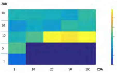
[image:4.595.53.288.80.185.2]While this result is interesting, it is necessary to understand how varying the parameters in the model will affect the songs produced by the population. To achieve this, we created a series of 500 experiments, in which we used linear descent to vary the size of the ZOR, ZOA, breeding grounds, and feeding grounds. We then carry out a pairwise subtraction of every agent’s transition ma-trix from each other. This allows us to see whether the agents have converged on the same transition matrix or if there is a large amount of variety in them. These results were then stored in a 100x5 matrix. Each column corre-sponded with the size of the ZOA, and every 25 rows corresponded with an increase in the ZOR. Within those 25 rows and column is every combination of feeding and breeding ground size. We then took the mode of every group of these cells. This resulted in the matrix seen in Figure 7.
Figure 7: This graph shows how varying the pa-rameters of the ZOR and the ZOA affects the be-haviour of the model. The darker colours corre-spond to model runs that converged on similar songs. The bright colours represent experiments where the population had dis-similar songs.
5. ADAPTING THE MODEL
As it stands, the model does not capture the full complex-ity observed in humpback whale song. While agents in our model do converge on a shared song in certain situa-tions, it does not present any change once every agent in the population has learned the song. Furthermore, first order transition matrices are not capable of capturing the hierarchical structure of humpback whale song. Despite this, our model is at a stage where it can be adapted for algorithmic composition. In this section, we describe the technical aspects of adapting our model. Following this, we move on to discuss adding a novelty method inspired by computational musicology.
5.1 Technical Considerations
Open Sound Control (OSC) [15] is a protocol used to transmit data between different audio software programs. This allows for the quick adaptation of our model to be used as a tool for composition. Using OSC, we can send data to and from our model in order to generate new mu-sical sequences in real time. This is achieved using the Max4Live API in Ableton Live[16,17], so that the com-poser may introduce new songs sequences to the popula-tion, and play them back in order to generate new musical variations, based on this input and other parameter set-tings. This is illustrated in Figure 8.
!
39!
!
Figure(17:(This(figure(shows(two(different(examples(of(the(scenario(1(group(sorting.(The(first(two(figures(on(the(top(row(show(the(movement(of(the(whales.(From(the(Levenshtein(distance(tree((third( figure(on(the(top(row),(we(can(see(that(the(agents(developed(an(identical(song.(In(the(bottom(three( figures(however,(we(can(see(that(the(agents(have(sorted(themselves(into(three(distinct(groups(with( three(different(songs.((
As!we!can!see!from!figure!17,!the!spatial!sorting!can!have!a!dramatic!effect!not!
only!on!the!different!groups!of!agents,!but!also!on!the!songs!that!they!have.!Fig.!
18!shows!these!agents!grammars!in!more!detail,!and!it’s!easy!to!see!that!they!
have!converged!on!a!very!simplistic,!unrealistic!grammar.!!
!
!
Figure(18:(The(grammar(of(our(twenty(agents(from(the(top(scenario.(This(gives(us(a(very(short( simple(song(of(the(form(of(([1,8,10,10](!
39!
!
Figure(17:(This(figure(shows(two(different(examples(of(the(scenario(1(group(sorting.(The(first(two( figures(on(the(top(row(show(the(movement(of(the(whales.(From(the(Levenshtein(distance(tree((third( figure(on(the(top(row),(we(can(see(that(the(agents(developed(an(identical(song.(In(the(bottom(three( figures(however,(we(can(see(that(the(agents(have(sorted(themselves(into(three(distinct(groups(with( three(different(songs.((
As!we!can!see!from!figure!17,!the!spatial!sorting!can!have!a!dramatic!effect!not!
only!on!the!different!groups!of!agents,!but!also!on!the!songs!that!they!have.!Fig.!
18!shows!these!agents!grammars!in!more!detail,!and!it’s!easy!to!see!that!they!
have!converged!on!a!very!simplistic,!unrealistic!grammar.!!
!
!
Figure(18:(The(grammar(of(our(twenty(agents(from(the(top(scenario.(This(gives(us(a(very(short( simple(song(of(the(form(of(([1,8,10,10](
[image:4.595.58.281.291.389.2]Figure 8: Signal flow from Ableton to the model.
[image:5.595.56.282.324.386.2]In order to interact with the model, the user uses the ComposerIn device with a MIDI keyboard to create a sequence of notes and rhythms to be learned by a selected agent in the model. These notes are appended to a list in Max/MSP, where they are then formatted so that they can be used as an input to the model. The sequence is then sent via OSC to the selected agent, who estimates a first order transition matrix so that it may create variations on this theme. This interaction flow is demonstrated in fig-ure 9.
Figure 9: This shows how a composer interacts with the model.
At each iteration of our model, the song produced by each agent is sent back to Ableton Live using the modelOut device, where they are transposed in order for them to be formatted into MIDI notes. These are then stored in a message box and sequenced using a metro object. This allows the MIDI notes to be sent to any Live or Max4Live device that the composer wishes to use.
5.2 The Need for Novelty
Since the model relies on the distance between agents to influence the transmission of the song, it is possible for the song input by the composer to be overpowered by the other songs in the population of agents. This leads us to add a new dimension to the model, which will allow the user to interact with the model and actually observe the impact of their input. To achieve this, the model is ex-tended to have a new bias added; novelty. Chosen due to theories that is a factor in humpback song evolution. [9]
Originally, we took inspiration from the work of Todd, [18] where novelty is determined by the built in expectations of the agents. This was used to develop in equation 5.
α= ! !"# (!!! )!!!(!(!),!(!!!))
! (5)
Given a sequence, S, which is indexed using the value n,
an agent calculates novelty, α, based on its transition matrix, T. N, the number of elements in the sequence S, is used as a weighting. This is defined by equation 5. The square brackets indicate that an absolute value should be taken for the top term of the equation. This novelty value,
α, is used to update our learning algorithm, as shown in equation 6.
𝑇!= 𝐴∗(1−𝐼∗α) +(𝐵∗ 𝐼∗α ) (6)
The novelty bias has a significant impact on what songs our agents choose to learn from. Low novelty will result in a song having no impact on the transition matrix of a listening agent, while a high novelty value will lead to that songs estimated transition matrix almost completely taking over the listening agent’s transition matrix (Figure 10).
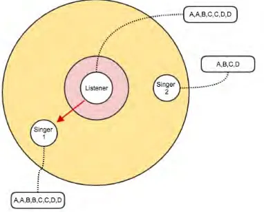
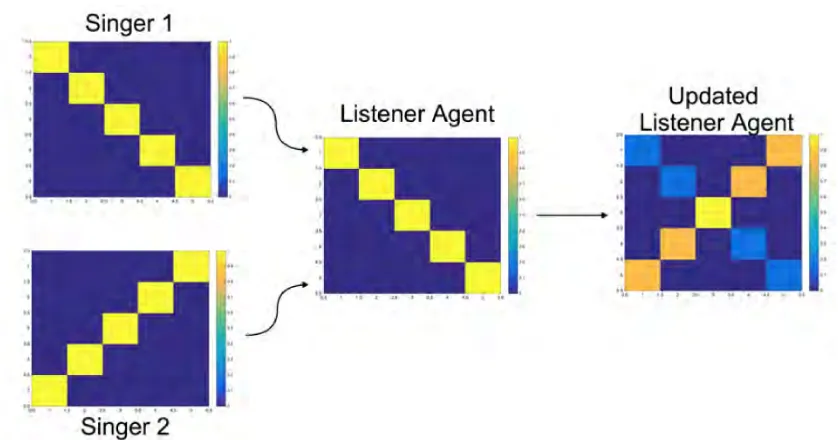
Figure 10: How the novelty algorithm affects a listener agent's transition matrix. Singer 1 and 2 are both equidistant from the listener agent. The listener learns more of singers 2 song since it is more novel in comparison to its own transition matrix.
278
[image:5.595.71.490.526.746.2]The results returned from this method are interesting, but we found that the transition matrices in a population would converge to uniform distribution. Rather than our novelty value being weighted by the number of elements in a sequence, we have our novelty value weighted by the agent that has the highest novelty value.
nov[m]= !max (𝑇 𝑆(𝑛 )−𝑇(𝑆(𝑛),𝑆(𝑛+1))
! (7)
α=!"#!"#!!!" (8)
We also introduce a learning rate with this algorithm, which is scaled between 0 and 1. This updates our agents learning algorithm to the following, seen in equation 13.
𝑇!= 𝐴∗(1−𝐼∗(α∗LR) +(𝐵∗(𝐼∗(α∗LR)) (9)
[image:6.595.310.539.166.286.2]The dynamic weighting algorithm produces an oscillating effect on the probability of transitioning from one unit to another, as demonstrated in Figure 11. This shows the probability of an agent moving from unit A to unit B (the red line), and the probability of moving from unit A to unit C (the blue line). At the start of the model, the prob-ability of going from unit A to B is 100%. Another agent in the population is trained with a probability of transfer-ring from unit A to C 100% of the time. As our agents meet on the breeding grounds they hear the song, they hear this new song and deem it to be more novel than their own, thus applying more emphasis to learning it.
Figure 11: The figure demonstrates how the dynamic novelty algorithm creates an oscillation in the proba-bility of transitioning from one unit to the other. (Transitioning from unit 1 to 2 in blue, transitioning from unit 1 to 3 in red).
6. MUSICAL DEMO
In order to test the model, we approached it from a com-positional point of view. First, four different musical themes were chosen to form the structure of the composi-tion. These themes were chosen specifically because they have a high novelty value when compared to each other.
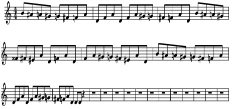
[image:6.595.55.272.427.592.2]They are also easily recognisable rudimentary musical features. They consist of an ascending C major arpeggio (Theme A), a descending chromatic scale (Theme B), an ascending D minor arpeggio (Theme C), and a repeating G# (Theme D). These themes can be seen in figure 12. At the start of our composition, every agent’s transition ma-trix is trained by theme A. We then presented all subse-quent themes to only a single agent (agent 2). We then recorded the songs being produced by agent 1 via MIDI.
Figure 12: The four themes used in the composition. The resulting composition is interesting, as the oscillatory nature described in section 5.2 of this document emerged not only for simple transitions as was originally observed, but also for the structured themes presented to our popu-lation. Whenever a new theme was introduced, the agent would move between the two themes, before the entire population would settle on some form of hybrid theme. We called this theme oscillation (figure 14). The corre-sponding hybrid theme is shown in figure 13. This is demonstrated at the point where each transition is intro-duced.
Figure 13: An example of a hybrid theme.
Figure 14: An example of theme oscillation.
7. CONCLUSION AND FUTURE WORK
From this paper, we have seen that scientific methods for the analysis of animal vocalisations may easily be adapted for algorithmic composition. Here, we demon-strated the model as a stand alone scientific tool, [image:6.595.308.539.545.654.2]plained the technical considerations necessary for user interaction, and developed a novelty method that allows a user to have a direct impact on the songs in the popula-tion. Emergent properties, such as theme oscillation and hybrid themes were also demonstrated through a compo-sitional demo. Future work will involve exploring the parameter space described in section 4, to investigate how it may be used as a tool to influence the emergence of hybrid themes seen in this model. It is also necessary to carry out a full investigation of the impact that the novelty metric has on the evolution of songs in the popu-lation. Finally, a method of song innovation must be pro-duced. Although our agents develop interesting hybrid songs, they do not have any in built mechanism for song evolution. The use of the model to develop rhythmic themes is also an area that would warrant further investi-gation.
Acknowledgments
The authors wish to thank The Leverhulme Trust for funding this project.
8. REFERENCES
[1] S. Kirby, “Spontaneous evolution of linguistic structure - An iterated learning model of the emergence of regularity and irregularity,” IEEE Trans. Evol. Comput., vol. 5, no. 2, pp. 102–110, 2001.
[2] H. Whitehead, P. J. Richerson, and R. Boyd, “Cultural Selection and Genetic Diversity in Humans,” Selection, vol. 3, pp. 115–125, 2002.
[3] C. Hartman and B. Beneš, “Autonomous boids,” in Computer Animation and Virtual Worlds, 2006, vol. 17, no. 3–4, pp. 199–206.
[4] E. R. Miranda, S. Kirby, and P. Todd, “On Computational Models of the Evolution of Music: From the Origins of Musical Taste to the Emergence of Grammars,” Contemporary Music Review, vol. 22, no. 3. pp. 91–111, 2003.
[5] E. R. Martins, Joao M., Miranda, “Engineering - The Role of Social Pressure: A New Artificial Life Approach to Software for Generative Music,” i-managers J. Softw. Eng., vol. 2, no. 3, 2008.
[6] E. R. Miranda, Ed., A-Life for Music: Music and Computer Models of Living Systems. Middleton, Wisconson: A-R Editions, Inc., 2011.
[7] R. S. Payne and S. McVay, “Songs of humpback whales.,” Science, vol. 173, no. 3997, pp. 585– 597, 1971.
[8] R. Payne, K., Tyack, P., & Payne, “Progressive changes in the songs of humpback whales (Megaptera novaeangliae): A detailed analysis of two seasons in hawaii,” in Communication and Behavior of Whales, no. 9–57, 1983, pp. 9–57.
[9] C. Noad, Michael J., Cato, Douglas H., Bryden, M. M., Micheline, Jenner, Jenner, “Cultural Revolution in Whale Songs,” Nature, vol. 408, no. 537, 2000.
[10] E. C. Garland, A. W. Goldizen, M. L. Rekdahl, R. Constantine, C. Garrigue, N. D. Hauser, M. M. Poole, J. Robbins, and M. J. Noad, “Dynamic horizontal cultural transmission of humpback whale song at the ocean basin scale,” Curr. Biol., vol. 21, no. 8, pp. 687–691, 2011.
[11] P. Jones, Eric and Oliphant, T. and Peterson, “SciPy: Open Source Scientific Tools for Python.” 2001.
[12] A. Kirke, S. Freeman, E. Miranda, and S. Ingram, “Application of Multi-Agent Whale Modelling to an Interactive Saxophone and Whales Duet,” in
Proceedings of International Computer Music Conference, 2011, no. August, pp. 350–353. [13] A. Kirke, E. Miranda, L. Rendell, and S. Ingram,
“Towards Modelling Song Propagation in Humpback Whales,” in Proceedings of 2015 Conference on Transdisciplinary Approaches to Cognitive Innovation, 2015.
[14] J. D. Darling, M. E. Jones, and C. P. Nicklin, “Humpback whale songs : Do they organize males during the breeding season ?,” Behaviour, vol. 9, no. 143, pp. 1051–1101, 2006.
[15] M. Freed, Adrian, and Wright, “Open Sound Control.” Centre for New Music and Audio Technologies.
[16] “MAX/MSP.” Cycling 74.
[17] “Live.” Ableton.
[18] P. M. Todd and G. M. Werner, Frankensteinian Methods for Evolutionary Music Composition. Cambridge, MA: MIT Press/Bradford Books, 1999.
280