Evaluating Methods for Short to Medium Term County Population Forecasting ESRI WP143(?) 2002

Evaluating Methods for Short to Medium Term

County Population Forecasting

By

Edgar Morgenroth

Economic and Social research Institute

Subsequently published as "Evaluating Methods for Short to Medium Term County Population Forecasting", Journal of the Statistical and Social Inquiry Society of Ireland, Vol. 31, pp.111-143, 2001/2002.

Abstract: Public services provision and land use planning are crucially

dependent on accurate population forecasts. Despite their importance,

particularly for planning at the local level, population forecasts for Irish

counties are not readily available. A number of different methods could be

used to calculate such forecasts, but it is not clear which of these possible

methods produces the most accurate forecasts. This paper assesses the data

requirements and methodology involved in the implementation of the various

techniques, and evaluates the forecasting performance of a number of

different methods in terms of the forecast error associated with each method

over the period 1991 to 1996. The results of this paper show that simple share

extrapolation techniques perform well compared with the more elaborate

cohort component model that is widely used for national projections.

Evaluating Methods for Short to Medium Term

County Population Forecasting

1. Introduction

Public services provision and land use planning are crucially dependent on accurate population forecasts. Such forecasts are particularly important at the local (county) level where they should determine planning decisions such as the provision of water and sewerage facilities, schools, hospitals etc. As such one would expect such forecasts to be produced on a regular basis and be readily available. However, this is not the case and rigorous county population projections are produced rarely and only for a few counties (e.g. Morgenroth, 2001, Brady Shipman Martin, 1999). In contrast national forecasts are produced regularly by the CSO (Central Statistics Office, 1988, 1995, 1999) and more recently the CSO has published regional projections (Central Statistics Office, 2001).

One factor which may have prevented the production of county level projections is the choice of the appropriate method that should be applied. A number of different methods could be used to calculate such forecasts. These include, trend extrapolation methods, the life table/cohort component method, time series modelling and econometric modelling. It is, however, not clear which of these possible methods produces the most accurate forecasts. Furthermore, issues of ease of implementation and data requirements of these methods have not been examined in the Irish context.

error particularly if the forecast horizon is very long. As a result it is not advisable to project to far into the future and hence the focus of this paper is on the short to medium term. Nevertheless, the forecasting methods tend to use current trends which assume no significant changes to policy. Thus, if major policy changes occur the outcome regarding population is likely to be different than that predicted.

This paper will outline in detail the data requirements and methodology involved in the implementation of the various techniques, and will then evaluate the forecasting performance of the different methods in terms of the forecast error associated with each method when applied to projecting county populations from 1991 to 1996. In doing so the paper will for the first time apply such a large set of techniques to forecast Irish county population. Crucially it will provide a more comprehensive evaluation of the various methods than has hitherto been available, since other papers on the evaluation of population forecasts have used a more restrictive set of methods (e.g. Smith, 1987), or were conducted in relation to population forecasts of larger spatial units (e.g. Smith and Sinicich, 1992). This paper is thus not concerned with explaining historical population trends for Irish counties which was the subject of a paper by Walsh (2000), neither is it concerned with a detailed evaluation of recent trends in fertility or migration (see Fahey and Russel, 2001 on fertility and Punch and Finneran, 1999, Barrett, 1999 or Fitz Gerald and Kearney, 1999, on migration).

2. Alternative Projection Methods

There are many methods that can be used to generate population projections at the county level. These include the well known cohort component method, simple extrapolation methods, regression based extrapolation, correlated indicators, time series methods (ARIMA), and structural econometric models. Here the focus will be on all bar the latter two methods, since the time series methods require a long time series of equal periodicity and preferably at a high frequency which is not available for Irish counties1. Furthermore, the construction of a structural econometric model of Irish county populations which would incorporate internal and external migration and fertility is beyond the scope of this paper.

2.1. Cohort Component/Life Table

At the national level the most widely used projection method is probably the cohort component/life table method. This involves disaggregating the Census data by cohort and then moving these cohorts along their life cycle. Thus, deaths are subtracted from each cohort according to mortality rates from the life table. The mortality rates can be adjusted for expected improvement in life expectancy. Births are calculated on the basis of age specific fertility rates and these are subject to infant mortality. Finally, assumptions need to be made about migration, both internal and external2. This method is thus based on the fundamental balancing equation of population growth which defines population growth as the result of births minus deaths plus net migration for each county which is defined as follows:

) (

)

( _{i i i i}

i B D I E

g = − + − (1)

where g_i denotes the increase in the population of county i, B_idenotes the

number of births in the county, D_idenotes the number of deaths in the county,

i

I denotes the number of immigrants into the county and E_idenotes the number of emigrants out of the county. The first term in parenthesis thus defines the natural increase of the population and the second term in parenthesis defines net migration into the county. Clearly the latter incorporates both internal migration in the country and external migration to and from other countries.

The population at a particular point in time, say period 1, is thus equal to the population in the base period 0 plus the net increase in the population between the base period and period 1:

i i

i P g

P₁ = ₀ + (2)

Projections are then constructed by assuming or estimating numbers of births deaths and migration.

Thus, this method is intuitive and deals with the basic factors that determine the size of the population. However, the drawback of this method is that it requires strong assumptions regarding fertility, mortality and migration. The latter are particularly difficult at the regional and county level. Furthermore, while dealing with these issues they are not accounted for in a behavioural model. On the other hand this method yields detailed results not only of the total size of the population but also of the gender balance, age balance, number of deaths and number of births.

2.2. Simple Trend Extrapolation

to project the population forward, assuming that this trend is stable up to the projection horizon. Clearly this again is a strong assumption which may not hold in practice, particularly if developments take place that cause a structural break in the evolution of the population e.g. an economic crisis that leads to large scale emigration.

In order to outline these techniques it is useful to first define the relevant variables that are used. The projected total population is denoted P_if, where i

denotes the county. In order to identify the trend data is required for two points in time between which the trend is measured. This period is denoted the base period which covers y years and the projection horizon covers x years. At the start of the base period a population P_i0 is observed and at then end of this

period a population P_i1is observed. Using these two variables the average annual growth rate between the start and the finish of the base period, r can be calculated. Using this notation two simple extrapolation techniques, namely linear (LINE) and exponential (EXPO) extrapolation, can be defined as follows.

Method 1 linear extrapolation (LINE)

(

)

1 i i

i

if _y P P

x P

P = + − (3)

Method 2 exponential extrapolation (EXPO)

( )

P

P_if = _i1exp (4)

population at the start of the base period isPS₀ and the total national population

at the end of the base period is denotedPS₁. The simple share extrapolation method (SHARE) is then given as:

Method 3 shares of state population (SHARE)

            − + = 0 0 1 1 1 1 PS P PS P y x PS P PS

P i i i

f

if (5)

The techniques described in this section are distinct from the cohort component/life table methods that are commonly used for national projections. The advantage of these simpler trend methods is that they require less data which makes them particularly suitable for population projection at a spatially disaggregated level for which data for some variables required for the cohort component method may not be available. Furthermore, they are easily implemented yielding quick results. The disadvantage of these methods is that they use past trends to predict the future whereas the cohort component model tracks individual cohorts on the basis of an assumed life expectancy.

2.3. Regression Based Extrapolation

A method that is closely related to the simple trend extrapolation methods described above is that of regression based share extrapolation (see for example Cantanese, 1972 and Klosterman, 1993). The distinguishing feature of this technique is that the projected share is generated using regression techniques which are applied to more than two data points. The use of these regression techniques results in a smoothing out of the estimated trend.

which fits best, say according to the _R2_{, is chosen. Of course there are many}

possible functional forms, including non-linear ones (see Cantanese, 1972 and Klosterman, 1993 for examples). Here the focus is on functional forms that are either linear or that can be linearised. Specifically, the simple linear model, the power function/log-linear model and the exponential model are used. Adding a constant to the relationship described above, these are given as:

1. Linear

T

S_i =α +β (6)

2. Log Linear (power function)

β

αT

S_i = (7)

which can be linearised by taking logs to yield the following:

T S_i log

log =α +β (8)

Exponential

T i

S =αβ (9)

which can again be linearised by taking logs to yield the following:

T S_i log (log )

log = α + β (10)

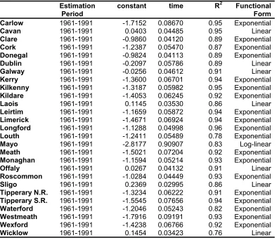
2.4. Correlated Indicators (Electoral Register)

The final method considered here uses data other than the Census data in order to apportion changes in the population. The main criterion for choosing such variables is that they must be highly correlated with the total population. For example, the electoral register that is updated annually can be used to estimate the population. In order to implement this method a similar approach to the regression based share extrapolation method can be used. However, this is applied to the ratio of people on the electoral register to the number of persons in the county, at the census dates. This ratio is then regressed on time, using the three functional forms outlined above. Again the functional form is chosen according to best fit and the parameters of this estimation are then used to project the ratio of electors to the population at a point in time. Then the population at that point in time can be estimated if the number of persons on the electoral register is known. This means that this method can not be used to project the population to a future date but this method may nevertheless prove useful in providing estimates of the population in the intercensal period or before census figures are available. Of course a lagged version of this method could be employed to provide actual forecasts, but this would require the estimation of a time series model with lags which is not feasible with the available data since the periodicity is not constant.

Again using this approach requires strong assumptions which may not hold in practice. However this method can be applied with relative ease and it has the added advantage that it can be extended to relate population movements to any variable that is thought to be highly correlated with population.

3. Data, Assumptions and Calculations

assumptions that are needed to construct the projections will be outlined and the projections will be generated.

Since the trend extrapolation methods are the simpler methods it is useful to start with these. They merely require data on county populations for at least two years in the case of the simple methods and for more than two years in the case of regression based techniques. This data can be easily obtained from the Census of Population, which has been carried out in Ireland since 1841. The last census preceding 1996 for which the projections are to be calculated was in 1991. It is then straightforward to estimate the trend in the case of the simple techniques. Of course a choice has to be made regarding the starting point for the base period. The obvious choice is 1986 so that the trend is estimated over the 5 year intercensal period that immediately precedes the projection period. However, one may also take the view that a longer term trend might reflect better the evolution of the population so that 1981 could also be used as the start for the base period.

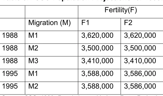
The SHARE and regression based techniques also require national level population projections from which the county populations can be obtained once predicted population shares have been constructed. Here, two possible sets of projections are available, namely the CSO projections published in 1988 and those published in 1995 (see CSO 1988 and CSO 1995). In each case a number of different projections are put forward by the CSO reflecting different migration and fertility assumptions which are denoted by M and F. These are shown in Table 3.1.

Table 3.1 CSO Population Projections for 1996. Fertility(F)

Migration (M) F1 F2

1988 M1 3,620,000 3,620,000

1988 M2 3,500,000 3,500,000

1988 M3 3,410,000 3,410,000

1995 M1 3,588,000 3,586,000

1995 M2 3,588,000 3,586,000

Source: CSO, 1988: Population and Labour Force Projection: 1991 – 2021, and CSO, 1995: Population and Labour Force Projection: 1996 – 2026.

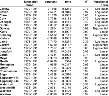
An important decision regarding the regression based share extrapolation method is the choice of time period over which to estimate the time trend. On the one hand a minimum number of observations is required for estimation, while on the other hand going back too far in time may give rise to estimates of the trend that bear no relationship with recent trends. The period that was chosen for the estimation was 1979 to 1991 (just 4 observations) which resulted in a good fit in most cases. However, for a few counties a slightly longer sample period was required to achieve a reasonable fit of the estimated relationship.

The results of the regression for the best fitting functional form for each county are reported in Table 7.1. The table shows that in most cases the fit of the regression equation is extremely good. It also shows that no one functional form dominates in terms of best fit, which justifies the use of the three different functional forms. Furthermore, the estimated coefficients show that these differ quite substantially, with some counties having a positive trend while others have negative trend in the share of the national population.

applied using data from 1961 to 1991. This is used to generate the ratio of electors to the population for each census year over that period. This ratio has been rising, reflecting the changing age structure of the Irish population. The regression results of the best fitting method are shown in Table 7.2. Again the fit is generally very good indicating that the estimated relationships have a high within sample forecasting accuracy. Also notable is the positive estimated trend for all counties.

births are subject to an infant mortality rate which is calculated at 7.60651011 per 1000 births4. Also it is assumed that 51.4% of births are male5.

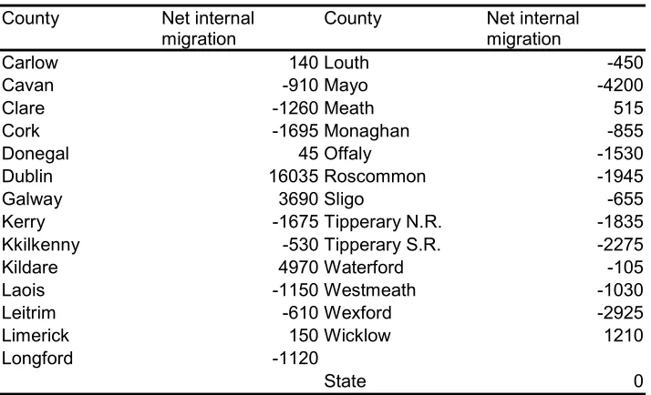
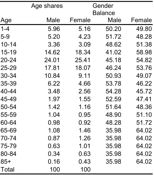
Finally, assumptions have to be made regarding migration, both internal and external. This is the most difficult aspect of the cohort component methodology since migration flows are influenced by economic conditions both at home and abroad, changes in attitude, and changes in policy which are not known in advance. These issues are particularly important for county population forecasting since an outflow of a relatively small number of people due to migration can be quite significant as a percentage of the total population in that county. With regard to internal migration figures are available from the census, in that it records the number of persons who were resident in a different county one year previous, which allows net internal migration to be estimated for each county for a one year period. In the absence of other research that might suggests the trend in these migration figures it is convenient to assume that these absolute numbers are constant over the following 5 year period and these are set out in Table 7.46. In order to generate the age and gender breakdown of these internal migration figures age and gender shares were applied. While these do vary between counties, for simplicity it was decided to apply the average national rates to all counties. While this might impact on the age and gender specific numbers it will not impact on the total number of persons which is the relevant number for the comparison in projection performance that will be carried out below.

The issue of international migration is more difficult to deal with. While both Hughes and Walsh (1980) and Sexton, Walsh, Hannan and McMahon (1991) deal with international migration at the county level which they derive from figures

contained in the Census, these refer to earlier periods. Nevertheless, in the absence of other information the pattern of international migration that was estimated for the 1981 to 1986 period by Sexton, Walsh, Hannan and McMahon (1991) is used here. This pattern is applied to the migration assumptions used by the CSO in making their population projections (CSO, 1988) which are set out in Table 7.3. The total numbers of net international migration are then allocated according to the shares derived from Sexton, Walsh, Hannan and McMahon (1991). Thus, some counties experience net international immigration while most experience emigration. Furthermore, following the CSO assumptions, migration is equally split between males and females and in terms of age distribution that assumed by the CSO is applied.

Clearly the assumption regarding internal and particularly international migration are important but unlikely to represent the actual pattern of migration over the period 1991-1996. Therefore, another migration assumption is added namely that there is no net international migration (M0).

4. Projections and Comparison of Projection Performance

Having dealt with the derivation and data requirements for the different methods in the previous chapter this chapter outlines the estimation results and deals with the main objective of this paper, that is the comparison of these with the actual population as enumerated by the 1996 Census of Population and to identify which is the most accurate method.

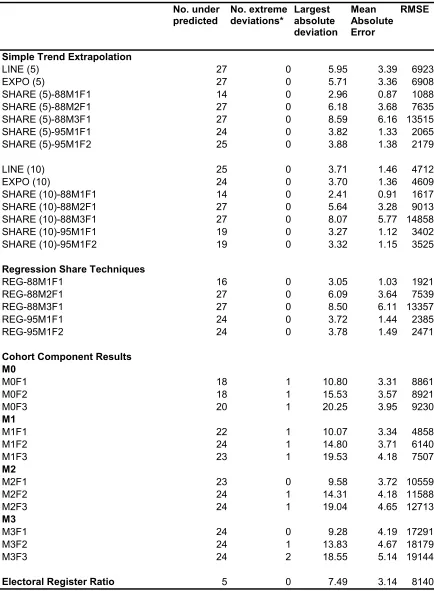
However, while it is clear that the predictions are not perfect and in most cases below the actual population of 1996, a more formal evaluation of the predictive performance of the different methods is needed. In order to accomplish this a number of measures are calculated. First, in order to identify whether a particular method is biased towards under or over predicting, the number of counties for which each method under predicts is counted. Secondly, the number of extreme deviations, that is deviation of more than 10% from the actual figure recorded in 1996 are shown in the third column of that table. Clearly, if a method gives rise to many such extreme observations its results should be only cautiously used since, if used for planning purposes, such deviating projections could lead to a substantial misallocation of resources. The third measure, the largest absolute deviation, also refers to this type of deviation. Fourthly, the mean absolute deviation is a useful measure of the average accuracy of each projection method, as is the root means squared error (RMSE).

These indicators of predictive performance are found in Table 4.1. The first column of that table confirms that most methods underpredict in the majority of cases, with the exception of the correlated indicators (electoral register) method that overpredicts in a majority of cases. The second column provides important information in that only the cohort component method yields extreme deviations, which is also confirmed by the third column which shows that these deviations are as large as 20%. The simpler methods perform considerably better in this regard with the best performance achieved by the simple share method using 1988 M1F1 national projections. In this case the largest deviation is just under 3%.

Table 4.1 Measures of Projection Performance No. under predicted No. extreme deviations* Largest absolute deviation Mean Absolute Error RMSE

Simple Trend Extrapolation

LINE (5) 27 0 5.95 3.39 6923

EXPO (5) 27 0 5.71 3.36 6908

SHARE (5)-88M1F1 14 0 2.96 0.87 1088

SHARE (5)-88M2F1 27 0 6.18 3.68 7635

SHARE (5)-88M3F1 27 0 8.59 6.16 13515

SHARE (5)-95M1F1 24 0 3.82 1.33 2065

SHARE (5)-95M1F2 25 0 3.88 1.38 2179

LINE (10) 25 0 3.71 1.46 4712

EXPO (10) 24 0 3.70 1.36 4609

SHARE (10)-88M1F1 14 0 2.41 0.91 1617

SHARE (10)-88M2F1 27 0 5.64 3.28 9013

SHARE (10)-88M3F1 27 0 8.07 5.77 14858

SHARE (10)-95M1F1 19 0 3.27 1.12 3402

SHARE (10)-95M1F2 19 0 3.32 1.15 3525

Regression Share Techniques

REG-88M1F1 16 0 3.05 1.03 1921

REG-88M2F1 27 0 6.09 3.64 7539

REG-88M3F1 27 0 8.50 6.11 13357

REG-95M1F1 24 0 3.72 1.44 2385

REG-95M1F2 24 0 3.78 1.49 2471

Cohort Component Results M0

M0F1 18 1 10.80 3.31 8861

M0F2 18 1 15.53 3.57 8921

M0F3 20 1 20.25 3.95 9230

M1

M1F1 22 1 10.07 3.34 4858

M1F2 24 1 14.80 3.71 6140

M1F3 23 1 19.53 4.18 7507

M2

M2F1 23 0 9.58 3.72 10559

M2F2 24 1 14.31 4.18 11588

M2F3 24 1 19.04 4.65 12713

M3

M3F1 24 0 9.28 4.19 17291

M3F2 24 1 13.83 4.67 18179

M3F3 24 2 18.55 5.14 19144

5. Projections for 2001 and 2006

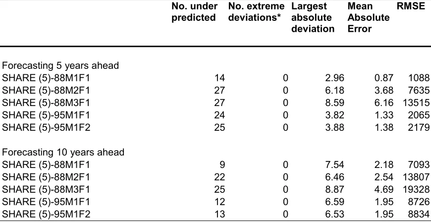
Having established the most accurate projection method, it is interesting to use this to produce real projections for the period from the last census (1996). Keeping with the 5-year intercensal interval a 5-year projection involves the production of projections to 2001, which has of course passed. Thus, it is of more relevance to increase the projection horizon to 10 years, which of course increases the forecast error dramatically. The national projections that were published by the CSO in 1999 are used along with the SHARE method that performed best. Since it is not clear at this stage which of the projections provided by the CSO are the most accurate the whole set of projections is again used. The results are shown in Table 7.8.

Since these figures may be used for planning purposes a brief comparison with the CSO projections of regional populations are in order (see CSO 2001). A number of interesting differences emerge. For example the results contained in this paper regarding the Dublin population are lower in all cases compared to the CSO projections. Overall these projections are larger then the CSO projections for the Mid-West, South-West, Mid-East, Border, Midlands and West regions but lower for Dublin and the South-East. They are therefore suggesting a somewhat different pattern of population change, with regions such as the Midlands not doing as badly as predicted by the CSO.

than that for 1986 to 1991, keeping the total national projections as before. The table clearly shows the increase in the forecast error, in terms of the largest absolute deviation, the mean absolute error and root mean squared error (RMSE). This simple analysis implies that the projections for 2006 need to be interpreted cautiously.

Table 5.1 Measures of Prediction Accuracy using the SHARE method to predict the 1996 county populations with for 5 and 10 year projection horizons

No. under

predicted No. extremedeviations* Largestabsolute deviation

Mean Absolute Error

RMSE

Forecasting 5 years ahead

SHARE (5)-88M1F1 14 0 2.96 0.87 1088

SHARE (5)-88M2F1 27 0 6.18 3.68 7635

SHARE (5)-88M3F1 27 0 8.59 6.16 13515

SHARE (5)-95M1F1 24 0 3.82 1.33 2065

SHARE (5)-95M1F2 25 0 3.88 1.38 2179

Forecasting 10 years ahead

SHARE (5)-88M1F1 9 0 7.54 2.18 7093

SHARE (5)-88M2F1 22 0 6.46 2.54 13807

SHARE (5)-88M3F1 25 0 8.87 4.69 19328

SHARE (5)-95M1F1 12 0 6.59 1.95 8726

SHARE (5)-95M1F2 13 0 6.53 1.95 8834

6. Conclusion

This paper has outlined a number of different population projection methods, and has applied these to predict the population for each county in 1996 in order to evaluate the predictive performance of each of these methods. These methods include the familiar cohort component method, simple extrapolation techniques, regression based share extrapolation and a correlated indicator method.

attributed to the assumptions made in deriving the cohort component results. However, assumptions need to be made in each method and it will not be known ex-ante which set of assumptions is correct, so that a researcher will always be faced with difficult choices regarding these assumptions. Furthermore, for the share extrapolation methods the assumptions are simple and do not require much research. The results found here, also concord with those found by Swanson and Beck (1994) which found particularly large absolute deviations for the cohort component method (up to 57%).

It should be noted that none of the methods considered here explicitly incorporate policy variables that will have important effects on the population distribution within the country, migration decision and fertility. Incorporating these would require a structural modelling approach, which would capture the effect of policy on migration and fertility and which could, apart from prediction, could also be used to evaluate the effect of policies.

7. Appendix

Table 7.1 Regression Results for the Regression Based Share Extrapolation (REG)

Estimation

Period constant time R

2 _Functional

Form Carlow 1979-1991 -0.1865 0.1214 0.77 Log-linear

Cavan 1979-1991 2.5761 -0.7846 0.97 Log-linear

Clare 1979-1991 0.1379 0.2933 0.83 Log-linear

Cork 1979-1991 2.7758 -0.1163 0.79 Log-linear

Donegal 1966-1991 1.6850 -0.1441 0.40 Log-linear

Dublin 1966-1991 2.6352 0.2685 0.61 Log-linear

Galway 1979-1991 1.2804 0.0219 0.98 Exponential

Kerry 1979-1991 5.0694 -0.1007 0.99 Linear

Kilkenny 1979-1991 0.5102 0.0141 0.96 Exponential

Kildare 1979-1991 -4.3448 0.4902 0.99 Linear

Laois 1971-1991 0.7470 -0.1271 0.35 Log-linear

Leirtim 1979-1991 1.5039 -0.1147 0.99 Exponential

Limerick 1979-1991 1.7857 -0.0162 0.86 Exponential

Longford 1979-1991 1.5642 -0.0439 0.98 Linear

Louth 1971-1991 0.4234 0.1908 0.74 Log-linear

Mayo 1979-1991 6.3073 -0.1977 0.99 Linear

Meath 1979-1991 -2.6426 1.3514 0.95 Log-linear

Monaghan 1979-1991 1.9645 -0.0317 0.95 Linear

Offaly 1979-1991 2.1904 -0.0329 0.88 Linear

Roscommon 1979-1991 3.2482 -0.1107 0.99 Linear

Sligo 1979-1991 2.4658 -0.0570 0.99 Linear

Tipperary N.R. 1979-1991 2.4312 -0.6981 0.99 Log-linear

Tipperary S.R. 1979-1991 3.5607 -0.0896 0.99 Linear

Waterford 1966-1991 0.7131 0.0868 0.34 Log-linear

Westmeath 1971-1991 2.0381 -0.0170 0.60 Linear

Wexford 1979-1991 0.6714 0.1420 0.80 Log-linear

Table 7.2 Regression Results for the Correlated Indicators Extrapolation Estimation

Period

constant time R2 _Functional

Form Carlow 1961-1991 -1.7152 0.08670 0.95 Exponential

Cavan 1961-1991 0.0403 0.04485 0.95 Linear

Clare 1961-1991 -0.9860 0.04120 0.89 Exponential

Cork 1961-1991 -1.2387 0.05470 0.87 Exponential

Donegal 1961-1991 -0.9824 0.04113 0.89 Exponential

Dublin 1961-1991 -0.2097 0.05786 0.89 Linear

Galway 1961-1991 -0.0256 0.04612 0.91 Linear

Kerry 1961-1991 -1.3600 0.06701 0.94 Exponential

Kilkenny 1961-1991 -1.3187 0.05982 0.95 Exponential

Kildare 1961-1991 -1.4053 0.06245 0.92 Exponential

Laois 1961-1991 0.1145 0.03530 0.86 Linear

Leirtim 1961-1991 -1.1659 0.05872 0.94 Exponential

Limerick 1961-1991 -1.4671 0.06924 0.94 Exponential

Longford 1961-1991 -1.1288 0.04998 0.96 Exponential

Louth 1961-1991 -1.2411 0.05489 0.78 Exponential

Mayo 1961-1991 -2.8177 0.90907 0.83 Log-linear

Meath 1961-1991 -1.5021 0.07204 0.92 Exponential

Monaghan 1961-1991 -1.1594 0.05214 0.93 Exponential

Offaly 1961-1991 0.0267 0.04132 0.91 Linear

Roscommon 1961-1991 -1.0284 0.04449 0.93 Exponential

Sligo 1961-1991 0.2369 0.02995 0.86 Linear

Tipperary N.R. 1961-1991 -1.3234 0.06222 0.91 Exponential

Tipperary S.R. 1961-1991 -1.5545 0.07656 0.94 Exponential

Waterford 1961-1991 -1.2046 0.05243 0.82 Exponential

Westmeath 1961-1991 -1.7916 0.09191 0.93 Exponential

Wexford 1961-1991 -1.4238 0.06766 0.92 Exponential

Wicklow 1961-1991 0.1454 0.03423 0.76 Linear

Table 7.3 Assumed Net International Migration for the State, 1991-1996

Cohort M0 M1 M2 M3

0-4 0 0 -2000 -4000

5-9 0 0 -2000 -4000

10-14 0 0 -2000 -2000

15-19 0 -14000 -24000 -34000 20-24 0 -50000 -70000 -80000 25-29 0 -18000 -24000 -38000 30-34 0 2000 -4000 -12000

35-39 0 0 -2000 -6000

40-44 0 0 0 0

45-49 0 0 0 0

50-54 0 0 0 0

55-59 0 0 0 0

60-64 0 0 0 0

65-69 0 5000 5000 5000

70-74 0 0 0 0

75-79 0 0 0 0

80-84 0 0 0 0

85+ 0 0 0 0

Total 0 -75000 -125000 -175000 Note: M0 indicates zero net migration. The other numbers were taken from CSO, 1988: Population and Labour Force Projection: 1991 – 2021, Table J.

Table 7.4 Assumed Net Internal Migration 1991-1996

County Net internal

migration County Net internalmigration

Carlow 140 Louth -450

Cavan -910 Mayo -4200

Clare -1260 Meath 515

Cork -1695 Monaghan -855

Donegal 45 Offaly -1530

Dublin 16035 Roscommon -1945

Galway 3690 Sligo -655

Kerry -1675 Tipperary N.R. -1835

Kkilkenny -530 Tipperary S.R. -2275

Kildare 4970 Waterford -105

Laois -1150 Westmeath -1030

Leitrim -610 Wexford -2925

Limerick 150 Wicklow 1210

Longford -1120

Table 7.5 Assumed Age and Gender Breakdown for Internal Migration, 1991-1996

Age shares Gender Balance

Age Male Female Male Female 1-4 5.96 5.16 50.20 49.80 5-9 5.20 4.23 51.72 48.28 10-14 3.36 3.09 48.62 51.38 15-19 14.62 18.34 41.02 58.98 20-24 24.01 25.41 45.18 54.82 25-29 17.81 18.07 46.24 53.76 30-34 10.84 9.11 50.93 49.07 35-39 6.22 4.66 53.78 46.22 40-44 3.48 2.56 54.28 45.72 45-49 1.97 1.55 52.59 47.41 50-54 1.42 1.16 51.64 48.36 55-59 1.04 0.95 48.90 51.10 60-64 0.98 0.92 48.28 51.72 65-69 1.08 1.46 35.98 64.02 70-74 0.87 1.26 35.98 64.02 75-79 0.63 1.01 35.98 64.02 80-84 0.34 0.63 35.98 64.02 85+ 0.16 0.43 35.98 64.02

Total 100 100

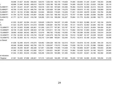
Table 7.6 County Population Projections for 1996 derived using Simple and Regression Based Trend Extrapolation and Correlated Indicators Methods

Carlow Cavan Clare Cork Donegal Dublin Galway Kerry Kilkenny Kildare Laois Leitrim Limerick Longford

Actual 1996 41,616 52,944 94,006 420,510 129,994 1,058,264 188,854 126,130 75,336 134,992 52,945 25,057 165,042 30,166

5 year trend

LINE (5) 40,896 51,627 90,492 408,003 126,570 1,029,159 182,176 119,629 74,084 129,065 51,344 23,567 159,343 29,096

EXPO (5) 40,896 51,640 90,493 408,010 126,579 1,029,166 182,185 119,650 74,085 129,235 51,353 23,625 159,364 29,119

SHARE (5)-88M1F1 42,167 53,241 93,307 420,700 130,516 1,061,100 187,820 123,365 76,382 133,019 52,948 24,314 164,316 30,010

SHARE (5)-88M2F1 40,769 51,476 90,214 406,754 126,189 1,025,926 181,594 119,276 73,850 128,610 51,192 23,508 158,869 29,016

SHARE (5)-88M3F1 39,721 50,153 87,894 396,294 122,944 999,545 176,925 116,209 71,951 125,303 49,876 22,904 154,784 28,269

SHARE (5)-95M1F1 41,794 52,770 92,482 416,981 129,362 1,051,720 186,160 122,275 75,707 131,844 52,480 24,099 162,864 29,745

SHARE (5)-95M1F2 41,771 52,741 92,431 416,748 129,290 1,051,134 186,056 122,207 75,664 131,770 52,450 24,086 162,773 29,728

10 year trend

LINE (10) 41,503 52,267 92,594 414,321 129,620 1,036,374 184,537 121,456 75,050 131,923 52,886 24,147 162,104 29,874

EXPO (10) 41,523 52,279 92,674 414,418 129,665 1,036,681 184,793 121,460 75,121 134,073 52,902 24,265 162,104 29,888

SHARE (10)-88M1F1 42,124 53,003 93,995 420,461 131,550 1,051,777 187,361 123,197 76,187 134,173 53,672 24,454 164,454 30,291

SHARE (10)-88M2F1 40,728 51,246 90,879 406,523 127,189 1,016,911 181,150 119,113 73,662 129,725 51,893 23,643 159,003 29,287

SHARE (10)-88M3F1 39,680 49,928 88,542 396,070 123,919 990,762 176,492 116,050 71,768 126,389 50,558 23,035 154,914 28,534

SHARE (10)-95M1F1 41,752 52,535 93,164 416,744 130,387 1,042,479 185,704 122,108 75,514 132,987 53,197 24,238 163,001 30,023

SHARE (10)-95M1F2 41,729 52,505 93,112 416,512 130,315 1,041,898 185,601 122,040 75,472 132,913 53,168 24,224 162,910 30,006

Regression Based

88M1F1 41,936 52,395 93,915 416,574 129,462 1,064,329 185,729 122,515 75,531 134,616 53,140 24,395 164,124 30,212

88M2F1 40,546 50,658 90,802 402,765 125,170 1,029,047 179,572 118,454 73,028 130,153 51,378 23,586 158,683 29,211

88M3F1 39,503 49,355 88,467 392,408 121,951 1,002,586 174,955 115,408 71,150 126,806 50,057 22,980 154,603 28,460

95M1F1 41,565 51,932 93,085 412,892 128,317 1,054,921 184,087 121,432 74,864 133,426 52,670 24,180 162,673 29,945

95M1F2 41,542 51,903 93,033 412,662 128,246 1,054,333 183,985 121,365 74,822 133,351 52,641 24,166 162,582 29,929

Correlated indicators

Table 7.6 continued.

Louth Mayo Meath Monaghan Offaly Roscommon Sligo Tipperary

N.R

Tipperary S.R

Waterford Westmeath Wexford Wicklow State

Actual 1996 92,166 111,524 109,732 51,313 59,117 51,975 55,821 58,021 75,514 94,680 63,314 104,371 102,683 3,626,087

5 year trend

LINE (5) 89,638 106,242 106,859 50,207 57,153 49,202 53,466 56,186 72,739 92,097 60,381 101,586 99,988 3,510,795

EXPO (5) 89,644 106,331 106,870 50,218 57,168 49,271 53,481 56,210 72,770 92,098 60,399 101,587 100,026 3,510,827

SHARE (5)-88M1F1 92,432 109,581 110,166 51,776 58,940 50,754 55,138 57,946 75,018 94,954 62,270 104,746 103,071 3,620,000

SHARE (5)-88M2F1 89,368 105,949 106,514 50,060 56,986 49,072 53,310 56,025 72,531 91,807 60,206 101,274 99,654 3,500,000

SHARE (5)-88M3F1 87,070 103,225 103,775 48,773 55,521 47,810 51,940 54,585 70,666 89,446 58,658 98,670 97,092 3,410,000

SHARE (5)-95M1F1 91,615 108,613 109,192 51,319 58,419 50,305 54,651 57,434 74,355 94,115 61,719 103,820 102,160 3,588,000

SHARE (5)-95M1F2 91,564 108,552 109,131 51,290 58,387 50,277 54,620 57,402 74,313 94,062 61,685 103,763 102,103 3,586,000

10 year trend

LINE (10) 91,829 108,687 110,346 51,344 58,585 50,574 54,397 57,289 74,239 93,141 62,059 103,563 102,173 3,566,876

EXPO (10) 91,864 108,775 111,010 51,344 58,585 50,653 54,403 57,302 74,254 93,206 62,060 103,620 102,880 3,568,113

SHARE (10)-88M1F1 93,198 110,184 112,125 52,088 59,436 51,257 55,171 58,097 75,288 94,544 62,963 105,116 103,832 3,620,000

SHARE (10)-88M2F1 90,109 106,532 108,408 50,362 57,466 49,558 53,342 56,171 72,792 91,410 60,876 101,632 100,390 3,500,000

SHARE (10)-88M3F1 87,792 103,793 105,621 49,067 55,988 48,284 51,970 54,727 70,920 89,059 59,310 99,019 97,809 3,410,000

SHARE (10)-95M1F1 92,374 109,210 111,134 51,628 58,911 50,804 54,683 57,584 74,622 93,708 62,406 104,187 102,914 3,588,000

SHARE (10)-95M1F2 92,323 109,150 111,072 51,599 58,878 50,776 54,653 57,551 74,581 93,656 62,372 104,129 102,857 3,586,000

Regression Based

88M1F1 93,759 109,509 113,076 51,846 59,241 51,115 54,837 57,776 74,889 93,580 63,182 104,757 103,558 3,620,000

88M2F1 90,651 105,879 109,328 50,127 57,277 49,421 53,019 55,861 72,407 90,478 61,088 101,284 100,125 3,500,000

88M3F1 88,320 103,156 106,517 48,838 55,805 48,150 51,656 54,424 70,545 88,152 59,517 98,680 97,551 3,410,000

95M1F1 92,930 108,541 112,077 51,388 58,717 50,663 54,352 57,265 74,227 92,753 62,624 103,831 102,643 3,588,000

95M1F2 92,878 108,480 112,014 51,359 58,685 50,635 54,322 57,233 74,186 92,701 62,589 103,773 102,585 3,586,000

Correlated indicators

Table 7.7 County Population Projections for 1996 derived using the Cohort Component Method (various assumption)

Carlow Cavan Clare Cork Donegal Dublin Galway Kerry Kilkenny Kildare Laois Leitrim Limerick Longford

Actual 1996 41,616 52,944 94,006 420,510 129,994 1,058,264 188,854 126,130 75,336 134,992 52,945 25,057 165,042 30,166

M1 F1 42,130 52,203 89,846 412,589 131,808 1,045,289 188,139 119,858 71,280 148,584 51,231 24,137 161,267 28,807

M1 F2 41,752 51,921 89,297 410,395 131,023 1,042,319 187,151 119,238 70,541 154,967 51,053 24,019 160,729 28,749

M1 F3 41,375 51,638 88,748 408,201 130,239 1,039,350 186,164 118,618 69,802 161,350 50,875 23,901 160,190 28,691

M2 F1 41,670 52,378 89,539 408,505 132,362 1,009,260 185,577 119,800 70,741 147,928 51,036 24,263 157,064 28,885

M2 F2 41,292 52,095 88,990 406,311 131,578 1,006,291 184,589 119,180 70,002 154,311 50,858 24,145 156,526 28,826

M2 F3 40,915 51,813 88,441 404,117 130,793 1,003,321 183,601 118,559 69,263 160,694 50,680 24,027 155,987 28,768

M3 F1 41,210 52,552 89,232 404,422 132,917 973,231 183,014 119,742 70,201 147,272 50,842 24,388 152,861 28,962

M3 F2 40,832 52,270 88,683 402,227 132,132 970,262 182,026 119,122 69,462 153,655 50,664 24,270 152,323 28,904

M3 F3 40,455 51,987 88,134 400,033 131,348 967,292 181,039 118,501 68,723 160,038 50,486 24,153 151,784 28,846

Louth Mayo Meath Monaghan Offaly Roscommon Sligo Tipperary

N.R

Tipperary S.R

Waterford Westmeath Wexford Wicklow State

Actual 1996 92,166 111,524 109,732 51,313 59,117 51,975 55,821 58,021 75,514 94,680 63,314 104,371 102,683 3,626,087

M1 F1 92,476 104,684 109,955 50,334 57,207 48,730 53,483 55,449 70,436 92,920 60,621 100,967 104,114 3,568,544

M1 F2 92,076 104,233 109,385 50,028 56,863 48,582 53,160 56,823 70,019 92,536 60,219 100,610 103,682 3,561,371

M1 F3 91,677 103,781 108,814 49,723 56,534 48,434 52,838 58,197 69,602 92,153 59,816 100,253 103,250 3,554,212

M2 F1 92,279 105,559 109,581 50,161 57,368 49,072 52,879 55,272 69,473 92,107 59,810 101,625 104,351 3,518,544

M2 F2 91,880 105,108 109,010 49,856 57,025 48,924 52,556 56,646 69,056 91,724 59,407 101,267 103,919 3,511,371

M2 F3 91,480 104,656 108,440 49,550 56,696 48,776 52,234 58,019 68,639 91,341 59,005 100,910 103,487 3,504,212

M3 F1 92,082 106,434 109,207 49,989 57,530 49,414 52,275 55,095 68,510 91,294 58,999 102,282 104,588 3,468,544

M3 F2 91,683 105,983 108,636 49,683 57,186 49,266 51,952 56,468 68,093 90,911 58,596 101,925 104,156 3,461,371

Table 7.8 Predicted Population for the years 2001 and 2006 calculated using the SHARE method and CSO national predictions

Carlow Cavan Clare Cork Donegal Dublin Galway Kerry Kilkenny Kildare Laois Leitrim Limerick Longford

2001

M1F1 43,505 54,576 99,977 443,223 135,647 1,123,517 203,336 134,242 79,279 152,163 55,102 25,487 172,984 30,862

M1F2 43,482 54,547 99,925 442,992 135,576 1,122,931 203,230 134,172 79,238 152,084 55,073 25,474 172,893 30,846

M1F3 43,482 54,547 99,925 442,992 135,576 1,122,931 203,230 134,172 79,238 152,084 55,073 25,474 172,893 30,846

M2F1 43,222 54,220 99,325 440,334 134,763 1,116,195 202,011 133,367 78,762 151,171 54,743 25,321 171,856 30,661

M2F2 43,188 54,177 99,247 439,988 134,657 1,115,316 201,852 133,262 78,700 151,052 54,700 25,301 171,721 30,637

M2F2 43,188 54,177 99,247 439,988 134,657 1,115,316 201,852 133,262 78,700 151,052 54,700 25,301 171,721 30,637

2006

M1F1 45,406 56,134 106,165 466,458 141,307 1,190,996 218,536 142,657 83,302 170,614 57,246 25,845 181,020 31,491

M1F2 45,170 55,844 105,615 464,040 140,574 1,184,824 217,403 141,918 82,870 169,730 56,949 25,711 180,082 31,328

M1F3 45,036 55,677 105,300 462,659 140,156 1,181,297 216,756 141,495 82,623 169,225 56,779 25,635 179,546 31,235

M2F1 44,487 54,998 104,016 457,018 138,447 1,166,894 214,113 139,770 81,616 167,161 56,087 25,322 177,357 30,854

M2F2 44,263 54,721 103,492 454,716 137,750 1,161,016 213,035 139,066 81,205 166,319 55,805 25,195 176,464 30,698

M2F3 44,128 54,555 103,178 453,335 137,331 1,157,489 212,387 138,643 80,958 165,814 55,635 25,118 175,928 30,605

Louth Mayo Meath Monaghan Offaly Roscommon Sligo Tipperary

N.R.

Tipperary S.R.

Waterford Westmeath Wexford Wicklow State

2001

M1F1 96,295 115,504 117,526 52,760 61,437 53,503 58,530 59,814 78,260 100,635 66,633 109,774 111,430 3,836,000

M1F2 96,245 115,444 117,464 52,732 61,405 53,476 58,500 59,783 78,219 100,582 66,598 109,717 111,372 3,834,000

M1F3 96,245 115,444 117,464 52,732 61,405 53,476 58,500 59,783 78,219 100,582 66,598 109,717 111,372 3,834,000

M2F1 95,667 114,751 116,760 52,416 61,036 53,155 58,149 59,424 77,750 99,979 66,198 109,059 110,704 3,811,000

M2F2 95,592 114,661 116,668 52,375 60,988 53,113 58,103 59,378 77,689 99,900 66,146 108,973 110,616 3,808,000

M2F2 95,592 114,661 116,668 52,375 60,988 53,113 58,103 59,378 77,689 99,900 66,146 108,973 110,616 3,808,000

2006

M1F1 100,442 119,392 125,666 54,121 63,732 54,952 61,274 61,528 80,949 106,802 70,019 115,281 120,665 4,052,000

M1F2 99,922 118,773 125,014 53,841 63,401 54,668 60,957 61,210 80,530 106,248 69,656 114,684 120,039 4,031,000

M1F3 99,624 118,420 124,642 53,681 63,213 54,505 60,775 61,027 80,290 105,932 69,448 114,342 119,682 4,019,000

8. References

Barrett, A. (1999). “Irish Migration: Characteristics, Cause and Consequences”.

IZA Discussion Paper No. 97. Bonn: Institute for the Study of Labour.

Brady Shipman Martin, Kirk KcClure Morton, Fitzpatrick Associates and Colin Buchanan and Partners, (1999). Strategic Planning Guidelines for the

Greater Dublin Area, Dublin: Department of the Environment and Local

Government.

Cantanese, A. (1972). Scientific Methods of Urban Analysis. Aylesbury: Leonard Hill Books.

Central Statistics Office (1988). Population and Labour Force Projection: 1991 – 2021. Dublin: Stationery Office.

Central Statistics Office (1995). Population and Labour Force Projection: 1996 – 2026. Dublin: Stationery Office.

Central Statistics Office (1996a). Census 91, Volume 8 Usual Residence and

Migration. Dublin: Stationery Office.

Central Statistics Office (1996b). Report on Vital Statistics. Dublin: Stationery Office.

Central Statistics Office (1999). Population and Labour Force Projection: 2001 – 2031. Dublin: Stationery Office.

Central Statistics Office (2001). Regional Population Projections: 2001-2031. Statistical Release, Dublin: Central Statistics office.

Fahey, T., and H. Russell (2001). “Family Formation in Ireland: Trends, Data Needs and Implications. ESRI Policy Research Series Paper No. 43. Dublin: Economic and Social Research Institute.

Fitz Gerald, J., and I. Kearney (1999). “Migration and the Irish Labour Market”.

ESRI Working Paper No. 113. Dublin: Economic and Social Research

Institute.

Klosterman, R. E., Brail, R. K., E.G. Bossard, eds. (1993). Spreadsheet Models

for Urban and Regional Analysis. New Brunswick, N.J.: Center for Urban

Policy Research.

Morgenroth, E. (2001).“Analysis of the Economic, Employment and Social Profile of the Greater Dublin Region”. ESRI Books and Monographs Series Paper,

Dublin: Economic and Social Research Institute.

Punch, A., and C. Finneran (1999). “The Demographic and Socio-Economic Characteristics of Migrants, 1986-1996”. Journal of the Statistical and Social

Inquiry Society of Ireland. Vol. XXVII (1), pp.213-252.

Sexton, J.J., Walsh, B., Hannan, D., and D. McMahon (1991). “The Economic and Social Implications of Emigrations”. NESC Report No. 90. Dublin: National Economic and Social Council.

Smith, S. K. (1987). “Tests of Forecast Accuracy and Bias for County Population Projections. Journal of the American Statistical Association, Vol. 82, No. 400, pp.991-1012.

Smith, S. K. and T. Sinicich (1992). “Evaluating the Forecast Accuracy and Bias of Alternative Population Projections for States”. International Journal of

Forecasting. Vol. 8, pp. 495-508.

Svanson, D., and D. Beck (1994). “A New Short-Term County Population Projection Method”. Journal of Economic and Social Measurement, Vol. 20, pp. 25-50.