Analysis of Human Mobility Patterns from GPS Trajectories and Contextual Information
Katarzyna Siła-Nowicka1,4, Jan Vandrol2, Taylor Oshan3, Jed Long1, Urška Demšar1, A.
Stewart Fotheringham3
1
School of Geography & Geosciences, University of St Andrews, Scotland, UK
2
School of Energy, Environmental Technology and Agrifood, Cranfield University, UK
3
GeoDa Centre, School of Geographical Sciences and Urban Planning, Arizona State University, Tempe, Arizona, USA
4
Urban Big Data Centre, University of Glasgow, Scotland, UK
Abstract:
Human mobility is important for understanding the evolution of size and structure of urban
areas, the spatial distribution of facilities, and the provision of transportation services. Until
recently, exploring human mobility in detail was challenging because data collection methods
consisted of cumbersome manual travel surveys, space-time diaries or interviews. The
development of location-aware sensors has significantly altered the possibilities for acquiring
detailed data on human movements. While this has spurred many methodological
developments in identifying human movement patterns, many of these methods operate
solely from the analytical perspective and ignore the environmental context within which the
movement takes place. In this paper we attempt to widen this view and present an integrated
approach to the analysis of human mobility using a combination of volunteered GPS
trajectories and contextual spatial information. We propose a new framework for the
trajectory segmentation, data mining and spatio-temporal analysis. We are interested in
examining if and how travel modes depend on the residential location, age or gender of the
tracked individuals. Further, we explore theorised “third places”, which are spaces beyond
main locations (home/work) where individuals spend time to socialise. Can these places be
identified from GPS traces? We evaluate our framework using a collection of trajectories
from 205 volunteers linked to contextual spatial information on the types of places visited
and the transport routes they use. The result of this study is a contextually enriched data set
that supports new possibilities for modelling human movement behaviour.
Keywords: Movement analysis, trajectories, trajectory segmentation, travel mode
classification, significant places.
1. Introduction
Understanding human mobility is a major contributor to the development of knowledge on
important issues such as the form and function of urban areas, the location of facilities and
the demand for transportation services. Human mobility has traditionally been explored by
manual travel surveys, space-time diaries or interviews (Palmer et al. 2013), all of which are
time consuming, expensive and do not provide a sufficient spatio-temporal resolution to
allow the investigation of mobility patterns in detail. The development of sensors that capture
movement information in real time and at detailed spatial and temporal scales (e.g. GPS
trackers) has changed our ability to collect movement data (Kwan and Neutens 2014).
However, the developments in movement data collection technologies are much further ahead
than current methods for extracting meaningful patterns from such data (Laube et al 2007,
Long and Nelson 2013). While recently there have been several new methodological
data, many of these ignore the embedding of movement into the geographical context (Purves
et al. 2014). There is a need to investigate new ways to identify movement patterns
considering movement data not only on their own, but within their environmental context.
In this paper we approach this problem through an integrated analysis of human movement
from GPS trajectories linked to contextual information. Purves et al. (2014) list several
alternative definitions of context for movement data: 1) context identified from additional
data collected simultaneously with GPS trajectories, 2) context provided by the description of
space within which movement occurs and 3) context provided through knowledge about
physical/biological properties of the movement process. In this study we define context as
option 2); that is, the contextual data used in this study provide a description of the spaces
that people move through.
A particular characteristic of human movement is the variety of different travel modes via
which movement can take place. This is of particular interest in areas such as urban planning
(Schwanen and Moktharian 2005) because residential location-choice and travel-choice may
be interconnected. It is known that the built environment and the socio-demographic
characteristics of individuals have impacts on the choice of transportation mode for daily
travel such as commuting (Ewing and Cervero 2010). This impact is an extensively
researched topic in transportation geography and has traditionally been explored using data
from surveys and questionnaires (Van Vugt et al. 1996, Rodriguez and Joo 2004, Schwanen
and Moktharian 2005, Wener and Evans 2007). New research has involved using GPS
trajectories to identify transportation modes from raw data and annotate the original
trajectories with these modes to create semantic trajectories (Yan et al. 2013). Such semantic
al. 2010), navigation (Sester et al. 2012), privacy protection (Parent et al. 2013) and inferring
social structure from trajectory proximity (Xiao et al. 2014). There has, however, been little
or no connection between these two points of view. We offer an alternative where we identify
transportation mode from real GPS data while at the same time exploring if and how this
mode is affected by the residential location of our participants.
Patterns of human mobility are linked to how people influence their spatial context and how
the spatial context influences them in return (Palmer et al. 2013). A location becomes a place
through perceptions of it and the activities of the people who use it, which in turn affects the
behaviour of the people there. Thus, human movement is not only embedded into
geographical space, but can be considered as movement between places imbued with
meaning through human activities (Gieryn 2000). From the sociological perspective, each
individual moves through a set of hierarchically ordered places that have a particular meaning
for him/her (Oldenburg 1989). The most important place, termed the first place, is home,
where an individual spends most of his/her time. The second place is work or school or a
place where a major regular activity takes place. In the process of building social capital,
each individual also frequents so-called “third places”. These places are neither home nor
work-related and are places where people spend their leisure time and socialise with others.
They can include many different types of locations: shops, cafes, bars, libraries, bookshops
(Oldenburg 1989, Holm 2013) and have become a popular subject of study in sociology,
urban geography and retail geography (Holm 2013, Laing and Royle 2013, Lin 2012,
Steinkuehler and Williams 2006). However, to our knowledge, there have been no studies
investigating third places using empirical tracking data. There are a number of technological
studies that identify the so-called significant places from movement data (places where
2007), but these are not necessarily ‘third places’ and the studies are generally devoid of
context. For example, Bhattacharya et al. (2012) only use the geometrical properties of
movement inferred from GPS trajectories to identify significant places and purposely exclude
the geographical context (“instead of considering additional resources such as geometry of
Point Of Interests (POIs) or map matching techniques, to identify a place as significant, we propose a technique that automatically extracts all significant places and their corresponding durations” solely from users’ GPS trajectories (Bhattacharya et al. 2012,
p.399)). Umair et al. (2014) identify significant places from GPS data based on the spatial
density of GPS points in the neighbourhood of each location, again disregarding any
contextual information.
We propose to investigate movement from transportation and sociological points-of-view
using a novel framework to integrate trajectory data with contextual information. As Kwan
(2013) states, “people’s spatio-temporal experiences are influenced not only by where they
live, but also by other places they visit, when they visit these places, how much time they spend there, what they experience as they travel between these places”. To address these
different aspects of movement, we offer a new integrated approach that involves several
perspectives.
From the technological perspective we propose a new framework for identifying and
analysing dynamic (movement) and static (places) behaviour from trajectories and associated
contextual information. We do this through a combination of trajectory segmentation,
classification and spatio-temporal analysis using movement trajectories linked to contextual
spatial data. From the perspective of transportation geography we are interested in whether
tracked. From a sociological perspective we explore the existence of “third places”. We are
interested in the temporal dynamics and the spatial distribution of these places – as far as we
know this is the first attempt to use real movement data for this purpose. Further, we are
interested in how gender and age might affect movement patterns and report our results
segmented by these two characteristics. We evaluate our framework on a data set of GPS
trajectories from 205 volunteers in three Scottish towns who were continuously tracked in
their daily movements for a week. We enrich these trajectories with contextual information
from external sources to identify mobility patterns in the volunteers’ daily lives.
2. Related Work
The framework we employ consists of a combination of several analytical methods for
movement data: trajectory segmentation of raw data; identification of significant places; and
classification of behaviour (static behaviour - types of places and dynamic behaviour - travel
modes). In this section we review related work on these methods.
Segmentation is the process of dividing a movement trajectory into sub-trajectories called
segments, where each segment fulfils certain criteria (Buchin et al. 2011). Segmentation is
frequently derived using “movement parameters”, i.e. statistical properties of the movement
process at each trajectory point. These include velocity, speed, heading, acceleration, turning
angle, angular range, displacement, straightness index, sinuosity, tortuosity, and other locally
calculated features (Dodge et al. 2009, Dodge et al. 2012).
In transportation, a combination of segmentation and data mining is frequently used for the
classification of travel mode. Sester et al. (2012) identify important places to divide
trajectories into segments of constant travel mode. Torrens et al. (2011) use machine learning
(Self-Organising Maps) to classify different motion types. Zheng et al. (2010) use a change-point
segmentation method to classify GPS trajectories into travel modes.
Significant places (Liao et al. 2007) can be identified from GPS trajectories using clustering
or machine learning (Ye et al. 2009, Rodrigues et al. 2014, Umair et al. 2014). Studies
identifying significant places can be broadly categorised into two groups: those identifying
personally meaningful locations for individuals (Ashbrook and Starner 2003, Kang et al.
2004, Zhou et al. 2007, Bhattacharya et al. 2012) and those finding significant places for
multi-users that identify general places of interest (Ashbrook and Starner 2002, Agamennoni
et al. 2009, Zheng et al. 2009 and Yin et al. 2014). Some studies use check-in histories (Lian
and Xie 2011) or user similarity (Shaw et al. 2013) to identify attractive locations. Andrienko
et al. (2013) propose a visual analytics methodology for identifying significant places.
Important places have also been identified from mobile phone trajectories (Isaacsman et al.
2011).
It is also important to categorise the activity that occurred in each of these places. Zhou et al.
(2007) and Huang et al. (2013) classify activity places into major and minor places using the
time spent in each place and the frequency of an individual re-visiting a place. Liao et al.
(2007), Kang et al. (2004) and Zhou et al. (2007) assign the categories of ‘home’ or ‘work’ to
an activity place using ‘dwell-time’ as the main class separator. Our proposed framework
incorporates each of these steps: segmentation, travel mode classification and the
identification and categorisation of significant places.
To evaluate our proposed framework, we used data collected in a GPS travel survey and
external data sources describing the environment within which the movement occurred.
3.1. GPS travel survey
In 2013 we gathered mobility data from 205 participants living in the three largest towns in
the Kingdom (county) of Fife in Scotland: Dunfermline, Glenrothes, and Kirkcaldy. These
towns were selected due to their different socio-economic characteristics which we expected
would be reflected in the movement behaviour of their residents. Dunfermline (pop. 49,706)
is an old town located about 20km north of Edinburgh. A large proportion of the inhabitants
commute to Edinburgh for work, either by car or public transportation. Glenrothes (pop.
38,679) was established in the late 1940s as one of Scotland’s post WWII new towns and is
an industrial centre approximately half way (approx. 50km) between Edinburgh to the south
and Dundee to the north. Kirkcaldy (pop. 49,709) is an old town located 30km north east of
Edinburgh, across the Firth of Forth. It has a small medieval centre surrounded by 17th-19th
century developments and large areas of modern housing and industrial estates.
We designed our GPS survey to recruit volunteers of all ages and demographics. Many
contemporary movement studies use trajectories collected from social media (Twitter,
Foursquare), which creates an age bias towards the younger population (Bricka et al. 2012).
In order to counteract this bias, we decided to recruit participants using a traditional method:
by sending invitations via the mail to a randomly selected sample of participants. Further, we
wanted our sampling to represent the spatial distribution of inhabitants in the three towns so
that invitations were sent to a number of randomly selected addresses obtained from the
publically available Electoral Register of Scotland which were spatially distributed to reflect
smallest census unit in UK, while postcodes are even smaller spatial areas, widely used for
geocoding, but they are not a perfect subdivision of data zones.
A maximum response rate for a traditional household or travel survey in UK is held to be
around 60% (Anderson et al. 2009, Dunstan 2012). Out of these responders, at most 20%
could be expected to be willing to carry a GPS device and/or perform the travel survey
(Bonnel et al. 2009). This means that we could expect a maximum response rate of 12%; in
the end, however, we achieved only a 4% response rate. We sent 6,000 invitations, equally
divided between the three towns. Out of this, 252 (4.2%) volunteers responded positively and
upon being sent GPS trackers, 205 (3.4%) trackers were returned with usable data. The low
response rate probably reflects both the perceived technical nature of the data-gathering
process and the intrusion into people’s privacy.
In order to maximise the response rate and capture the widest possible audience, we did not
collect any personal information from the respondent, nor did we request a travel diary to be
completed. We expected to be able to compensate for the lack of extra information by using
open data from governmental sources, in particular the Electoral Register of Scotland. We
were able to obtain age information from this register although for some participants this
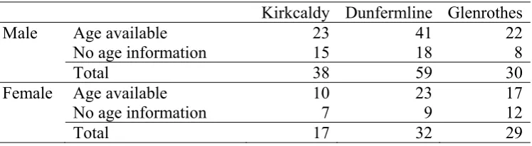
information was not publically available. Table 1 shows the breakdown of participants by
gender and location.
Table 1 somewhere here.
The participants were asked to carry GPS trackers continuously for a period of seven
which are equipped with motion sensors and were programmed to record the GPS location of
the individual every 5 seconds unless the device was in a stationary position for more than 2
minutes. Trajectories from all 205 participants in the main experiment comprise 3,869,831
raw GPS locations, where each location record consists of participant ID, latitude, longitude,
elevation, date and time. Figure 1 shows the spatial extent of collected trajectories.
Figure 1 somewhere here
Prior to the main data collection we also performed a pilot experiment, where volunteers
were tracked for a week. These pilot data1 were used to familiarise ourselves with the
operation of the trackers and were used as test data during the development of our
framework. The second aim of the pilot experiment was to determine the temporal sampling
rate: as per literature on GPS surveys we tested sampling rates of 1s (Krygsman and Nel
2009; Rasmussen et al. 2013), 5s (BMCT 2012), 10s (Marchal et al. 2008) and 30s (Itsubo
and Hato 2006). At the rate of 1s and tracking duration of one week, the pilot participants
collected on average 120000 GPS points, which exceeded the storage capacity of the tracker
(8Mb). A 5s sampling rate produced on average 19000 data points and filled 30% of the
storage capacity. Longer sampling rates (10s, 30s) produced data that were not accurate
enough to separate movement modes. As in similar studies (Bohte and Maat 2009), the
shortest sampling rate (1s) used up battery at a very fast rate. Based on these results from the
pilot experiment, we chose the 5s sampling rate for the main study, which had enough
accuracy for our purposes, did not drain the battery too quickly and did not exceed the
storage capacity of the tracker.
1
3.2. External Data
We expected that many participants would use public transport. Because of this, we obtained
the National Public Transport Access Node (NaPTAN) data (which contain locations of all
stations and stops of public transport) as an external source.
To be able to classify the types of significant places of individual participants, we used the
Point Of Interest data set for Scotland, produced by the Ordnance Survey UK (OS). These
data contain information about the locations of Points Of Interest, a hierarchical classification
of these (9 groups, 52 categories and 616 classes), the positional accuracy of the points and
the road network reference of the locations of each Point of Interest.
We augmented the OS Point Of Interest data by generating a supplementary Places Of
Interest data set through visual exploration of Google Maps and Openstreetmap. Note that
many Places of Interest are of an irregular size and shape (e.g. parking spaces and shopping
centres) and because of this they are better represented as polygons rather than points.
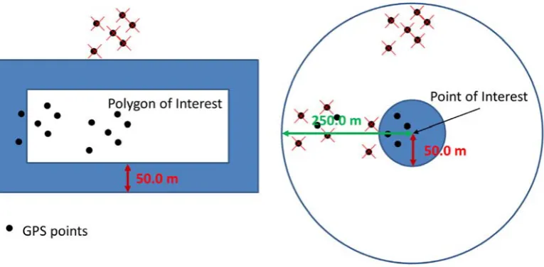
Matching a movement stop in the form of a segment of a GPS trajectory to a polygon
produces fewer errors than matching the segment to a point (fig. 2). We therefore created our
Places Of Interest as polygons rather than. We further digitised the OS Points Of Interest into
respective polygons and merged the two data sets. In the rest of the paper we refer to the
combined data of Points and Places of Interest as POI data.
The POI data consists of a set of different types of public spaces, such as shopping centres,
grocery shops, leisure centres, churches, hospitals, schools, etc. We grouped places into four
activity types as per table 2.
Table 2 somewhere here
4. Framework
The framework consists of three phases (fig. 3). The algorithms used in the framework are
provided as pseudocode in the Supplementary Online Material.
Figure 3 somewhere here
4.1. Phase One: Separating Dynamic and Static Behaviour
We consider the movement of one participant across the entire survey period as one
trajectory, which is partitioned into homogenous segments that correspond to different
movement modes. The partitioning process scans through trajectory points and when it
identifies a change in the spatio-temporal distribution of trajectory points, it creates a new
segment. For this, we define a new measure of the density of the logged positions in the
neighbourhood of each trajectory point, the Spatio-Temporal Kernel Window (STKW)
statistic. To calculate STKW values, we order all trajectory points by time. Then, for every
point we search in both directions along the trajectory and count the number of points within
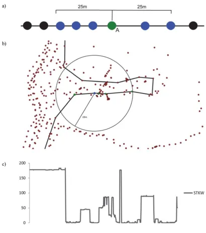
a specified threshold distance from the original point, A, in figure 4a. Our threshold distance
was set to 25m, which is sufficient to distinguish stops from slower (walk/run) and faster
movement modes (vehicle transport) considering the chosen sampling frequency (5Hz). As
soon as a point further away than the specified distance is encountered, the count in that
account points in the nearest neighbourhood that belong to other visits (fig. 4b). Figure 4c
shows changes in STKW for an example trajectory: these are very sudden when travel mode
changes, which allows us to identify breakpoints between segments.
Figure 4 somewhere here
To determine the start and end points of segments, the algorithm looks for maximal changes
in STKW values. It scans each trajectory using two moving windows - one facing backwards
and one forwards and then sums the STKW values within both windows. By comparing the
two sums, the algorithm decides if the point can be classified as a breakpoint between two
different travel modes. If the density of points (given by the STKW sum) on one side of the
current point is much higher than on the other side, then a point is designated as a breakpoint.
Sometimes the change in travel mode is more gradual and STKW builds up over several
points. To counter this, the algorithm searches through subsequent points for a point with the
greatest difference between the left and right STKW totals to become a new breakpoint.
Data collection was frequently temporarily halted and resumed at a later point in time from a
different location. This occurred for many reasons, including cold starts (i.e. a GPS tracker
needing to fix its current position before starting to collect data), movement inside buildings,
trackers running out of battery or being turned off by participants. Because of this, additional
breakpoints had to be introduced to split the segments into parts describing continuous
movement without temporal breaks. For this, when two temporally consecutive points within
a movement segment were located more than 280m apart from each other (maximum
distance that an object moving with 200km/h can cover within 5 seconds, which was the
breakpoints were ignored, thus eliminating outlying segments resulting from fake movements
when the tracker was taken indoors.
Finally, we classified segments into three movement mode categories (vehicle movement,
walk/running and a stop) using two movement parameters (Dodge et al. 2009): the median
speed and the median distance from the geometric centre of the segment. The tracker,
however, can still suggest movement when the person is stationary because of the nature of
GPS systems (e.g., multi-path effects, urban canyons, terrain obstructions). These errors can
produce high and low outliers and affect the calculation of the average speed. The median
speed therefore better represents the predominant speed throughout the segment. For this
reason, the second movement parameter, relevant for the identification of stops, is the median
distance of trajectory points in the segment from the geometric centre of the segment. Since
stop segments have their points clustered around one particular location, the median distance
from the geometric centre is able to separate them from segments representing movement.
Median distance is also less sensitive to outliers than are average distance or standard
deviation.
We used these two movement parameters to train a feed-forward neural network with back
propagation as a learning method (Haykin 2008). Neural networks are frequently used for the
classification of trajectory data due to their ability to deal with missing data and outliers
(Karlaftis and Vlahogianni 2011). Our neural network was composed of an input layer with
two neurons for each of the two movement parameters a hidden layer with three neurons and
an output layer with as many neurons as there were categories for the segment. We tested
several different configurations of the hidden layer, but found that the layer with three
Lower numbers of hidden neurons created a too generalised network which was unable to
classify border cases correctly. Initially we used one network to classify all types of classes
(movement classes and stop segments) and compared the results with the actual class of
objects in the training data set. This resulted in 13% misclassified objects. We therefore
re-designed the network to consist of two separate networks, one to separate stops from
movement and a second one to classify movement segments into walk/vehicle classes.
Resulting errors were 4% for stop/movement classification and 1% for walk/vehicle
classification. More details on this algorithm are provided in the Supplementary Online
Material.
The training set contained 250 manually classified segments and had an equal distribution of
classes. Once the network was trained, we used it to classify the remainder of the data set
comprising of 16789 individual segments. The results of this segmentation served as input in
the two consecutive phases, the analysis of places and the analysis of movement as shown in
figure 4.
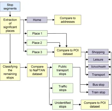
4.2. Phase Two: Analysis of Places
In the next step we identified the locations of significant places and categorise them
according to their importance by using external spatial data (fig. 5). Note that places are not
points, but are represented as stop segments, i.e. sub-trajectories.
Figure 5 somewhere here
To identify significant places, we calculate the frequency of re-occurrence and the amount of
a proxy for significance. The most frequently visited place with the longest total duration of
visits is considered to be home. Home locations derived in this way were compared to
addresses of participants in order to assess accuracy of our framework. We report on
accuracy in section 5.2. Theoretically, some individuals might spend more time in their place
of work or major daily activity (SP1) than at home. However, given the very high accuracy of
home identification (see section 5.2.) the potential for confusion between home and SP1 was
very small. An alternative possibility for home identification would be to identify places
where participants spend the night. However, as we base our classification on the sociological
theory of places (Oldenburg, 1989), we adopted the definition of home as the place where a
person spends most of his/her time. This also resolves theoretically possible issues of
participants who may spend nights at work and those who may live away from their partners
or families and spend certain nights at home and others at partner’s or family homes (e.g.
weekly commuters).
Home locations were excluded from further analysis, leaving us with a set of places that were
categorised using external contextual information. This process was based on the automatic
labelling of stop segments with information from our POI data set, which consisted of
polygons corresponding to interesting locations. All stops (sub-trajectories) found within the
proximity (50m buffer) of polygons representing the POIs (fig. 2) were assigned the activity
label based on the type of the POI (table 2).
The remaining uncategorised stops were compared to the NaPTAN database, described
above. If a stop was located in close proximity to a public transport stop, it was classified as
representing the corresponding mode of public transportation (waiting for bus/train). The
bus/train travel. The remaining stops were investigated for traffic patterns. In vehicle travel,
the movement is often interrupted with shorter stops, such as waiting at traffic lights or at the
entrance to a roundabout. We identified such traffic stops by selecting all stop segments that
were of less than 2 min duration and that occurred either between two segments previously
classified as vehicle movement or between a vehicle movement segment and a bus stop
(identified in the previous step). Further, if the transportation mode of the previous segment
were found to be a bus, the current stop and the following vehicle segments were reclassified
as bus travel. Stops that could not be identified through this procedure remained as
unidentified stops.
In order to investigate the existence of the “third places”, we used all stop segments (except
home) to identify the first three significant places (SP1, SP2 and SP3) for each participant.
These we defined as the three most frequently visited places with visits of longest duration
after home, while excluding places unsuitable for intentional socialising. This means that if a
place that fitted the definition of a significant place in terms of frequency and duration of
visits was a non-socialising place (e.g. a bus stop, a train station, a grocery store), it was
excluded from the set of significant places. Further, we limit ourselves to only three
significant places based on the longest duration of visits. These durations were on average of
212.6/48.5/18.4 min for SP1/SP2/SP3 on weekdays and 165.3/66.7/30.1 min for
SP1/SP2/SP3 on weekends. As SP4 had less than 5 min average duration for both weekends
and weekdays, it was considered too short to be included.
We expected that SP1 would be the location of either work or school (i.e. the location of the
main daily activity). However, since our participant sampling was voluntary, our
able to fully ascertain a matching between SP1 and work. Many such participants had leisure
places or shops as their SP1, which probably suggests respondents who are retired or have a
non-traditional working arrangement (e.g. working from home). We had no way of separating
these participants from those that worked in a particular location outside home (their SP1).
For this reason, we discuss SP1 together with SP2 and SP3.
4.3. Phase Three: Analysis of Movement
In the final phase we categorised the mode of transport on movement segments into
walking/running and vehicular movement, further subdivided into public transport and traffic
(fig. 3). The walking/running segments were already identified in the travel mode
classification. The vehicular movement was based on travel mode classification and the
identification of public transport and traffic stops. In the final step, consecutive segments of
the same category were merged and their attributes recalculated to reflect the newly formed
longer segments.
5. Results
We report results for the two steps: analysis of movement (travel mode classification) and
analysis of places (identification of stops).
5.1. Analysis of movement – travel mode classification
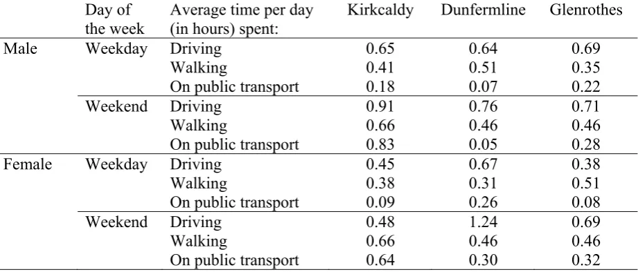
To prevent the identification of individuals or groups of individuals, we show all temporal
results as average times per day, broken down per weekdays and weekends as well as per
gender, and residential location. Table 3 shows the average time per day spent in each travel
mode. In general, there is more vehicle movement (both driving and public transport) during
note is a large increase in average time spent on public transport during the weekends
compared to weekdays for participants from Dunfermline which is in contrast to expectations
that public transport would be used primarily for commuting to work. We could not identify
any particular differences in the average use of travel modes between men and women.
Table 3 somewhere here
5.2. Analysis of places – identification and classification of stops
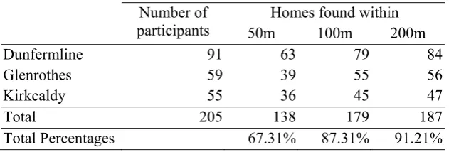
In order to estimate the accuracy of our place identification procedure, we compared the
centroids of home stops to the actual locations of the homes obtained from Openstreetmap
(OSM). Table 4 shows the results at spatial scales of 50, 100 and 200m with the highest
percentage of correct identification at 200m (91.21%), which demonstrates that we correctly
identify home locations within 200m in over 90% of the participants. This is comparable or
higher than similar studies: for example, Bohte and Maat (2009) report a 74% accuracy of
identifying homes from the GPS trajectories of 1104 people by extracting homes as ends of
trips. Liao et al. (2007) identify significant places with 90% accuracy although their sample
size was very small and included GPS trajectories of only four participants and their accuracy
assessment was undertaken for labelling (e.g. home, work, etc.) rather than for the locations
of places. Upon visually inspecting locations of some of the misclassified homes, we
speculate that the 90% accuracy was not an artefact of our data, but potentially related the
choice of OSM as the “ground truth” data. Geocoding street addresses is done in OSM by a
combination of actual points and interpolation, which leads to errors, as OSM automatically
excludes buildings of a certain size or type from its geocoding procedure (see Barron et al.
Table 4 somewhere here.
We calculated the average time per day spent at home per participant (fig. 6). Most
participants spent a reasonable amount of time at home (mostly between 10-16hrs) and most
people, as expected, stayed at home longer during the weekends than during weekdays (with
some exceptions, e.g. young females from Kirkcaldy).
Figure 6 somewhere here.
We also investigated the average times per day spent in SP1, SP2 and SP3, broken down by
weekdays and weekends (fig. 7). Interestingly, the participants spent a relatively large
amount of time in their SP1, regardless of the weekday/weekend split. SPs however are
individual and fixed for each person, that is, each participant has the same three SPs
regardless of the weekday/weekend break down. Since we are taking averages, it is not
possible to say if the same participants that spend on average a lot of time in their SP1 during
the week are the same participants that spend a lot of time there during the weekend.
Participants tend to spend more time in SPs 2 and 3 on weekends than on weekdays. Note
also women aged 60-69 from Glenrothes: their averages for SP1 and SP2 are similar for
weekdays and they spend a lot of time in their SP1 weekends, which might suggest that we
captured the pattern of retired people who do not go to work but spend their time in the same
locations regardless of the day of the week.
We were further interested in the spatial distribution of SP1, SP2 and SP3. Figures 10 and 11
show these distributions as kernel density estimates (KDE) for males and female participants
respectively. We used KDEs in order to prevent identification of individual participants. The
KDE maps have the cell size of 900m and use a 2000m radius in order to mask the exact
locations of individual travel while still providing a picture of the hotspots of the SP
distribution.
Figures 8 and 9 somewhere here
For Dunfermline we expected the SPs to be both within the town of Dunfermline and in the
city of Edinburgh. The first columns in figures 8 and 9 confirm this hypothesis for both men
and women. However, men have a more widespread spatial distribution of SPs in Edinburgh,
while women’s SP hotspots are limited to the centre. We speculate that this could be a
consequence of using public transport rather than driving. Most trains coming into Edinburgh
from the north via Fife only stop at the two main train stations in the centre of Edinburgh
(Haymarket and Waverley). Any participants taking these trains would therefore likely have
their SPs in the vicinity of these two stations. Of note also is a small cluster of men’s SP
hotspots in and around Glasgow (in the lower left corner of the maps in the first column of
fig. 9). These places are present through all levels, from SP1 to SP3 and most of them belong
to the same few participants. This is a common pattern: if one individual has a SP1 in a
certain location, it is likely that his/hers SP2 and SP3 will be in or near that same location.
Glenrothes participants were expected to have their SPs within the town as well as externally
around Fife. This is confirmed by patterns for both men and women (second column in figs. 8
Edinburgh and Fife towns (Kirkcaldy, Cupar and Dunfermline). There are also some
participants with SPs in Stirling (the hotspot near the westernmost point of the Firth of Forth)
and for men if SP1 is there (possibly indicating a place of work), SP2 and SP3 are also there.
For women, Stirling lacks a hotspot in SP1 distribution, suggesting that some female
participants travel to Stirling for leisure but do not work there.
Because of a lack of competing alternatives, Kirkcaldy residents were expected to have their
significant places mostly within the town. This is true to some extent for men and even more
for women (third columns in figs. 8 and 9).
Figure 10 somewhere here
To investigate the differences in spatial movement patterns further, we calculated the average
distance from home to SP1-2-3 respectively. Figure 10 shows radar plots of the average
distance broken down by residential location, gender and age. Home is in the centre of each
of these plots and the coloured lines show average distances for the three SPs for each age
group. Distances are up to a maximum of 50km from home. Given the total time spent at
home and in SP1, SP2 and SP3 we can consider a set of these four places together as a proxy
of an individual’s activity space. An activity space is a set of all areas within which an
individual has direct contact with others during his/her daily activities (Golledge and Stimson
1997). Considering our definition of SPs, it is likely that the first three together with home
approximate an activity space fairly well and this allows us to explore how these activity
spaces range in geographical size by age, location and gender. The results indicate some
In Kirkcaldy the activity spaces of females tend to be more circumscribed than those of males
whereas the opposite is the case in Glenrothes. In Dunfermline, the activity spaces of the two
genders are roughly the same in extent but vary in terms of the distances travelled to the
various SPs. Females travel further to their most common social destination than do males
but males travel much further to their second most common destination than do females. This
could either be due to females facing a greater scarcity of local employment and therefore
commuting to Edinburgh or fewer females being in the workforce and their most frequent
destination being Edinburgh for social trips. Without further contextual information it is
impossible to decide on the relative weights of these two explanations although the former
seems more likely given the frequency of the trips which suggests a daily pattern of travel.
The spatial extent of activity spaces also decreases with age, as in most cases these spaces are
very local for participants of ages 60-69. In Dunfermline and Kirkcaldy the most commonly
visited places for this age group are within a kilometre from home, while in Glenrothes they
are up to 2km away. This possibly reflects that retired participants socialise in their nearest
neighbourhood rather than travelling further away. The largest activity spaces are however
not limited to a particular age group or town. The three largest spaces belong to men of age
40-49 in Dunfermline (the distances are possibly related to SPs in Glasgow (fig. 8)), women
of age 20-29 in Glenrothes (distances relating to SPs in Stirling and Dundee (fig. 9)) and men
of age 50-59 in Kirkcaldy (distances relating to Stirling and Perth (fig. 8)). Given the
self-selecting sample of respondents and lack of contextual information it is not possible to
suggest any particular age-related interpretations of these spaces except for the likely
shrinking of activity spaces linked to retirement and old age.
In this paper we propose a framework combining movement analysis methods: segmentation,
analysing places, and identification of human mobility patterns (travel mode and places) from
a combination of volunteered GPS trajectories and contextual information. This work extends
previous studies by demonstrating a process for incorporating both movement-based and
place-based analysis into a single study to uncover new information about human movement
behaviour. We highlight how GPS tracking data can be utilised in conjunction with
contextual spatial information to study and understand individual travel behaviour and places
of interest. We highlight differences in behaviour based on residential location, gender and
age. While there are no particular differences in the use of travel mode between men and
women, our results suggest that the activity spaces of men are larger than those of women
and are larger for younger versus older adults.
This study also contributes to the literature documenting the “third places”. We develop a
methodology for capturing third places through the identification of typologically relevant
significant places (SPs) ordered by visit duration. As far as we know, this is the first attempt
to look for potential “third places” in GPS tracking data and represents a starting point for
future research into this area.
Although we highlight the potential of GPS traces for the identification of human mobility
patterns, the process is clearly not without difficulties. For instance, there are two types of
information that we decided not to include in our data collection in order to maximise the
response rate: demographic data and travel diaries. We expected that we would be able to
compensate for the lack of demographic information by accessing publicly available
governmental open data. However, since people can control the level of their personal
response rate was very low even without requesting such information and the balance has to
be struck between sample size and the amount of information requested from each volunteer.
An advantage of our data collection methodology compared to the collection of movement
data from social media (e.g. trajectories from Twitter, FourSquare), is that a relatively large
percentage of elderly participants (60+) were collected in our volunteer sample. This is in
contrast to assertion that GPS surveys are more likely to attract younger participants who are
probably more technologically knowledgeable than the elderly (Bricka et al. 2012). We
speculate that this might be due to the sense of inclusion: some elderly participants, who
perhaps are not comfortable with the current technological devices, may have felt that since
we made sure that the tracking task was a simple as possible, this was their one opportunity to
contribute to a technological experiment.
One of the recurring issues with the use of GPS traces for human mobility studies is the
noisiness of the trajectory data caused by the unpredictability of use of the trackers. In the
study it was assumed that participants would carry their trackers with them at all times, fully
charged and ready to track locations continuously. In practice, trackers occasionally lost
charge and were not re-charged and re-started until much later. Trackers were also taken to
unexpected locations such as destinations outside Scotland or used in unexpected travel
modes (there is a trajectory of a glider plane in our data, classified as vehicle travel by the
automatic algorithm!).
A further limitation are potential biases introduced by the short duration of the GPS survey
(one week). As we only tracked the participants over seven consecutive days, there is a
potential that we may not have captured the entire complexity of their daily movement and
vacation or could have experienced unusual events (emergencies or similar). Such
irregularities could introduce bias into our analysis and for individuals the frequency of visits
to places could therefore not necessarily correspond to their significance. Our solution to this
problem was to report aggregated results – the averages calculated for each group of
participants should have reduced this bias.
Another type of bias may also have been introduced with a relatively small sample size (205
individuals producing almost 4 million geocoded locations), which we tried to counter by a
relatively large number of invitations (6000) assuming a response rate of 12%. Having only
achieved a third of this response rate, this produced a smaller sample than anticipated. This
study should therefore be considered as a demonstrator for similar larger future studies rather
than providing absolute answers about movement behaviour of people in Fife.
A further issue that should be considered is the scalability of our framework to other cases
and in particular larger trajectory data sets. As trajectory analysis enters the Big Data era, it is
important that new frameworks and methods scale to increasingly larger data. Our data set is
a relatively small one and does not fit many of the characteristics of so-called Big Data (e.g.
volume, velocity, veracity, etc. (Kitchin 2013)), apart from being very fine-grained in its
resolution. Parts of the framework proposed here are based on knowing this data set very well
and it might be argued that the framework is somewhat bespoke. However, given that many
decisions performed during the development process are based on the general properties of
human movement (e.g. maximum possible velocities for driving a car, ranges accessible in
the sampling time period while moving at these velocities, the choice of movement
parameters used in neural network classification, etc.), this framework has a potential to scale
Finally, there is an enormous potential of using contextually enriched GPS trajectories to
investigate a range of important social phenomena. For example, if significant places are used
as a proxy for individuals’ activity spaces as we tentatively suggest, this knowledge could be
used to improve lives of residents by identifying locations where provisions of various types
of services are inadequate causing people to travel further to fulfil their social needs. SPs and
contextually enriched trajectories could also be used to delineate and define neighbourhoods,
the boundaries of which are often contested by residents. Another possibility would be to
investigate the temporal dynamics of spatial segregation. Spatial segregation is often linked
to inequality (Palmer et al. 2013); however this phenomenon is frequently only investigated
through residential census data which provides only a snapshot. Spatial and temporal
distribution of the use of SPs linked to information on class, race or ethnicity of participants
could provide a much more complex and dynamic picture of segregation, assisting not only
social scientists, but also policy makers and urban planners addressing inequality.
In conclusion, our study is only one of examples of analyses of real human movement data
that can and will become possible in the near future. These data are now becoming readily
available through both targeted data collection efforts such as ours or through pervasive
mobile devices. Further, as we demonstrate, GPS trajectories enriched with contextual spatial
information provide the potential to better understand and model human movement
behaviour. Our study is different from previous work (reviewed in section 2) in that it
combines approaches to movement analysis from three very different areas of research. We
integrate a technological methodology (GPS tracking) with spatial analysis approaches from
computer science and transportation geography as well as with theory from sociology. Such a
possible through the lens of a single discipline, thus opening new possibilities for the
empirical investigation of a range of social phenomena related to movement.
Acknowledgements
This work was supported by the EU FP7 Marie Curie ITN GEOCROWD grant
(FP7-PEOPLE-2010-ITN-264994). The authors would also like to thank all the survey participants.
References
Agamennoni, G, Nieto J, Nebot E, 2009 Mining GPS data for extracting significant places,
Robotics and Automation, 2009. ICRA '09. IEEE International Conference: 855-862
Anderson T, Abeywardana V, Wolf J and Lee M, 2009, National Travel Survey GPS
Feasibility Study, Department of Transport, UK.
Andrienko G, Andrienko N, Hurter C, Rinzivillo S and Wrobel S 2013 Scalable Analysis of
Movement Data for Extracting and Exploring Significant Places. IEEE Transactions in
Visualization and Computer Graphics 19(7):1078-1094
Ashbrook D and Starner T 2002 Learning Significant Locations and Predicting User
Movement With GPS, Proc. of 6th IEEE International Symposium on Wearable
Computing, Seattle, WA, 2002, 101-108
Ashbrook D and Starner T 2003 Using GPS to Learn Significant Locations and Predict
Movement across Multiple Users, Personal and Ubiquitous Computing 7: 275-286
Barron C, Neis P and Zipf A 2014 A Comprehensive Framework for Intrinsic
Beijing Municipal Committee of Transportation (BMCT) 2012 The fourth Beijing
comprehensive transportation survey report. Beijing Transport Research Centre,
Beijing Municipal Committee of Transportation.
Bhattacharya T, Kulik L and Bailey J 2012 Extracting significant places from mobile user
GPS trajectories: a bearing change based approach. Proceedings of the 20th
International Conference on Advances in Geographic Information Systems (SIGSPATIAL '12). ACM, New York, NY, USA, 398-401
Bohte W and Maat K 2009 Deriving and validating trip purposes and travel modes for
multi-day GPS-based travel surveys: A large-scale application in the Netherlands.
Transportation Research Part C: Emerging Technologies 17(3): 285-297
Bonnel P, Lee-Gosselin M, Zmud J and Madre J-L 2009 Transport survey methods: Keeping
up with a changing world. Emerald Group Publishing, Bingley, UK.
Bricka SG, Sen S, Paleti R and Bhat CR 2012 An Analysis of the Factors Influencing
Differences in Survey-Reported and GPS-Recorded Trips. Transportation Research
Part C, 21(1):67-88
Buchin M, Driemel A van Kreveld M and Sacristan V 2011 Segmenting trajectories: A
framework and algorithms using spatiotemporal criteria. Journal of Spatial Information
Science 3: 33–63
Dodge S, Weibel R and Forootan E 2009 Revealing the physics of movement: Comparing the
similarity of movement characteristics of different types of moving objects. Computers,
Environment and Urban Systems 33: 419–434
Dodge S, Laube P and Weibel R 2012 Movement similarity assessment using symbolic
representation of trajectories. International Journal of Geographical Information
Dunstan S, 2012, General Lifestyle Survey, Technical Appendices, Office for National
Statistics, UK.
Ewing R and Cervero R 2010 Travel and the Built Environment – A Meta Analysis. Journal
of the American Planning Association, 76(3): 265-294
Gieryn TF 2000 A Space for Place in Sociology. Annual Review of Sociology 26: 463-496
Golledge RG and Stimson RJ 1997 Spatial Behavior. The Guilford Press, New York.
Haykin SO 2008 Neural Networks and Learning Machines. 3rd edition Prentice Hall. New
York.
Hu W, Xie D and Tan T 2004 A hierarchical self-organizing approach for learning the
patterns of motion trajectories. IEEE Transactions on Neural Networks 15(1): 135–144
Huang, W, Li M, Hu W, Song G, Xing X and Xie K 2013 Cost sensitive GPS-based activity
recognition. Proceedings of the 10th International Conference on Fuzzy Systems and
Knowledge Discovery (FSKD) 2013, 962-966
Holm ED 2013 Design for solitude. In: Tjora A and Scambler G, Café Society. Palgrave
Macmillan. Chapter 9, 173-184
Isaacman S, Becker R, Caceres R, Kobourov S, Martonosi M, Rowland J and Varshavsky A
2011 Identifying Important Places in People’s Lives from Cellular Network Data.
Pervasive Computing, Lecture Notes in Computer Science, 6696:133-151
Itsubo S and Hato E 2006 A study of the effectiveness of a household travel survey using
GPS-equipped cell phones and a WEB diary through a comparative study with a paper
based travel survey. 85th Annual meeting of the Transportation Research Board,
Washington DC, USA.
Kang, JH, Welbourne W, Stewart B and Borriello G 2004 Extracting places from traces of
Karlaftis, MG and Vlahogianni EI 2011 Statistical methods versus neural networks in
transportation research: differences, similarities and some insights. Transportation
Research Part C, 19(3): 387-399
Kitchin R 2013 Big data and human geography: Opportunities, challenges and risks.
Dialogues in Human Geography 3(3): 262–267
Kotz D, Henderson T and Abyzov I 2004, CRAWDAD - A Community Resource for
Archiving Wireless Data At Dartmouth. Dartmouth University, http://crawdad.org/ (last
accessed 13 Jan 2015)
Krygsman S and Nel J 2009 The use of global positioning devices in travel surveys-a
developing country application. Proceedings of the 28th annual Southern African
transport conference 2009, Pretoria, South Africa
Kwan M-P 2013 Beyond Space (As We Knew It): Toward Temporally Integrated
Geographies of Segregation, Health, and Accessibility. Annals of the Association of
American Geographers 103(5): 1078-1086
Kwan M-P and Neutens 2014 Space-time research in GIScience. International Journal of
Geographical Information Science 28(5): 851-854
Laing A and Royle J 2013 Examining chain bookshops in the context of “third place”,
International Journal of Retail & Distribution Management, 41(1):27-44
Laube P, Dennis T, Forer P and Walker Mike 2007 Movement beyond the snapshot–dynamic
analysis of geospatial lifelines. Computers, Environment and Urban Systems, 31(5):
481-501
Lian D, Xie X 2011 Learning location naming from user check-in histories Proceedings of
Liao L, Fox D and Kautz H 2007 Extracting places and activities from gps traces using
hierarchical conditional random fields. The International Journal of Robotics Research
26(1):119-134
Lin E-Y 2012 Starbucks as the Third Place: Glimpses into Taiwan’s Consumer Culture and
Lifestyles. Journal of International Consumer Marketing, 24:119–128
Long JA and Nelson T 2013 A review of quantitative methods for movement data.
International Journal of Geographical Information Science, 27(2): 292-318
Marchal P, Roux S, Yuan S, Hubert J-P, Armoogum J, Madre J-L and Lee-Gosselin M 2008
A study of non-response in the GPS sub-sample of the French national travel survey
2007-08. In P Bonnel and J-L Madre (Eds.), The 8th international conference on survey
methods in transport, Annecy, France.
Oldenburg R 1989 The Great Good Place: Cafes, Coffee Shops, Community Centers, Beauty
Parlors, General Stores, Bars, Hangouts, and How They Get You Through the Day.
New York: Paragon House
Palmer JRB, Espenshade TJ, Bartumeus F, Chung CY, Ozgencil NE and Li K, 2013, New
Approaches to Human Mobility: Using Mobile Phones for Demographic Research.
Demography 50:1105–1128
Parent C, Spaccapietra S, Renso C, Andrienko G, Andrienko N, Bogorny V, Damiani ML,
Gkoulalas-Divanis A, Macedo J, Pelekis N, Theodoridis Y and Yan Z, 2013, Semantic
Trajectories Modeling and Analysis. ACM Computing Surveys, 45(4), Article No. 42
Purves R, Laube P, Buchin M, and Speckmann B, 2014. Moving beyond the point: An
agenda for research in movement analysis with real data. Computers, Environment and
Rasmussen, T., Ingvardson, J. B., Halldo´rsdo´ ttir, K., & Nielsen, O. A. 2013 Using
wearable GPS devices in travel surveys: A case study in the Greater Copenhagen area.
Proceedings of the Annual Transport Conference at Aalborg University, Denmark.
Rodrigues A, Damásio C and Cunha J E 2014 Using GPS Logs to Identify Agronomical
Activities, Connecting a Digital Europe Through Location and Place. Lecture Notes in
Geoinformation and Cartography 2014: 105-121
Rodriguez DA and Joo J 2004 The relationship between non-motorized mode choice and the
local physical environment. Transportation Research Part D, 9: 151–173
Schwanen T and Moktharian PL 2005 What affects commute mode choice: neighborhood
physical structure or preferences toward neighborhoods? Journal of Transport
Geography, 13: 83–99
Sester M, Feuerhake U, Kuntzsch C and Zhang L 2012 Revealing Underlying Structure and
Behaviour from Movement Data. KI - Künstliche Intelligenz 2012: 1-9
Shaw B, Shea J, Sinha S and Hogue A 2013 Learning to rank for spatiotemporal search.
Proceedings of the 6th ACM International Conference on Web Search and Data Mining, WSDM’13, ACM, 717–726
Steinkuehler CA and Williams D 2006 Where Everybody Knows Your (Screen) Name:
Online Games as “Third Places”. Journal of Computer-Mediated Communication 11:
885–909
Torrens P, Li X and Griffin W 2011 Building agent-based walking models by
machine-learning on diverse databases of space-time trajectory samples. Transactions in GIS
15(1): 67–94
Umair M, Kim WS, Choi BC and Jung SY 2014Discovering personal places from location
traces. Proceedings of the 16th International Conference on Advanced Communication
Van Vugt M, Van Lange PAM and Meertens RM, 1996, Commuting by car or public
transportation? A social dilemma analysis of travel mode judgements.European Journal
of Social Psychology, 26: 373-395
Wener RE and Evans GW 2007 A Morning Stroll Levels of Physical Activity in Car and Mass
Transit Commuting. Environment and Behavior, 39(1): 62-74
Xiao X, Zheng Y, Luo Q and Xie X, 2014, Inferring social ties between users with human
location history. Journal of Ambient Intelligence and Humanized Computing, 5:3-19
Yan Z, Charkraborty D, Parent C, Spaccapietra S and Aberer K, 2013, Semantic Trajectories:
Mobility Data Computation and Annotation. ACM Transactions on Intelligent Systems
and Technology, 4(3), Article No. 49
Ye Y, Zheng Y, Chen Y 2009 Mining individual life pattern based on location history. In:
Mobile data management: systems, services and middleware, IEEE MDM’09, Taipei,
Taiwan, 18–20 May 2009, pp 1–10
Yin P, Ye M, Lee W-C, and Li Z 2014 Mining GPS Data for Trajectory Recommendation. In
Advances in Knowledge Discovery and Data Mining, Springer Verlag,
Berlin-Heidelberg, 50-61
Zheng Y, Zhang L, Xie X, and Ma W-Y 2009 Mining interesting locations and travel
sequences from GPS trajectories. Proceedings of the 18th international conference on
World wide web, WWW 2009, 791–800
Zheng Y, Chen Y, Li Q, Xie X and Ma W-Y 2010 Understanding transportation modes based
on GPS data for web applications. ACM Transactions on the Web 4(1): Article No. 1
Zhou C, Frankowski D, Ludford PJ, Shekhar S and Terveen LG 2007 Discovering personally
meaningful places: An interactive clustering approach. ACM Transactions on
Tables
Table 1. Participants in the GPS survey.
Kirkcaldy Dunfermline Glenrothes
Male Age available 23 41 22
No age information 15 18 8
Total 38 59 30
Female Age available 10 23 17
No age information 7 9 12
Table 2: Grouping of original OS activity types into categories used in our analysis of places.
OS number OS activity type Category for place analysis 01 Accommodation, eating and
drinking
Leisure
02 Commercial services Shopping
03 Attractions Leisure
04 Sport and entertainment Leisure
05 Education and health School or Health Care 06 Public infrastructure Leisure
07 Manufacturing and production Excluded from analysis
09 Retail Shopping
10 Transport (parking, petrol stations) Traffic stops
Table 3: Average time per day (in hours) spent in each travel mode, broken down per gender,
location and day of the week (workday vs. weekday).
Day of
the week
Average time per day (in hours) spent:
Kirkcaldy Dunfermline Glenrothes
Male Weekday Driving 0.65 0.64 0.69
Walking 0.41 0.51 0.35
On public transport 0.18 0.07 0.22
Weekend Driving 0.91 0.76 0.71
Walking 0.66 0.46 0.46
On public transport 0.83 0.05 0.28
Female Weekday Driving 0.45 0.67 0.38
Walking 0.38 0.31 0.51
On public transport 0.09 0.26 0.08
Weekend Driving 0.48 1.24 0.69
Walking 0.66 0.46 0.46
Table 4: Accuracy of home identification Number of participants
Homes found within
50m 100m 200m
Dunfermline 91 63 79 84
Glenrothes 59 39 55 56
Kirkcaldy 55 36 45 47
Total 205 138 179 187
Figure 1. Trajectories collected in the GPS travel survey – the whole extent across Scotland
Figure 2. Matching GPS points from stop locations to POIs. If the POI is a polygon
representing the actual physical object on the ground (e.g. a parking space), by taking a 50m
buffer around the polygon, all relevant points are labelled as occurring in this POI. If
however the POI is represented as a point of interest (e.g. a centroid of a parking space), then
a buffer of only 50m does not cover all relevant GPS points. A larger buffer, e.g. one of 250m
however, artificially overassigns the POI category to points that are in reality outside the POI
Figure 3. The overview of our framework for identification of human mobility patterns from
trajectories. The framework is structured into three phases: separation of dynamic and static
behaviour, analysis of places and analysis of movement types. Blue rectangles mark data
input, yellow rectangles represent processing steps and green rectangles derived results
Figure 4. Spatio-Temporal Kernel Window statistics. a) The statistic is calculated by
counting the number of points within a neighbourhood (in this case 25m) of a specific point.
For this point the STKW value is 6. b) The difference between a point buffer which assigns
points from multiple visits to one single point (e.g. all red points within the 25m circle are
assigned to the centre point of the circle, shown in blue) and the STKW statistic, which only
counts points of the same visit (points in green). c) A typical temporal progression of the
Figure 5. Analysis of places from stop segments. We first identify home, followed by the
most important significant places (which individuals re-visit most frequently and where they
spend the most time) and categorise these with activity types in a comparison with our
Place-Of-Interest dataset. The remaining less important stops are compared with the NaPTAN data
set in order to identify a pedestrian waiting at public transport stops or a driver stuck in
traffic. The remainder of the stops is further compared to Places-of-Interest. The two types of
traffic stops (public transport and traffic) are returned as input into the last phase of the
Figure 6. Average time per day (in hours) spent at home, broken down per age group and
Figure 7. Average time per day (in hours) spent in SP1-2-3, broken down per age group and
Figure 8. Small multiples (3x3) of KDE maps for SP1-2-3 vs. residential location for male
Figure 9. Small multiples (3x3) of KDE maps for SP1-2-3 vs. residential location for female
Figure 10. Radar plots disaggregated by age of the average distance of SP1-2-3 from home
(shown as the central point of each plot).
Supplementary Online Material – the pseudocode for algorithms used in our framework
This document desribes the algorithms used for the identification of dynamic (travel modes) and static (significant places) behaviour from movement data. The three-phase framework is described in section 4 of the original paper (see figure 3 for an overview) and includes the following algorithms:
Phase 1: Separating dynamic and static behaviour
1.1. Calculation of the Spatio-Temporal Kernel Window statistics 1.2. Trajectory segmentation
1.3. Travel mode classification & identification of stops
Phase 2: Analysis of movement 2.1. Classifying Vehicular Movement
Phase 3: Analysis of places
3.1. Extraction of home and significant places
Phase 1: Separating dynamic and static behaviour
1.1. Calculation of the Spatio-Temporal Kernel Window statistics
Input: (P, dist)
where P is a chronologically ordered set of all points of the user with their x and y coordinates (i.e. an entire trajectory of one participant) and dist is a threshold distance for STKW calculation
For each point in P:
Initialize counter at zero
Set current point as original point
While distance between current point and the next is less or equal to dist:
Add one to counter Move to next point
Return to the original point
While distance between current point and the previous is less or equal to dist:
Add one to counter Move to previous point
Return to the original point
Set counter as STKW value of the point
1.2. Trajectory Segmentation
Input: (P, window, gap)
where P is a chronologically ordered set of all points of the user with their x and y coordinates and STKW values; window is the number of points taken into consideration for segmentation and gap is a distance threshold for segmentation
Initialise set stopPointsSet
For each point in P:
If distance between current point and the next is larger than gap: Add current point into stopPointSet
Else:
Initialise leftWindow as set of previous points of length equal to window
Initialise rightWindow as set of next points of length equal to window
Initialise leftIntensity as average of STKW values of points in leftWindow
Initialise righttIntensity as average of STKW values of points in rightWindow
Initialise difference as absolute value of difference between leftIntensity and rightIntensity
Initialise minimum as minimum value between leftIntensity and rightIntensity
Initialise prevDifference as -1
Initialise stopPoint as Null
While difference is larger than minimum +1:
If difference is larger than prevDifference: Set stopPoint as current point
Set prevDifference as difference
Else:
Add stopPoint to stopPointSet
Move to next point
Divide P into segments by splitting the trajectory at each stopPoint contained in stopPointSet