A Bayesian Framework for Extracting Human
Gait Using Strong Prior Knowledge
Z. Zhou, A. Pr¨ugel-Bennett and R. I. Damper Senior Member, IEEE
Abstract
Extracting full-body motion of walking people from monocular video sequences in complex,
real-world environments is an important and difficult problem, going beyond simple tracking, whose
sat-isfactory solution demands an appropriate balance between use of prior knowledge and learning from
data. We propose a consistent Bayesian framework for introducing strong prior knowledge into a system
for extracting human gait. In this work, the strong prior is built from a simple articulated model having
both time-invariant (static) and time-variant (dynamic) parameters. The model is easily modified to
cater for situations such as walkers wearing clothing that obscures the limbs. The statistics of the
parameters are learned from high-quality (indoor laboratory) data, and the Bayesian framework then
allows us to ‘bootstrap’ to accurate gait extraction on the noisy images typical of cluttered, outdoor
scenes. To achieve automatic fitting, we use a hidden Markov model to detect the phases of images in
a walking cycle. We demonstrate our approach on silhouettes extracted from fronto-parallel (“sideways
on”) sequences of walkers under both high-quality indoor and noisy outdoor conditions. As well as
high-quality data with synthetic noise and occlusions added, we also test walkers with rucksacks, skirts
and trench coats. Results are quantified in terms of chamfer distance and average pixel error between
automatically extracted body points and corresponding hand-labelled points. No one part of the system
is novel in itself, but the overall framework makes it feasible to extract gait from very much poorer
quality image sequences than hitherto. This is confirmed by comparing person identification by gait
using our method and a well-established baseline recognition algorithm.
Index Terms
Bayesian framework, strong prior, articulated motion, human gait, hidden Markov model
The authors are with the Information: Signals, Images, Systems (ISIS) research group at the School of Electronics and
I. INTRODUCTION
Finding the articulated motion of walking people is an important task in many applications
including analyzing gait for medical, biometric or entertainment purposes. Because of
articula-tion, the motion will be complex with constantly changing shapes. If the goal is simply tracking
the position of a walker, then much of this complexity can be treated as noise. For our purposes,
however, we aim to extract useful information concerning limb position and dynamics, etc.
In many practical applications, the motion will take place in a cluttered dynamic environment
making segmentation difficult or ambiguous [1], [2], [3]. In addition, a walker may be partially
obscured by objects in the environment and/or carrying a bag or wearing a coat or other clothing
that occludes part of their walk, thereby complicating the problem.
Our goal is to develop a flexible and easily extensible framework capable of dealing with
the uncertainties inherent in this application. To this end, we have adopted a Bayesian approach
exploiting strong prior information about how humans walk. By strong, we mean very basic,
almost inviolable knowledge such as the fact that all humans have a head and two legs, with
each leg jointed at the knee. This strong prior information is imposed by a two-dimensional (2D)
articulated model of a walker, which can be easily extended, for example, to allow for the walker
carrying a bag, or wearing a coat or skirt. The method works by fitting the articulated model to
silhouettes extracted from fronto-parallel image sequences (for which a 2D model is considered
adequate). At this stage, we consider only walkers moving perpendicular to the camera as this is
typical of the current state of the art, and because we have a large database collected under these
conditions. As well as exploiting prior information about body articulation, knowledge of the
characteristic, dynamic movement of the body was built into a hidden Markov model (HMM).
The adopted framework also allows us to learn the statistics of normal walkers from high-quality
video images. In Bayesian language, we can use good data to obtain a posterior for the model
parameters; this posterior can then be used as a prior when presented with noisy data. Such
‘bootstrapping’ via Bayesian updating prevents us having to obtain extensive statistics of human
walkers manually, which might otherwise make this approach prohibitively expensive. Because
we aim to extract the fullest information about articulated motion that the image quality allows,
rather than to track walkers in real time, it is highly advantageous to process the whole sequence
solution that, for instance, copes with extreme noise, occlusions, etc.
The remainder of this paper is structured as follows. In Section II, we present the background
to this work, emphasising similarities and differences to related works in the literature. Section III
describes the image data used in this study. In Section IV, we outline the Bayesian framework
for extraction of gait. Results for model fitting are presented in Section V. In Section VI, we
apply the method to person identification by gait. Section VII concludes.
II. BACKGROUND
Since the seminal work of O’Rourke and Badler [4] and Hogg [5], extracting human motion
from video sequences, by exploiting prior knowledge in the form of an articulated model, has
become a classic problem in machine vision. Landmarks in the subsequent development include
the publications of Baumberg and Hogg [6], Rohr [7], and Ju, Black and Yacoob [8]—see
Aggarwal and Cai [9] for a review. More recently, the availability of large databases and the
increased power of computers have led to a number of leading groups tackling harder variations
of this problem, and reporting preliminary results at conferences in the last two years (e.g., [10],
[11], [12], [13], [14], [15]). These latter investigations share a common perspective, namely they
use a Bayesian framework in combination with a model to capture strong prior information
which is learned from data. The originality of these approaches is not so much in the techniques
used (although many of these papers do introduce novel contributions), but rather in the way a
system is built by combining often standard techniques. The main differentiator between these
approaches is the objective being pursued. For example, in the work of Zhang, Collins and
Liu [15], the aim is to extract as much information as possible from a cluttered scene (in fact
the same database that we use here) in order to fit a high-quality model; while in the work of
Lan and Huttenlocher [13] the purpose is to fit a simple model to a walker with extreme pose
variations. The type of prior information used (for example, whether dynamic information is
exploited) depends on the task.
The work reported in this paper, although developed entirely independently (initiated in
September 2002), fits into this paradigm. What makes it different is that our objective has
always been to build a system that can handle high levels of noise including external occlusions
and occlusions due to clothing or bags. Although we use the same database as Zhang et al. [15],
the data or use potentially unreliable information such as skin colour. As a result, our system
can cope with a higher level of noise than any other system that we are aware of.
In this paper, we maintain a distinction between the tasks of gait extraction and human tracking.
The goal of tracking is simply to locate body position in space and time across an image sequence,
whereas our concern is the identification of the position of relevant limbs. Tracking is exemplified
by the work of Toyama and Blake [16], and although many of the methods used are similar,
the goals are different. The distinction drawn here is not often made in the literature since limb
‘tracking’ amounts to extraction in our terms.
III. DATA USED IN THISSTUDY
This research has used a subset of the Southampton human identification at a distance (HiD)
database [17] containing sequences of just over 100 walkers, viewed from the side and filmed
at 25 frames per second. It consists of both high-quality (indoor) data and lower quality outdoor
data, representative of a real application. There is also supplemental data of some of the walkers
carrying bags, wearing coats, skirts, etc. Our concern is to devise a system that is capable of
extracting gait information from image sequences at least as challenging as the outdoor and
supplemental data, exploiting the high-quality indoor data for initial learning. Rather than taking
raw color images as input, our algorithms are designed to work with simple extracted silhouettes
as described below.
A. The Southampton HiD Database
This database is being increasingly used in gait studies. It consists of three parts:
a) Indoor Sequences: These were filmed under laboratory conditions with a high-quality
camera, controlled lighting and a constant green background to facilitate silhouette extraction.
These data are clearly not representative of a real application scenario. For our purposes, they
are treated as initial training data for learning typical body shape and motion parameters, and
their variations.
b) Outdoor Sequences: To test the potential of our Bayesian framework on data more
rep-resentative of a practical application, we used the outdoor image sequences in the HiD database.
These images are affected by changes in illumination, motion of trees, passers-by and cars, and
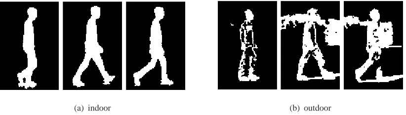
(a) indoor (b) outdoor
Fig. 1. Typical silhouettes, both (a) indoor and (b) outdoor, extracted from the HiD database. No attempt is made in this work
to ‘repair’ the damaged silhouettes typical of outdoor data.
c) Supplemental Data: The database contains supplemental images of walkers carrying
bags, rucksacks, wearing clothing such as long skirts or trenchcoats which obscure the legs,
etc. Some of these have been used to test the Bayesian framework. Although collected under
laboratory conditions, these represent difficult data, which stretch the methods developed in a
different way from the outdoor data.
B. Silhouette Extraction and Normalization
For the sequences filmed indoors, high-quality silhouettes were obtained using a chroma-key
technique. Silhouettes for the outdoor images were produced by background subtraction [18].
Figure 1 shows typical examples. To explore fully the potential of the Bayesian framework with
challenging data, no attempt is made to ‘repair’ the extracted silhouettes (contra [18]). Subsequent
processing is greatly simplified if we are able to track walkers in the scene, so allowing silhouettes
to be normalized (i.e., centered in each image). Although normalization could be simply and
straightforwardly done for the indoor data, the noise inherent in the outdoor data dictates the
use of a relatively more sophisticated approach.
For this purpose, we use an evidence-based tracking algorithm described by Lappas, Carter and
Damper [19], who extended the dynamic Hough transform to detect arbitrary shapes undergoing
arbitrary affine motion. The algorithm processes the whole image sequence globally and the
optimal object trajectory is found by maximizing its associated energy. No initialization is
required. Lappas et al. used temporal dynamic programming to achieve the optimization. The
template used for the Hough transform is the very rough contour of the upper body (head and
(a)
(b)
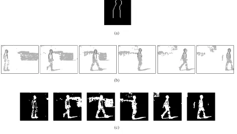
[image:6.595.72.543.126.393.2](c)
Fig. 2. Example of normalization of an outdoor image sequence: (a) shows the average template somewhat enlarged relative to
the other sequences; (b) shows a typical silhouette sequence with the best-fit position of this template superimposed; (c) shows
the final (120×120) pixel bounding box obtained.
was generated and the optimal trajectory found for each. The overall best trajectory tells us the
locations of the walker in the sequence, and the size of the optimal template is used to normalize
the silhouettes.
Figure 2 illustrates the normalization for an outdoor sequence. Fig. 2(a) shows the average
template; the sequence depicted in Fig. 2(b) shows the position found by the tracking algorithm
with the optimal template superimposed. (Note that the polarity of the silhouette has been inverted
and silhouette pixels substituted by gray to show the superimposed template more clearly.) As
seen, the walker is well located even in the presence of a passing bus. Finally, Fig. 2(c) shows
the bounding box obtained by recentering the walker. Because walkers in the indoor images are
large (in terms of number of pixels) relative to the outdoor images, they were reduced to fit in a
(70×70) bounding box. The outdoor images were simply cropped to(120×120) pixels. Images
can be smaller in the former case as (70×70) images were found adequate for bootstrapping
IV. A BAYESIAN FRAMEWORK FOR GAITEXTRACTION
Satisfying the complex requirements of extracting human gait from real-world images
de-mands decomposition into sub-problems, with the solutions to each integrated into a consistent
framework (Bayesian in this work). Our first sub-task is to define the strong prior knowledge
of shape and movement of humans via an articulated model. This is described in Section IV-A.
The variation in pose during a gait cycle is quite large. This makes fitting an articulated model
difficult as there is a large region of parameter space corresponding to feasible walkers. To
ease this difficulty, we divide the walking cycle into six sections and use an HMM to label the
images automatically depending on which part (decided empirically—see below) of the walking
cycle they come from. We build into the HMM prior knowledge of the coordinated movement
of the body parts. Section IV-B describes the automatic labeling process. In Section IV-C, we
describe the posterior probability of the model parameters given the images. This is maximized
to extract information about the gait in terms of those parameters that best fit each image. The
technical issues that arise in maximizing the posterior are discussed in Section IV-D. Finally
in Section IV-E, we detail how the priors for the model parameters are learned using Bayesian
updating. To obtain the data for this, we re-use modules developed in the rest of the framework.
A. Articulated Model
A cornerstone of our approach is the exploitation of strong prior knowledge of human walkers
and walking. The most basic level at which this knowledge is introduced is the articulated walker
model. In our view, it is important to match the complexity of the model to the quality of the
data available to us. There is no point in including and defining aspects to the model which
cannot be realistically estimated. Because we are viewing walkers from the side, we can build a
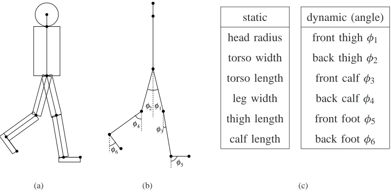
very simple 2D articulated model. Figure 3 shows the model used and lists the parameters that
control it. The basic model has 12 parameters which divide into two groups: those determining
the sizes of the body parts which remain constant for all images in the sequence; and the angles
between the body parts, which vary from frame to frame. We refer to these as static and dynamic
variables respectively.
Clearly, the model is only a crude approximation to a real walker. No account is taken of
perspective, parts of the body such as the neck, arms and hands are missing, foot lengths and
(a)
φ
φ
φ
φ
3 2 1
φ
4
6
5
φ
(b)
static dynamic (angle)
head radius front thigh φ1
torso width back thigh φ2
torso length front calf φ3
leg width back calf φ4
thigh length front foot φ5
calf length back foot φ6
[image:8.595.104.506.132.330.2](c)
Fig. 3. The basic articulated model of a walker: (a) shows the body parts; (b) defines the various joint angles; and (c) lists the
model’s static and dynamic parameters. The arms are omitted in an attempt to match the complexity of the model appropriately
to the available data. The foot length and width are fixed at 7.5 pixels and 3 pixels in the(70×70) pixel images and twice these values in the(120×120)pixel images.
right sides of the body. We rather distinguish between the front and back legs alone. Thus, our
definition of a gait cycle is half the length of the one defined in [20]. These simplifications
reduce computational complexity and are consistent with our stated philosophy of matching
model complexity to the available data. For example, there is unlikely to be sufficient information
in the outdoor images to be able to fit details such as the arms. (This has been confirmed in
preliminary work in which arms were included in the articulated model, but results were no
better than those reported later in this paper.) Furthermore, we avoid possible ambiguities in
fitting the model arising from having to determine which leg is which.
Gait information is extracted by finding the best set of model parameters to fit any given
silhouette. In the Bayesian framework, this means determining the likelihood of the image given
the model. To achieve this, we generate from the model a silhouette of the appropriate size. This
‘model silhouette’ is then matched against the observed data silhouette—see next subsection.
In the following, we denote the set of parameters of the articulated model as θ and the model
B. Locating Phase in the Gait Cycle
Our prior knowledge of walking tells us that the dynamic parameters of the articulated model
(i.e., joint angles) are a strong function of the phase within the gait cycle. The Bayesian
framework exploits this information by finding which part of the gait cycle an image comes
from. To automate this, we use a hidden Markov model (HMM). Of course, given that they
provide a natural framework for processing sequential stochastic data, HMMs have been very
popular in previous work on human gait (e.g., [21], [22], [23], [13]). In this work, we use the
Viterbi algorithm for state decoding.
Because the walking cycle is a rather simple case of cyclical motion, we took the approach
of defining a hand-crafted HMM whose parameters are chosen to reflect this prior knowledge
rather than being automatically learned from data. This prior information has been extracted
from hand-labeled data: 3 randomly chosen sequences for each of 7 walkers. The definition of
the HMM went through some iterations of improvement; its final form along with its associated
parameters are shown in Figure 4.
Originally, the walking cycle was divided into K =5 sections, each having 4 tied states, to
give a 20 state HMM. We used tied states rather than single states with self-transitions to model
the state occupancy better. The intention was that each section was occupied for approximately
the same time. Four states per section were chosen because this is a reasonable upper limit
on the number of frames per section. Skip transitions will therefore model cycles of less than
20 frames. Initial probabilities were chosen so that each state was equally likely (π =0.05).
Skip transition probabilities were chosen to reflect the distribution of state occupancy estimated
from the data of a few walkers. The largest skips (transitions p3 and q4) are included to model
possible missing frames, although these did not occur in the training data. Subsequently, it was
realized that for one particular section of the cycle, the variation in walker pose was very large
as a consequence of rapid limb movement in this phase. This occurred at the bottom of the leg
swing, where the dynamic movement is high. To remedy this, we split this section into two to
give K =6 sections with the split pair represented by 3 HMM states. The transition probabilities
were adjusted to cater for this, as listed in Fig. 4(b).
The probability of an image belonging to (i.e., being emitted by) a particular state is
START 1 1 p 1 p2 p 3
k=1
1 1 1 1 2 1 p 1 p 2 p 3
k=2
2 1 2 1 3 2 q 1 q 2 q 3 q 4
k=3
3 2 3 2 3 2 4 2 q1 q 2 q 3 q 4
k=4
4 2 4 2 4 2 5 2 q 1 q 2 q 3 q 4
k=5
5 2 5 2 5 2 6 2 q 1 q 2 q 3 q 4
k=6
6 2 6 2 6 2 (a) probabilities values
π1 0.033
π2 0.050
p1 0.475
p2 0.475
p3 0.050
q1 0.050
q2 0.530
q3 0.370
q4 0.050
[image:10.595.88.529.119.432.2](b)
Fig. 4. Hand-crafted hidden Markov model used to locate images within the gait cycle: (a) shows the architecture of the HMM
with sections labeled by an image of the corresponding prototype; (b) lists the values of transition probabilities.
the corresponding section of the walk. The prototypes embody the average articulated-model
parameters extracted from that section of the walk for each of the hand-labeled sequences.
The parameters for the prototype are denoted by {θk}K
k=1. Starting from some initial values,
the average parameters were iteratively refined by the bootstrapping method described below
(Section IV-E). To measure the distance between the images and the prototypes we use the
chamfer distance, which has been popular in object detection and tracking [24], [25], [16]. We
denote the chamfer distance between edge images x and y byρ(x, y). In this work, the chamfer
distance is computed efficiently using the chamfer distance transform. The real (silhouette)
images and the prototype images are converted to edge images using the Sobel edge detector.
The real edge images then serve as reference; they are chamfer distance transformed. We use a
(3×3) mask with a (3,4)/3 distance measure to approximate a Euclidean distance using integer
model prototype is thus ρ(x,I(θk)).
Modelling the probability of a template match is non-trivial and many methods have been
suggested. The most recent of these uses the pdf projection theorem [26], [27], [28], which
takes into account the differing discriminative abilities of the templates. This method is easily
adapted to compute the probability of an image x being emitted from state k as:
p(x|k)=g(x)
pρ(x,I(θk)) k
P
j p
ρ(x,I(θk)) jp(j)
where we model the probability of a chamfer distance ρ(x,I(θk)) being equal to r given that
x comes from the j th section of the walk by a gamma distribution:
p(r|j)= b
a
ra−1e−br Ŵ(a) .
The function g(x) is the same for all states k so does not need to be determined. Thus, to use
the pdf projection theorem we need to know the parameters a and b for each of the gamma
distributions describing the spread of chamfer distance matches between the images in section j
of the walk and the prototype for section k—giving a total of K2gamma distributions. (As we will
see in the next subsection, gamma distributions do an excellent job of modeling chamfer distance
data in this application.) These parameters will be different for the high-quality indoor data and
the noisy outdoor data. We therefore need to perform an initial calibration for each database used.
Given a set of labeled images, we can perform this calibration by first calculating the chamfer
distances between the images in each section of the walk and each of the prototypes and then
finding the parameters of the gamma distributions that maximize the likelihood of the chamfer
distance values. For the indoor data, we used the same training data as used to compute the
average prototype parameters; for the outdoor later, we hand-labeled a similar number of images.
C. Posterior Probability for Model Parameters
Having labeled each image according to its section in the walking cycle, we are in a position
to find the parameters of the articulated model which best fit each of the images. The static
parameters describing sizes of the body parts and the dynamic parameters describing the angles
of the limbs are treated differently. The static parameters are assumed to remain constant over
(a)
4 5 5 5 6 6 1 1 2 2 3 3 4 4 4 5
(b)
3 3 4 4 4 5 5 6 6 1 2 2 3 3 3 4
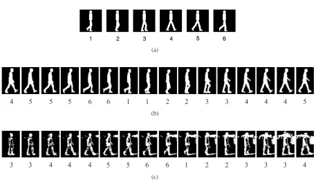
[image:12.595.80.540.109.372.2](c)
Fig. 5. Labeling the phase of the gait cycle using the HMM: (a) shows the K =6 mean models used as prototypes. Typical
labelings produced by the HMM are shown for (b) an indoor sequence and (c) an outdoor sequence.
of images. The dynamic parameters are optimized on a frame-by-frame basis. In both cases,
we maximize a posterior probability for the parameters. For the dynamic parameters, this is
the posterior given a particular image, while for the static parameters, it is the posterior given a
sequence of images. The posterior for the sequence is assumed to be the product of the posteriors
for each of the single images.
The posterior probability of the parametersθ, given an image from section k and a modelMk,
can be written as:
p(θ|x,Mk)∝ p(x|θ,Mk)p(θ|Mk)
where p(x|θ,Mk)is the likelihood of the image given the parameters and p(θ|Mk)is the prior
for the parameters. The constant of proportionality is independent of the model so does not
influence the maximum a posteriori parameters. We cannot use the pdf projection theorem for
calculating the likelihood, p(x|θ) of an image, x, given a set of model parameters, θ, because
we now have a continuum of models. Instead we follow the conventional (maximum entropy)
p(x|θ)∝e−bρ(x,I(θ))
where b is a Lagrange multiplier to be determined empirically. We make the additional assumption
that the number of images with chamfer distance ρ(x,I(θ)) equal to r grows as a
polyno-mial ra−1. That is, the distribution of chamfer distances is given by:
pρ(x,I(θ)) =r
θ
=
Z
p(x|θ) δρ(x,I(θ))−rdx ∝ra−1e−br
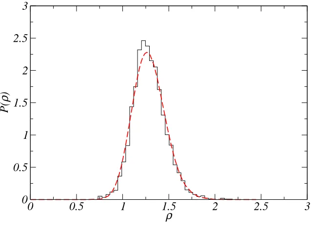
i.e., a gamma distribution. Empirically, this distribution fits the data well as shown in Figure 6,
in which the theoretical distribution is compared to a histogram of values obtained from selected
calibration data (3606 chamfer distances), chosen on the basis of good visual fit. The parameters
a and b can be found by fitting empirical data using maximum likelihood. This way to determine
the exponent b is identical to that of Toyama and Blake [16], although we give a slightly different
(and we believe more direct) motivation.
We assume a Gaussian prior for the parameters:
p(θ|Mk)∝exp−1
2(θ−θk) TC−1
k (θ −θk)
whereθk and Ck are the averages and covariances for the parameters in section k of the walk. The
average parameters are the same as those of our prototypes described in the previous subsection.
The covariance matrix is learned using Bayesian updating described in Section IV-E. In the
next subsection, we discuss the practical details of finding the parameters which maximize
the posterior probability.
D. Optimizing Parameters
The posterior probability is a highly non-linear function of the parameters θ which may
have many local maxima. To find the best-fit parameters, we use a standard multi-dimensional
continuous optimization algorithm (Powell’s method) to maximize the log-posterior. At each
iteration, we compute the likelihood between the images and a ‘silhouette model’. Pre-computing
the chamfer distance transform for all the images speeds up this computation considerably. The
chamfer distance transform is also used by the HMM in computing the likelihood of the image
0 0.5 1 1.5 2 2.5 3
ρ
0 0.5 1 1.5 2 2.5
P(
ρ
[image:14.595.147.468.121.355.2])
Fig. 6. Distribution of empirical chamfer distance values for 3606 data points selected as calibration data and fitted gamma
distribution. As can be seen, the fit is excellent.
the time taken to perform the optimization, depends on the initial values of the parameters. We
discuss our strategy for choosing these initial parameter below. Since the criteria for optimizing
the static and dynamic parameters differ, we separated the two tasks.
We start by finding the best-fit static parameters over the sequence. To achieve this, we find the
best static parameters where the dynamic parameters are chosen to be those of the appropriate
prototypeθk. The log-likelihood of the sequence of images can be computed efficiently by
sum-ming the chamfer distance transforms for the K sets of images with the same label. Calculating
the posterior for the sequence then involves K matchings of the summed, transformed images
versus the model.
The dynamic parameters are extracted on an image-by-image basis. We optimize the dynamic
parameters twice, from two different starting positions. The first initialization takes the dynamic
parameters for the corresponding prototype model. The second uses a linear prediction of the
parameters from the best parameter values found in the previous time steps. That is, denoting the
optimal parameters found in frame t by θ(t), then our initial parameter estimates in frame t+1
˜
θ(t+1)=θ(t)+(θ(t)−θ(t −1))
We choose the fit that gives the highest posterior probability after optimization.
In principle, we can refine our estimates for the static and dynamic parameters iteratively.
However, in practice, we found that after a single iteration our estimates for the model parameters
were adequate and the improvements obtained by further iterations were insignificant.
E. Bayesian Updating of Priors
Part of the prior information built into our framework is the statistics of the parameters of the
prototype model, in terms of their means {θk}K
k=1 and covariances{Ck} K
k=1. These statistics were
acquired from fitting high-quality images. To initiate the process, we used the same data as for
finding the HMM prototypes (see Section IV-B). The images were manually labeled to determine
which section of the gait cycle they came from. The framework described above was used to find
a best-fit model for the images in these sequences but using likelihoods rather than posteriors.
In addition, some hard constraints were imposed to prevent an implausible fit between an image
and model. For instance, we limited the radius of the head to be between 3 and 5 pixels. The
results were checked visually to ensure that the fitting had not failed catastrophically. The means
and covariances were calculated from the extracted models. Having obtained a reasonable first
estimate for the means and covariances, we were able to fit other high-quality sequences which
were then used to refine our prior via Bayesian updating.
V. RESULTS OFMODELFITTING
We have tested our method on various sequences in the Southampton HiD database [17],
not only the indoor, outdoor and supplemental data as outlined in Section III-A but also some
artificially modified data. The modifications tested are addition of synthetic ‘salt and pepper’
noise and addition of occluding bars. We believe it is very important to derive quantitative figures
of merit for our model-fitting results. In the case of high-quality images (i.e., indoor data), it is
sufficient to use the chamfer distance for this purpose, since the extracted silhouettes are of a
high fidelity. For outdoor data, however, the chamfer distance is unsuitable as a sole measure
close-to-correct fit. We have, therefore, established (approximate) ground truth by hand labeling
body points in a selection of images. Of course, the hand labels are not used in any way during
the extraction; they are ‘unseen’. This approximate ground truth is then used to calculate an
average pixel error per body point.
A. Indoor Data
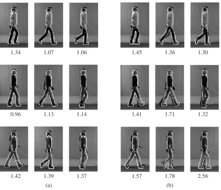
Figure 7(a) illustrates three typical extracted model sequences superimposed on the
corre-sponding high-quality indoor data. To enable the reader to judge the significance of the chamfer
distance as an error measure, their respective values are shown below each image. As can be
seen, most errors are attributable to the simplifications implicit in the model; for example, the
walker on the bottom row has a pony-tail and long tee-shirt which are not well modelled by the
rectangle-plus-circle representation of the torso and head. Nonetheless, it is clear that for the
most part, the model fitting is very good with an average error of about 1 pixel. (Recall that
edges are detected in the ‘model silhouette’ before chamfer distance computation, so that the
average quoted here is that computed across this number of edge points.)
B. Sequences with Added Synthetic Noise
To demonstrate the robustness of the system performance, salt and pepper noise was added
to 10 normalized high-quality data sequences, each of length 20 images, from different walkers.
A percentage p of pixels was randomly chosen; half of these were set to 1 and the remainder
were set to 0, irrespective of their original values. Figure 8 shows an example frame with different
levels of noise added. We then fitted models to these noisy data sequences.
Results for 50% noise are shown in Fig. 7(b) for the same (noise-free) images as in Fig. 7(a),
allowing easy comparison of the two cases and giving further insight into the interpretation of
the chamfer distance values. As expected, there is an overall increase in error which is easily
seen to result largely from poorer fitting of the dynamic parameters.
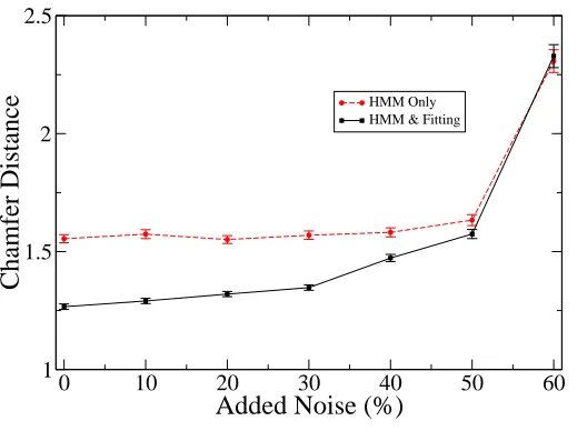
The means and corresponding error bars of the chamfer distance between the walker model and
the original (noise-free) images are shown in Figure 9 in two forms, as a function of percentage
of added noise. First, we show the best fit model obtained by optimizing dynamic and static
parameters as described in Section IV-D. These results are shown by a full line. Second, to
(a) (b)
1.34 1.07 1.06
0.96 1.13 1.14
1.42 1.39 1.37
1.45 1.36 1.30
1.41 1.71 1.32
[image:17.595.79.534.119.511.2]1.57 1.78 2.56
Fig. 7. Examples of extracted models overlaid on their original images. The models shown in (a) were found on noise-free
data whereas those in (b) were found after 50% salt and pepper noise—not shown here—had been added to the silhouettes. The
numbers below each image are the calculated chamfer distances between the fitted models and the noise-free silhouettes.
show results using only the six mean (prototype) model walkers as in Fig. 5(a). As can be seen,
the HMM is almost completely unperturbed up to 50% noise and fails catastrophically thereafter.
(Although not shown on the figure, 100% added noise gives an average error of just below
2.5 pixels. This apparently low value can be understood from the fact that normalization was
done before adding the synthetic noise, so that the average static model is automatically placed at
approximately the right place.) As expected, the gain from the additional parameter optimization
(a) 0% (b) 10% (c) 20% (d) 30% (e) 40% (f) 50% (g) 60%
Fig. 8. Examples of normalized silhouettes with added salt and pepper noise.
0 10 20 30 40 50 60
Added Noise (%)
1 1.5 2 2.5
Chamfer Distance
HMM Only HMM & Fitting
Fig. 9. Means of the chamfer distances between the models extracted from the sequences with added salt and pepper noise,
and the original clean data. The error bars shows estimated errors in the means. KEY: ‘HMM Only’ means we use only the
six mean (prototype) model walkers as in Fig. 5(a); ‘HMM & Fitting’ means we fit model walkers by optimizing dynamic and
static parameters as described in Section IV-D.
C. Sequences with Artificial Occlusion
We also tested the system on the indoor data with artificial occlusion, for the same sequences
as in the previous subsection. This is a good exemplar of difficult, structured ‘noise’ as opposed
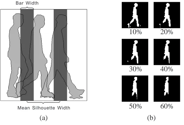
to the previously-used random salt and pepper noise. The method of occlusion is illustrated in
Figure 10(a). The walker is assumed to walk behind regularly-spaced vertical bars. The mean
width of the silhouettes in a sequence was calculated and the mid-lines of neighboring bars
arranged at intervals of this distance. The width of the bars is expressed as a proportion of this
mean width. Figure 10(b) shows an example silhouette occluded by bars with different widths.
Chamfer distances were computed between the extracted models and the clean original images
[image:18.595.155.528.146.436.2] [image:18.595.179.443.245.439.2]Mean Silhouette Width Bar Width
(a) (b)
10% 20%
30% 40%
50% 60%
Fig. 10. Artificially-occluded data: (a) illustrates how vertical bars are added to images; (b) shows a sample silhouette occluded
by bars with different widths.
of these means versus the occlusion measure. As before, results are shown using only the six
prototype walkers (dotted line) as well using fully optimized walker models (full line) in order
to make explicit the contribution of the HMM fitting procedure. It can be seen that the structured
‘noise’ presents a harder problem than random salt and pepper noise, with the system failing
almost completely at around 50% occlusion.
D. Outdoor Sequences
The real test of our approach is how well it performs on image sequences with realistic amounts
of noise, exemplified by the outdoor data. Fig. 12(a) illustrates the complexity of the problem
by showing the raw silhouettes used as inputs to the algorithm. These are clearly contaminated
with extraneous detail such as a passing bus and another walker at some distance. Although the
silhouettes could be ‘repaired’ (e.g., [18]), the techniques for doing so are ad hoc and we wished
to avoid using them because our method is intended to cope with challenging data. Fig. 12(b)
shows the models extracted from the data. To show the fidelity of the fit, Fig. 12(c) illustrates
the original images with outlines of these models superimposed. As can be seen, an accurate
fit of the model to the walker is obtained. There are some systematic errors; for example, the
[image:19.595.164.464.121.326.2]0 10 20 30 40 50 60
Occlusion (%)
1 1.5 2
Chamfer Distance
[image:20.595.178.435.122.308.2]HMM Only HMM & Fitting
Fig. 11. Means of the chamfer distances between the models extracted from the sequences which have been occluded and the
original clean data. The error bars shows estimated errors in the means. KEY: as in Fig. 9.
test illustrates the robustness of our algorithm.
These results, although typical, are illustrative only. Ideally, we wish to quantify performance
on as large a set of data as possible. The real problem in so doing is to know what counts as
correct. To approximate a ‘gold standard’, we manually marked the positions of five fiducial
points, namely the hip, front/back knee and front/back ankle, in the original data. Although
the manual labeling can never be perfect, we feel this is a reasonable, practical compromise.
The labeling was done for 10 sequences of 5 walkers from the database, each of which had
50 frames. The gait-extraction algorithm was then applied to these same sequences. We calculated
the distances from the hip, front/back knee and front/back ankle positions obtained from the
extracted models to the fiducial points in the corresponding images.
In Figure 13(a), we illustrate an example frame that has been marked manually and the
corresponding points on the model fitted to the walker in that frame are shown in Figure 13(b).
Table I shows the means and standard deviations (SD) of the distances computed for each of the
five points plus the overall mean and SD. Note that the overall mean and SD for the example
sequence shown in Figure 12 were 2.49 and 1.35 pixels respectively; this justifies our earlier
description of this sequence as ‘typical’.
We are unaware of any other system in the literature which is able to cope with this level
(a)
(b)
[image:21.595.81.538.143.436.2](c)
Fig. 12. Typical model fitting results: (a) cropped sample silhouettes; (b) extracted models, and (c) extracted models
superimposed on the raw images.
◦
A
A
′
◦
B
B
′
◦
C
C
′
◦
D
D
′
◦
[image:21.595.137.479.534.687.2]E
E
′
Fig. 13. Joint positions on walker: (a) shows an example frame from one of the video sequence where the joints were marked
MEANS AND STANDARD DEVIATIONS(SD)OF THE DISTANCES BETWEEN THE FIVE JOINTS MARKED MANUALLY ON THE OUTDOOR DATA AND THOSE OBTAINED BY FITTING THE MODEL.
(pixel) Hip Front Knee Front Ankle Back Knee Back Ankle Overall
Mean 2.94 2.27 2.43 2.19 2.62 2.49
Horizontal Mean 1.12 0.89 1.60 1.19 1.29 1.22
Vertical Mean 2.51 1.92 1.48 1.64 2.04 1.92
SD 1.57 1.40 1.50 1.30 1.53 1.49
Horizontal SD 0.81 0.70 1.43 0.91 1.00 1.03
Vertical SD 1.69 1.47 1.15 1.25 1.55 1.48
silhouettes seen in Fig. 12(a). The reason that the results are as good as they are is because
we have a consistent way of exploiting the constraints of the problem by treating them as prior
knowledge within the Bayesian framework. We accept that these constraints (i.e., uninterrupted
walk orthogonal to camera direction) do simplify the problem considerably, but this kind of data
is very typical of that used in current studies. Such data are available to us in a large database
which was expensive and time-consuming to collect, and is starting to become widely-used in
gait studies.
E. Extending the Walker Model
A severe problem with gait extraction arises when the body and limbs are obscured by, for
example, an overcoat or carried briefcase. Because our approach combines a powerful statistical
approach with a simple articulated model of a walker, it offers a straightforward way to cope
with this situation by extending the walker model. We illustrate this with three examples in
which the model is generalized by the addition of a rucksack, or a long skirt, or a trench coat.
A rucksack was represented by a half ellipse, a long skirt by filling the gaps between the legs,
and a trapezoid was added to stand for a trench coat. A maximum of two more static parameters
was needed to cater for each of the three cases.
These additions were tested on the supplemental data from the Southampton HiD database.
Tests used 4 sequences of 20 frames each from one walker for each condition (added rucksack,
(a)
(b)
[image:23.595.194.425.116.535.2](c)
Fig. 14. Fitting results: (a) carrying a rucksack, (b) wearing a long skirt, and (c) wearing a trench coat.
sequences, using average pixel joint error (Table II). As expected, for walkers wearing a long
skirt or a trench coat, the errors at the knees are larger than at other points. In spite of this,
the overall results (as judged visually) remain good. We believe the level of disruption of body
shape which occurs in these sequences would defeat most current approaches to gait extraction.
Clearly, if we were to attempt to exploit the extensibility of the framework in a real application,
it would be necessary to devise some means of performing automatically the necessary model
selection between regular, rucksack, long skirt or trenchcoat models on a particular data sequence.
MEANS AND STANDARD DEVIATIONS(SD)OF THE DISTANCES BETWEEN THE FIVE POINTS MARKED MANUALLY ON THE SEQUENCES WITH RUCKSACK,LONG SKIRT OR TRENCH COAT AND THOSE OBTAINED BY FITTING THE EXTENDED MODEL.
(pixel) Hip Front Knee Front Ankle Back Knee Back Ankle Overall
Rucksack Mean 2.24 3.53 3.79 2.47 2.71 2.95
SD 1.57 1.80 1.39 1.58 1.40 1.66
Long Mean 3.17 6.26 3.72 6.33 4.68 4.83
Skirt SD 2.19 2.70 2.48 2.64 2.41 2.80
Trench Mean 2.01 6.19 3.63 5.23 3.01 4.02
Coat SD 1.04 1.63 2.24 1.71 3.13 2.55
focus of the current paper. Accordingly, it will not be considered further here.
VI. APPLICATION TOPERSON IDENTIFICATION BY GAIT
The methods developed in this paper have obvious application to person recognition by
gait, a problem domain in which there has been significant interest in recent years [29], [30].
Furthermore, since the identity of all the walkers in the Southampton HiD database is known, we
do not confront the problem of absence of a ‘gold standard’ as was the case in the previous
model-fitting work. Performance on gait recognition therefore offers a very direct way to test the efficacy
of our algorithms, especially as there exists a well-established baseline algorithm due to Sarkar
et al. [30] for this task that can be used for comparison. This algorithm estimates silhouettes
by background subtraction and performs recognition by temporal correlation of silhouettes. For
the purposes of this paper, we use the baseline algorithm as described in [30] except that we
use the normalization procedure outlined in Section III-B earlier. Whereas the normalization in
the baseline algorithm is semi-automatic, ours is fully automatic. Results were obtained using
both the indoor and outdoor data as described in Section III-A. We did not use the HumanID
gait challenge data [30] because these feature walkers moving in a circular pattern whereas our
work has thus far been based on an assumption of fronto-parallel movement (i.e., “sideways
on”) relative to the camera. We restrict our attention to identification.
Using the Bayesian framework developed above, we find a best-fit model for each frame of
recognition; the dynamic parameters are assumed to vary periodically across frames and can be
compactly described by the coefficients of a Fourier series. For the purposes of gait recognition,
of the six dynamic parameters depicted in Fig. 3 we use only the first four, φ1 to φ4, i.e., front
thigh angle, back thigh angle, front calf angle, and back calf angle. The feet angles are omitted
because, for the outdoor data, the pixels around the feet are very noisy. Very often, the feet
are missing or connected to spurious silhouette pixels caused by shadows. For these reasons,
initial feet angles are not much different to the optimised ones, and their inclusion did not affect
results.
A. Fitting Fourier Series
We use Fourier series having a limited number of harmonics to approximate the variation of
dynamic parameters. The function F(t; f0, τ,C)returns the value of the complex Fourier series
at time t , that is:
F(t; f0, τ,C)= K
X
k=−K
ckexp 2πj f0(t +τ )
c−k =ck
where f0 is the fundamental frequency, C = {ck}k=−KK is the set of complex Fourier series
coefficients, K is the highest rank of the harmonics, and τ is a temporal adjustment to account
for the starting phase in the gait cycle.
To estimate these parameters, we find the best fit between the joint-angle trajectories extracted
from the model, φi(t), 1≤t ≤T , and the four Fourier series symbolized by F(t; f0, τ,Ci),
1≤i ≤4. We have found it sufficient to use K =3. This is done by minimizing:
E(f0, τ,C1, . . . ,C4)=
4
X
i=1 T
X
t=1
φi(t)−F(t; f0, τ,Ci)
2
with the imaginary part of c1 equal to zero for the back thigh angle. This ensures that all
trajectories align. This standard non-linear least square problem can be solved by the
Levenberg-Marquardt algorithm. Figure 15 shows the results of fitting the Fourier series to dynamic
parameters from a typical sequence.
B. Identification Results
Having fitted the Fourier series, we can use the amplitude and phase of its complex coefficients
0 5 10 15 20 25 0.2 0.25 0.3 0.35 0.4 Frame Number
Fitted Fourier Series Front Thigh Angles
(a) Front thigh angle
0 5 10 15 20 25
−0.4 −0.3 −0.2 −0.1 0 0.1 Frame Number
Fitted Fourier Series Back Thigh Angles
(b) Back thigh angle
0 5 10 15 20 25
−1 −0.8 −0.6 −0.4 −0.2 0 0.2 0.4 0.6 Frame Number
Fitted Fourier Series Front Calf Angles
(c) Front calf angle
0 5 10 15 20 25
−1 −0.8 −0.6 −0.4 −0.2 0 0.2 Frame Number
Fitted Fourier Series Back Calf Angles
[image:26.595.100.512.123.505.2](d) Back calf angle
Fig. 15. Results of fitting Fourier series to the four joint-angle trajectories extracted from a typical sequence.
walkers. However, we have obtained better performance by reweighting the features (i.e.,
com-ponents of the signature) according to their F statistics, following Lee [31]. The fundamental
frequency f0 was found to have the biggest F -statistic. Among the static parameters, only τ4
(leg width) was found to be strongly discriminative.
Identification results were obtained for our Bayesian approach and for the baseline system
on both the indoor and outdoor data. In all, 50 subjects in the gait database were selected and,
for each subject, 10 indoor and 10 outdoor sequences were taken. Both approaches were tested
using leave-one-out cross-validation with a nearest-neighbour, Euclidean distance classifier.
charac-1 2 3 4 5 6 7 8 9 10 11 12 13 14 15 0.6
0.65 0.7 0.75 0.8 0.85 0.9 0.95 1
Rank
Identification Rate
[image:27.595.165.446.125.346.2]Baseline Algorithm Our Algorithm
Fig. 16. Cumulative match characteristics for the identification of walkers from indoor data for the baseline algorithm and the
new Bayesian approach. All estimated error bars are less than 3%, and are omitted for clarity.
teristics (CMC) as described (for face recognition) in [32]. Thus, a value of N on the abscissa
(labeled ‘rank’) means that the correct walker is included within the n top-ranking candidates. The
performance of the baseline algorithm is superior in this case. It achieves 79%, 97% and 100%
identification rate at ranks 1, 5 and 10, respectively, whereas the corresponding recognition rates
for our algorithm are 61%, 92% and 99%. We interpret these results in the light that a simple
identification algorithm can do rather well on the relatively ‘easy’ indoor data; there is no
advantage to using anything more complicated. Further, we believe our algorithm is adversely
affected by the rather short sequences achievable when filming indoors, which makes fitting of the
dynamic parameters (having a strong dependence on f0) problematic. By contrast, the baseline
algorithm performs well on this high quality database because it can exploit discriminative
information about the shape of the head and upper torso.
For the much harder outdoor data, the F -statistics of most of the features are smaller than for
the indoor data, as expected. Among the static parameters, the leg width again has the largest
F -statistic. Figure 17 shows the identification results for outdoor data. The performance fell in
comparison with the indoor data. Here there is a reversal of the relative merits of the baseline
1 2 3 4 5 6 7 8 9 10 11 12 13 14 15 16 17 18 19 20 0.3
0.4 0.5 0.6 0.7 0.8 0.9
Rank
Identification Rate
[image:28.595.168.442.124.343.2]Baseline Algorithm Our Algorithm
Fig. 17. Cumulative match characteristics for the identification of walkers from outdoor data for the baseline algorithm and
the new Bayesian approach. All estimated error bars are less than 3%, and are omitted for clarity.
value of the rank.
Figure 18 shows a comparison of the rank 1 performance of the baseline algorithm and the
new Bayesian method across the indoor/outdoor conditions. The baseline method is known to
perform quite well across a range of gait recognition scenarios (see Fig. 8 of [30] where it
is noticeable that it is comparable to the best other approaches for the harder tasks). For the
relatively ‘easy’ indoor data, it outperforms our method, as we have seen. However, as stated in
Section V-D, the real test of our approach is how well it performs on the difficult (and much
more realistic) outdoor data. Here, we see that our new algorithm does significantly better than
the baseline algorithm.
To evaluate the contribution of the various kinds of features to the overall performance of the
Bayesian algorithm, we have rerun the tests using static parameters alone, dynamic parameters
alone and f0alone. Results for the outdoor data are shown in Figure 19; those for the indoor data
were very similar in shape. As expected, the dynamic features provided most of the biometric
information, but even the fundamental frequency plays some part in discriminating walkers.
Indoor Outdoor 0
20 40 60 80 100
Identification Rate (%)
[image:29.595.171.443.154.340.2]Baseline Algorithm Our Algorithm
Fig. 18. Comparison of the rank 1 performance of the baseline algorithm and the new Bayesian method across the indoor/outdoor
conditions. Error bars are plus/minus one standard deviation estimated on the assumption of binomial distribution of errors.
1 2 3 4 5 6 7 8 9 10 11 12 13 14 15 16 17 18 19 20 21 22 23 24 25 0
0.1 0.2 0.3 0.4 0.5 0.6 0.7 0.8 0.9 1
Rank
Recognition Rate
All Features Static Parameters Dynamic Parameters Fundamental Frequency
Fig. 19. Contribution to the identification performance of the Bayesian approach made by subsets of extracted gait features
[image:29.595.169.442.464.689.2]VII. CONCLUSIONS
We have described a consistent Bayesian framework for addressing the important and
well-studied problem of human gait extraction from video sequences, and established the utility of the
method by applying it to biometric identification of humans. The framework developed allows
us to integrate strong prior knowledge with data-driven learning and thereby to produce results
comparable with the best reported in the literature, handling noise and occlusion especially
well. Results of model-fitting have been quantified on a large database which is becoming
increasingly available, opening the way for other researchers to compare their results objectively
with ours. The individual component parts of the overall system are themselves quite simple;
the power comes from the Bayesian framework. We regard a degree of simplicity as a virtue,
since the component parts of the system can be easily extended and modified, as illustrated in
the extensions of the articulated model to cope with rucksacks, long skirts, etc.
Within the computer-vision community, there has been a (very understandable) tendency to
focus on novel—and therefore usually complex—component parts of such a system. These have
often been built into a Bayesian framework, yet the vital contribution made by the framework has
not always been fully recognized. Advances in this field are, we believe, at least as likely to come
from the adoption of a consistent, extensible and principled framework using well-established
component techniques as from a search for novel, sophisticated algorithms. In our opinion, a
key contribution of this paper is to illustrate the advantages of deploying an appropriate mix of
strong prior knowledge and simple but powerful learning methodologies in just the way that the
Bayesian framework allows.
ACKNOWLEDGEMENT
We are indebted to M. S. Nixon and J. N. Carter, who kindly made the Southampton HiD
database available for this work.
REFERENCES
[1] C. C´edras and M. Shah, “Motion-based recognition: A survey,” Image and Vision Computing, vol. 13, no. 2, pp. 129–155,
1995.
[2] T. B. Moeslund and E. Granum, “A survey of computer vision-based human motion capture,” Computer Vision and Image
[3] L. Wang, W. Hu, and T. Tan, “Recent developments in human motion analysis,” Pattern Recognition, vol. 36, no. 3, pp.
585–601, 2003.
[4] J. O’Rourke and N. I. Badler, “Model based image analysis of human motion using constraint propagation,” IEEE
Transactions on Pattern Analysis and Machine Intelligence, vol. 2, no. 6, pp. 522–536, 1980.
[5] D. C. Hogg, “Model-based vision: A program to see a walking person,” Image and Vision Computing, vol. 1, no. 1, pp.
5–20, 1983.
[6] A. M. Baumberg and D. C. Hogg, “An efficient method for contour tracking using active shape models,” in Proceedings
of IEEE Workshop on Motion of Non-Rigid and Articulated Objects, Austin, TX, 1994, pp. 194–199.
[7] K. Rohr, “Towards model-based recognition of human movement in image sequences,” CVGIP, Image Understanding,
vol. 59, no. 1, pp. 94–115, 1994.
[8] S. X. Ju, M. J. Black, and Y. Yacoob, “Cardbord people: a parameterized model of articulated motion,” in Proceedings of
2nd International Conference on Automatic Face and Gesture Recognition, Killington, VT, 1996, pp. 38–44.
[9] J. K. Aggarwal and Q. Cai, “Human motion analysis: A review,” Computer Vision and Image Understanding, vol. 73,
no. 3, pp. 428–440, 1999.
[10] H. Ning, L. Wang, W. Hu, and T. Tan, “Articulated model based people tracking using motion models,” in Proceedings of
IEEE International Conference on Multimodal Interfaces, Pittsburgh, PA, 2002, pp. 383–388.
[11] A. Elgammal, V. Shet, Y. Yacoob, and L. S. Davis, “Learning dynamics for exemplar-based gesture recognition,” in
Proceedings of IEEE International Conference on Computer Vision and Pattern Recognition, vol. 1, Madison, WI, 2003,
pp. 571–578.
[12] A. Elgammal, “Nonlinear generative models for dynamic shape and dynamic appearance,” in Proceedings of 2nd
International Workshop on Generative-Model Based Vision, Washington, DC, 2004, pagination unknown.
[13] X. Lan and D. P. Huttenlocher, “A unified spatio-temporal articulated model for tracking,” in Proceedings of IEEE
International Conference on Computer Vision and Pattern Recognition, vol. 1, Washington, DC, 2004, pp. 722–729.
[14] L. Sigal, S. Bhatia, S. Roth, M. J. Black, and M. Isard, “Tracking loose-limbed people,” in Proceedings of IEEE
International Conference on Computer Vision and Pattern Recognition, vol. 1, Washington, DC, 2004, pp. 421–428.
[15] J. Zhang, R. Collins, and Y. Liu, “Representation and matching of articulated shapes,” in Proceedings of the 2004 IEEE
Conference on Computer Vision and Pattern Recognition (CVPR’04), vol. II, Washington, DC, 2004, pp. 342–349.
[16] K. Toyama and A. Blake, “Probabilistic tracking with exemplars in a metric space,” International Journal of Computer
Vision, vol. 48, no. 1, pp. 9–19, 2002.
[17] J. Shutler, M. Grant, M. S. Nixon, and J. N. Carter, “On a large sequence-based human gait database,” in Proceedings of
4th International Conference on Recent Advances in Soft Computing, Nottingham, UK, 2002, pp. 66–72.
[18] M. G. Grant, J. D. Shutler, M. S. Nixon, and J. N. Carter, “Analysis of a human extraction system for deploying gait
biometrics,” in IEEE Southwest Symposium on Image Analysis and Interpretation, Lake Tahoe, NV, 2004, pp. 46–50.
[19] P. Lappas, J. N. Carter, and R. I. Damper, “Robust evidence-based object tracking,” Pattern Recognition Letters, vol. 23,
no. 1–2, pp. 253–260, 2002.
[20] M. P. Murray, “Gait as a total pattern of movement,” American Journal of Physical Medicine, vol. 46, no. 1, pp. 290–329,
1967.
[21] D. Meyer, J. P¨osl, and H. Niemann, “Gait classification with HMMs for trajectories of body parts extracted by mixture
[22] L. Lee, G. Dalley, and K. Tieu, “Learning pedestrian models for silhouette refinement,” in Proceedings of IEEE International
Conference on Computer Vision, Nice, France, 2003, pp. 663–670.
[23] A. Sundaresan, A. Roy Chowdhury, and R. Chellappa, “A hidden Markov model based framework for recognition of
humans from gait sequences,” in Proceedings of IEEE International Conference on Image Processing, vol. 2, Barcelona,
Spain, 2003, pp. 85–88.
[24] G. Borgefors, “Hierarchical chamfer matching: A parametric edge matching algorithm,” IEEE Transactions on Pattern
Analysis and Machine Intelligence, vol. 10, no. 6, pp. 849–865, 1988.
[25] D. Gavrila, “Pedestrian detection for a moving vehicle,” in Proceedings of European Conference on Computer Vision,
Dublin, Ireland, 2000, pp. 37–49.
[26] P. M. Baggenstoss, “The PDF projection theorem and the class-specific method,” IEEE Transactions on Signal Processing,
vol. 51, no. 3, pp. 672–685, 2003.
[27] T. Minka, “Exemplar-based likelihoods using the PDF projection theorem,” Microsoft Research Ltd., Cambridge, UK,
Tech. Rep., March, 2004.
[28] A. Thayananthan, R. Navaratnam, P. H. S. Torr, and R. Cipolla, “Likelihood models for template matching using the PDF
projection theorem,” in Proceedings of British Machine Vision Conference (BMVC 2004), Kingston, UK, 2004, pagination
unknown.
[29] M. S. Nixon, J. N. Carter, D. Cunado, P. S. Huang, and S. V. Stevenage, “Automatic gait recognition,” in Biometrics –
Personal Identification in Networked Society, A. K. Jain, R. Bolle, and S. Pankanti, Eds. Dordrecht, The Netherlands:
Kluwer Academic Publishers, 1999, pp. 231–249.
[30] S. Sarkar, P. J. Phillips, Z. Liu, I. R. Vega, P. Grother, and K. W. Bowyer, “The HumanID gait challenge problem: Data
sets, performance and analysis,” IEEE Transactions on Pattern Analysis and Machine Intelligence, vol. 27, no. 2, pp.
162–177, 2005.
[31] L. Lee, “Gait analysis for classification,” Artificial Intelligence Laboratory, MIT, Cambridge, MA, Tech. Rep. 2003-014,
2003.
[32] P. J. Phillips, H. Moon, S. A. Rizvi, and P. J. Rauss, “The FERET evaluation methodology for face-recognition algorithms,”
IEEE Transactions on Pattern Analysis and Machine Intelligence, vol. 22, no. 10, pp. 1090–1104, 2000.
Adam Pr ¨ugel-Bennett obtain a BSc in Physics at the University of Southampton and a PhD in Theoretical Physics at the University of Edinburgh. He worked in research jobs in Oxford, Paris, Manchester, Copenhagen and Dresden before finally returning to Southampton as a Senior Lecturer in the School of Electronics and Computer Science. His main areas of research are evolutionary algorithms, machine learning and computer vision.
Bob Damper (M’87–SM’89) obtained his MSc in Biophysics in 1973 and PhD in Electrical Engi-neering in 1979, both from the University of London. He also holds the Diploma of Imperial College, London, in Electrical Engineering. He was appointed Lecturer in Electronics at the University of Southampton in 1980, Senior Lecturer in 1989, Reader in 1998 and Professor in 2003. His research interests include signal and pattern processing, speech science and technology, computational linguistics, data engineering, and theoretical aspects of artificial intelligence. Prof. Damper has published approximately 280 articles and authored the undergraduate text Introduction to Discrete-Time Signals and
Systems. He is a past Chair of the Signal Processing Chapter of the UK and Republic of Ireland Section of the IEEE,