Multiobjective optimization using surrogates

MULTIOBJECTIVE OPTIMIZATION USING SURROGATES

Ivan Voutchkov*, A. J. Keane

CEDG, School of Engineering Sciences University of Southampton, Highfield, Southampton SO17 1BJ,

*e-mail:

[email protected]

ABSTRACT

Until recently, optimization was regarded as a discipline of rather theoretical interest, with limited real-life applicability due to the computational or experimental expense involved. Multiobjective optimization was considered as a utopia even in academic studies due to the multiplication of this expense. This paper discusses the idea of using surrogate models for multiobjective optimization. With recent advances in grid and parallel computing more companies are buying inexpensive computing clusters that work in parallel. This allows, for example, efficient fusion of surrogates and finite element models into a multiobjective optimization cycle. The research presented here demonstrates this idea using several response surface methods on a pre-selected set of test functions. It shows that a careful choice of response surface methods is important when carrying out surrogate assisted multiobjective search.

1. INTRODUCTION

In the world of real engineering design, often there are multiple targets which manufacturers are trying to achieve. For instance in the aerospace industry, a general problem is to minimize weight, cost and fuel consumption while keeping performance and safety at a maximum. Each of these targets might be easy to achieve individually. An airplane made of balsa wood would be very light and will have low fuel consumption, however it will not be structurally strong enough to perform at high speeds or carry useful payload. Also such an airplane would not be safe, i.e., robust to various weather and operational conditions. On the other hand, a solid body and a very powerful engine will make the aircraft structurally sound and able to fly at high speeds, but its cost and fuel consumption will increase enormously. So engineers are continuously solving the problem of making trade-offs and producing designs that will satisfy as many requirements as possible, while industry, commercial and ecological standards are at the same time getting ever tighter.

Multiobjective optimization (MO) is a tool that aids engineers in choosing the best design in a world where many targets need to be satisfied. Unlike conventional optimization, MO will not produce a single solution, but rather a set of solutions, most commonly referred to as Pareto front (PF). By definition it will contain only

non-dominated solutions. It is up to the engineer to select a final design by examining this front.

2.SURROGATE MODELS FOR OPTIMIZATION

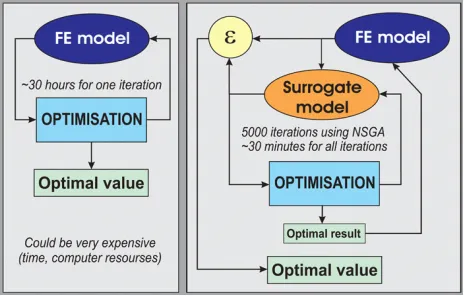
The aim of MO is to produce a well spread out set of optimal designs, with as few function evaluations as possible. There are number of methods published and widely used to do this – MOGA, SPEA, PAES, VEGA, NSGA2, etc. Some are better than others - generally the most popular in the literature are NSGA2 (Deb) and SPEA2 (Zitzler), because they are found to achieve good results for most problems [2-6]. The first is based on genetic algorithms and the second on an evolutionary algorithm, both of which are known to need many function evaluations. In real engineering problems the cost of evaluating a design is probably the biggest obstacle that prevents extensive optimization procedures. In the multiobjective world, the cost is multiplied, because there are multiple expensive results to obtain. Evaluating directly a finite element model can take several days, which makes it impossible to try hundreds or thousands of designs.

accurate replica. This makes optimization not only useful, but usable and affordable.

The key idea that makes surrogate models efficient is that they should become more accurate in the region of interest as the search progresses, rather than being equally accurate over the entire design space, as an FE representation will tend to be. This is achieved by adding to the surrogate knowledge base only at points of interest. The procedure is referred to as surrogate update.

Various publications address the idea of surrogates models and multiobjective optimisation [10 – 19]. As one would expect, no approximation method is universal. Factors such as function modality, number of variables, number of objectives, constraints, computation time, etc. all have to be taken into account when choosing an approximation method. The work presented here aims to demonstrate this diversity and hints at some possible strategies to make the best use of surrogates.

3.MULTIOBJECTIVE OPTIMIZATION USING SURROGATES

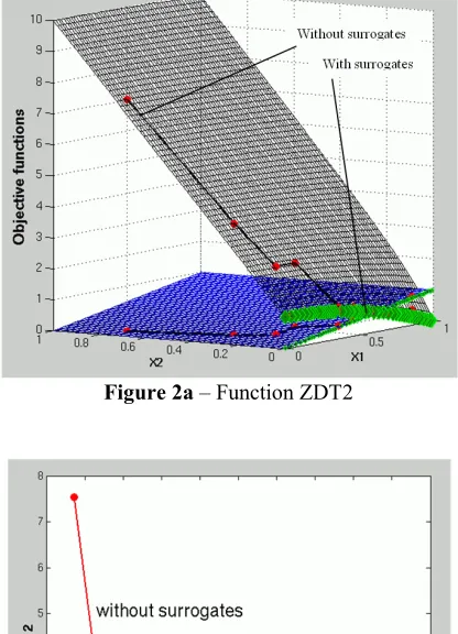
To illustrate the idea, the zdt2 function will be used. It is a good function to demonstrate the effectiveness of surrogate models, as it is fairly simple for response surface (surrogate) modelling. Figure 2 represents the function and the optimisation procedure. It is a striking comparison, demonstrating the idea. The problem has two objective functions and two design variables. The pareto front obtained using surrogates with 40 function evaluations is far superior to the one without surrogates and the same number of function evaluations. On the other hand 2500 evaluations without surrogates were required to obtain similar quality of pareto front as in the case with surrogates and 40 evaluations. The difference is even more significant if more variables are added – see Table 1.

Here we have chosen a set of objective functions with simple shapes to demonstrate the effectiveness of using surrogates. Both functions would be readily approximated using most of the methods. It is not uncommon to have relationships of similar simplcity even in reality, although external noise factors would make them look rougher.

Relationships of higher order of multimodality would be more of a challenge for most methods, as will be demonstrated later.

Figure 2a – Function ZDT2

Figure 2b – ZDT2 – Pareto front achieved in 40 evaluations: Diamonds – pareto front with surrogates;

Circles – solution without surrogates

Table 1 – Full function evaluations for Problem 1 – Figure 2

Number of variables 2 5 10 Number of function

evaluations without

surrogates 2500 5000 10000

Number of function evaluations with

4.LOCAL AND GLOBAL PARETO FRONTS

Similar to the single objective optimization, in the multiobjective world, it is also possible to have local and global optimal solutions. This concept is demonstrated using the F5 test function. Figure 3 illustrates the function and the optimization procedure, again with and without surrogates.

Figure 3 – Problem 2: Achieved in 100 evaluations: Diamonds – pareto front with surrogates; Circles –

solution without surrogates

Due to the sharp nature of the global solution it cannot be guaranteed that with a small number of GA evaluations, the correct solution will be found. Further more, since the surrogate is based only on sampled data, if this data does not contain any points in the global optimum area, then the surrogate will never know about its existence.

Therefore any optimization based only on such surrogates will lead us to the local solution. Therefore conventional optimization approaches based on surrogate models rely on constant updating of the surrogate. A widely accepted technique in the single objective optimization is to update the surrogate with its optimal solution. In multiobjective terms this will translate to updating the surrogate with one or more points belonging to its pareto front. If the surrogate pareto front is local and not global, so the next update will also be around the local pareto front.

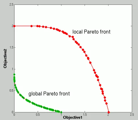
Continuing with this procedure the surrogate model will become more and more accurate in the area of the local optimal solution, but will never know about the existence of the global solution. So it turns out that the success of multiobjective optimization based on surrogates, using updates at previously found optimums strongly depends on the initial data used to train the first surrogate before any updates were added. If this data happens to contain points around the global pareto front, then the algorithm will be able to quickly converge and find a nice global pareto front, as on Figure 3. However the odds are that the local pareto fronts are smoother and easier to find shapes and in most cases this is where the procedure will converge. Figure 4 illustrates the difference of the local and global pareto fronts for the test function considered. Various approaches to escape from the local solution exist. Some are more efficient than others: a comparison will be provided in a further publication.

Figure 4 – Some problems may have deceptive features and local solutions.

5. RESPONSE SURFACE METHODS, OPTIMIZATION PROCEDURE AND TEST FUNCTIONS

efficient RS model for cases where it is expensive to obtain large amounts of data. A significant number of publications discuss the kriging procedure in detail. An important role for the success of the method is the tuning of its hyper parameters. It should be mentioned that researchers who have chosen correctly the training procedure, report positive results when using kriging, while publications who use basic training procedures reject this method. Nevertheless, the method is becoming increasingly popular in the world of optimization as often it provides a surrogate with reasonable or good accuracy.

This method was used to build surrogates for the above two test cases, therefore it is useful to briefly outline its pros and cons:

Pros:

• can always predict with no error at sample points

• the error in close proximity to sample points is minimal

• requires small number of sample points in comparison to other response surface methods

• reasonably good behaviour with high dimensional problems.

Cons:

for large number of data points and variables training of the hyper-parameters and prediction may become computationally very expensive

Researchers should make a conscious decision when choosing Kriging for their RSMs. Such a decision should take into account the cost of a direct function evaluation including constraints if any, available computational power, and dimensionality of the problem. Sometimes it might be possible to use kriging for one of the objectives while the other is evaluated directly, or a different RSM is used to minimize the cost. In other cases it might be more feasible not to use RSMs at all, as this might be the more expensive solution. Discussion of other methods will be given in the following sections of this paper.

A number of other response surface methods exist. There is a selection of several methods which will be considered in this paper that do not require initial pre-training procedure [1]. The following list details all 12 methods which will be considered in the present paper:

SRSM: Shepard response surface model LRBF: linear Radial Basis Function TPRBF: thin plate Radial Basis Function CSRBF: cubic splines Radial Basis Function

CSRBF1: cubic splines Radial Basis Function with regression via reduced bases

MPRM: mean polynomial regression model PRM11: first order polynomial regression model

PRM12: first order polynomial regression model plus squares

PRM13: first order polynomial regression model plus products (cross-terms)

PRM21: second order polynomial regression model PRM22: second order polynomial regression model

plus cubes

KRIG: Stochastic process modelling - Kriging

Other RS methods exist, such as neural networks and fuzzy logic, however we believe that the above set is representative extract of methods that can illustrate the idea of multiobjective optimization using surrogates.

As this paper aims to overview the usage of several methods, the optimization procedure and its settings will be kept the same while the RS method used to build the surrogate will change. The chosen multiobjective algorithm is NSGA2. Other multiobjective optimizers might show slightly different behaviour. The procedure is as follows:

1. Carry out 20 LPt [8] spaced initial direct function evaluations.

2. Train hyper-parameters (only for

kriging)

3. Run NSGA2 on the RSM, population

size 50 for 50 generations.

4. Select 20 evenly spaced points from the pareto front in objective space as well as in parameter space, by using the corresponding Euclidian distances as a measure.

5. Evaluate these 20 points

6. Add results to the existing data

pool of direct function evaluations

7. If data pool is larger than 150

points, choose the best 150 points in terms of closeness to the last pareto front. This measure is once again the average euclidian distance between a point being considered and all points on the last Pareto front. 8. Rank the data pool and extract the

real pareto front

9. Repeat 20 times from point 2.

There are several possible stopping criteria 1. Fixed number of update iterations

2. Stop when all update points are non-dominated 3. Stop if the percentage of new update points that

belong to the Pareto front falls below a pre-defined value

4. Stop if the percentage of old points on the current Pareto front rises above a pre-defined value

own. The best Pareto front could be defined as the one being as close as possible to the origin of the objective function space, while having the best diversity, i.e. spread on all objectives and the points are evenly distributed. Metrics for assessing the quality of the Pareto front will be discussed also in a further publication.

Four test function with various complexity have been chosen to carry out the overview of the RS methods for the purpose of multiobjective optimization. These functions are well known from the literature:

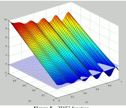
Figure 5 – ZDT3 function

ZDT2: (Figure 2). convex shaped pareto front. The two objectives are very smooth with no sharp features. Two objectives, n variables (in the present study n= 2 ), no constraints. x(i) = 0 .. 1, i= 1, 2 [3 – page 357]

F5: (Figure 3). High shape complexity – has a smooth and a sharp feature. The combination of both makes it easier for the optimization procedure to converge to the smooth feature, which represents a local Pareto front. The global Pareto front lies around the sharp feature which is harder to reach. Two objectives, x(i) = 0 .. 1, i = 1, 2; no constraints. [3 – page 350]

ZDT3: (Figure 5). Clustered and discontinued Pareto front. Shape complexity is moderate. Two objectives, n variables (in present study n= 2 ), no constraints. x (i) = 0 .. 1, i = 1, 2 [3 – page 357]

ZDT3-10: (Figure 5). Same as above, however using n = 10

ZDT2

( )

( )

(

)

(

)

( )

( ) (

)

f g f g f h x n x g x x f n i i , 1 , , 1 9 1 1 2 2 1 1 2 1 1 = = + = = = F5

( )

(

)

(

)

( )

(

) ( ) (

)

f x x f g otherwise g f if g f g f h x if x x if x x g , , 4 1 75 . 3 25 . 0 , 0 , , 1 , 1 4 . 0 , 02 . 0 2 . 0 exp 2 4 4 . 0 0 , 02 . 0 2 . 0 exp 3 4 1 2 2 1 2 1 1 1 1 1 1 2 2 2 2 2 2 2 = = + = = = ZDT3

( )

( )

(

)

(

)

( )

( ) (

)

f f g f g f g f h x n x g x x f n i i , 10 sin 1 , , 1 9 1 1 2 1 1 1 1 2 1 1 = = + = = =

6.RESULTS

A study has been carried out using all of the above response surface methods. The performance quality of each method is measured by the distance of the members of the Pareto front it produced to the true solution. The distance of the resultant Pareto front is monitored after each update. The closeness measure is defined as the average distance from a each point on the achieved pareto front and the closest point on the ‘real Pareto front’. The latter has been obtained using 20000 direct function evaluations using NSGA2 (Population size of 100 and 200 generations)

immediately. This is due to a weakness that conventional surrogate models exhibit. To explain this we would like to stress the fact that surrogate models need updating in order to improve their accuracy only where it is needed – around the area of optimal Pareto solutions. For functions that have no deceptive Pareto front features this is a very good scheme. However it fails in multimodal cases. The sole reason is that the points for the next update are taken from the previously found Pareto front. In this case – it is easier to find the deceptive Pareto front and this is where the surrogate is being updated. Due to lack of sufficient information about the rest of the objective surfaces, most of the methods see the deceptive Pareto front as the ‘best’ solution and take no action to explore. One can see that kriging, manages to utilise any information even away from the optimum and manages to construct a more representative response surface. Therefore – it is less influenced by this weakness and manages to advance towards the real pareto optimal set of solutions.

Figure 6 – Closeness to the true pareto front for F5

Figure 7 – Pareto fronts for F5

Figure 8, 8a and 9 represent the performance of all methods, when applied to ZDT3 function. In this case with 2 variables.

Figure 8 – Closeness to the true pareto front for ZDT3

Figure 8a – Zoomed version of Figure 8.

Figure 10 – Closeness to the true pareto front for ZDT3 – 10 variables

Figure 11 – Pareto fronts for ZDT3 – 10 variables It is seen that all methods rapidly achieve the optimal solution as the function has no deceptive features and sine curves are no challenge for most methods. Shepard RSM and Linear Radial basis functions converge with some delay in relation to the rest, but it is interesting to observe on Figure 9a that both of them get closest to the real pareto front. The same function can be run with 10 variables, which changes the picture of performance. Figures 10 and 11 demonstrate that kriging is the best performing method even with 10 variables.

Figures 12, 12a and 13 illustrate the performance of all methods with the very simple function ZDT2. As expected all methods but one, reach the true pareto front immediately after the first update. Shepard Response surface methods struggles down the way but never get as close as the other methods. It is interesting to mention that on a zoomed in scales, linear radial basis functions reach closest to the target, although are a bit slow at the beginning.

Figure 12 – Closeness to the true pareto front for ZDT2

Figure 12a – Zoomed version of figure 12

7.CONCLUSIONS,CURRENT AND FUTURE WORK

The ultimate aim of using surrogates for optimization is to reduce the number of function evaluations. A real life multiobjective optimization may have several objectives and several constraints, all of which need to be evaluated at each iteration. If some prior knowledge about the shape of each objective and constraint is gathered, then it is possible to devise a mixture of RSM methods which will give the best combination of accuracy and computational expense. Some of the constraints or objectives might be so simple and quick to compute, that it might be more feasible to evaluate them directly, while others use surrogates.

The results obtained here show that the performance of all methods depends on the features of the objective functions being optimized. Kriging appears to perform well in most situations, however it is much more computationally expensive than the rest. It is obvious that a careful consideration of RSM could lead to a situation where all objectives in a multiobjective problems are modelled using different methods, in order to maintain high quality and reduce optimization costs.

In general, the Cubic spline RBF is a good method that combines low cost and relatively to other methods quick convergence. For harder functions, Kriging appears to be the method to choose. Simple wave like functions can be approximated using Shepard functions, as it is the quickest RSM in the considered set. Amongst the polynomial methods, PRSM12 would be a good choice for wavy and simple feature functions.

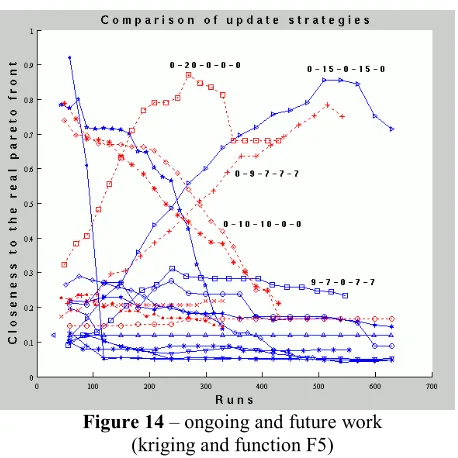
Figure 14 – ongoing and future work (kriging and function F5)

An important weakness in the conventional surrogate update strategy has been discussed, causing most of the

methods to converge around local features and thus missing the global solutions. Currently work is being carried out to investigate methods that overcome this difficulty. Figure 14 demonstrates a snapshot of a research aiming to produce the best update strategy. This work will be published soon as a journal publication. For the purpose of the current paper, it is suffice to say that the figure represents various update strategies, using kriging and function F5. It is interesting to compare some of them to Figure 6. It is obvious that a good strategy can significantly reduce the number of required function evaluations.

8.ACKNOWLEDGEMENTS

This work was funded by Rolls – Royce Plc, whose support is gratefully acknowledged.

9.REFERENCES

1. Keane, A. J, OPTIONS manual,

http://www.soton.ac.uk/~ajk/options.ps

2. S. Obayashi, S. Jeong, K. Chiba, “Multi-Objective Design Exploration for Aerodynamic Configurations”, AIAA-2005-4666

3. Deb, K., Multi-objective optimization using evolutionary algorithms, John Wiley & Sons, Ltd., New York, 2003.

4. Zitzler et al, Comparison of multiobjective evolutionary algorithms: Empirical results. Evolutionary computational journal 8(2), 125-148. 2000

5. Knowles, J. and Corne, D. (1999) The Pareto archived evolution strategy: A new baseline algorithm for multiobjective optimisation. Proceedings of the 1999 Congress on EvolutionaryComputation, Piscatway: New Jersey: IEEE Service Center, 98–105.

6. Fonseca, C. M. and Fleming, P. J. (1998) Multiobjective optimization and multiple constraint handling with evolutionary algorithms–Part II: Application example. IEEE Transactions on Systems, Man, and Cybernetics: Part A: Systems and Humans. 38–47.

7. D. R. Jones, M. Schonlau and W. J. Welch, Efficient global optimization of expensive black-box functions, Journal of Global Optimization, Vol. 13, pp. 455-492, 1998

8. I.M.Sobol', V.I. Turchaninov, Yu.L. Levitan, B.V. Shukhman: "Quasi-Random Sequence Generators" Keldysh Institute of Applied Mathematics, Russian Acamdey of Sciences, Moscow (1992)

10. Takayasu Kumano, et al, (Jannuary 2006), Multidisciplinary Design Optimization of Wing Shape for a Small Jet Aircraft Using Kriging Model, 44th AIAA Aerospace Sciences Meeting and Exhibit, pp 1 – 13

11. Nain, P. K. S. and Deb, K (March, 2005). A multi-objective optimization procedure with successive approximate models. KanGAL Report No. 2005002. 12. Andy Keane, Prasanth Nair, June 2005,

Computational Approaches for Aerospace Design: The Pursuit of Excellence, ISBN: 0-470-85540-1 13. S. Leary, A. Bhaskar, and A. J. Keane, "A derivative

based surrogate model for approximating and optimizing the output of an expensive computer simulation," J. Global Optimization 30 pp. 39-58 (2004)

14. S. Leary, A. Bhaskar, and A. J. Keane, "A Constraint Mapping Approach to the Structural Optimization of an Expensive Model using Surrogates", Optimization and Engineering 2 pp. 385-398 (2001)

15. M. Emmerich and B. Naujoks. Metamodel-assisted multiobjective optimization strategies and their application in airfoil design. In I. Parmee, editor, Proc of. Fifth Int'l. Conf. on Adaptive Design and Manufacture (ACDM), Bristol, UK, April 2004, pages 249{260, Berlin, 2004. Springer.

16. Giotis A.P., Giannakoglou K.C. “Single- and Multi-Objective Airfoil Design Using Genetic Algorithms and Artificial Intelligence”, EUROGEN 99, Evolutionary Algorithms in Engineering and Computer Science, May 1999

17. Knowles, J and Hughes, E. J. (2005) Multiobjective optimization on a budget of 250 evaluations. Evolutionary Multi-Criterion Optimization (EMO 2005), LNCS 3410, pp. 176-190, Springer-Verlag. 18. Chafekar, D. et al. Multi-objective GA optimization

using reduced models. IEEE SMCC 35(2):261-265, 2005