Eigenanalysis and continuum modelling of pre-twisted
repetitive beam-like structures
N.G. Stephen
*, Y. Zhang
School of Engineering Sciences, Mechanical Engineering, University of Southampton, Highfield, Southampton SO17 1BJ, UK
Received 19 May 2005 Available online 11 July 2005
Abstract
A repetitive pin-jointed, pre-twisted structure is analysed using a state variable transfer matrix technique. Within a global coordinate system the transfer matrix is periodic, but introduction of a local coordinate system rotating with nodal cross-sections results in an autonomous transfer matrix for this Floquet system. Eigenanalysis reveals four real unity eigenvalues, indicating tension–torsion coupling, and equivalent continuum properties such as Poissons ratio, cross-sectional area, torsion constant and the tension–torsion coupling coefficient are determined. A variety of real and complex near diagonal Jordan decompositions are possible for the multiple (eight) complex unity eigenvalues and these are discussed in some detail. Analysis of the associated principal vectors shows that a bending moment pro-duces curvature in the plane of the moment, together with shear deformation in the perpendicular plane, but no bend-ing–bending coupling; the choice of a structure having an equilateral triangular cross-section is thought responsible for this unexpected behaviour, as the equivalent continuum second moments of area are equal about all cross-sectional axes. In addition, an asymmetric stiffness matrix is obtained for bending moment and shearing force coupling, and pos-sible causes are discussed.
2005 Elsevier Ltd. All rights reserved.
Keywords: Pre-twist; Repetitive; Floquet; Jordan canonical forms; Eigenproblem; Tension–torsion; Bending–shear; Continuum; Homogenisation; Properties
1. Introduction
Repetitive (or periodic) structures are analysed most efficiently when that periodicity is taken into ac-count. It is possible to determine the behaviour of the complete structure from analysis of a single repeating
0020-7683/$ - see front matter 2005 Elsevier Ltd. All rights reserved. doi:10.1016/j.ijsolstr.2005.05.023
* Corresponding author. Tel.: +44 (0) 23 80592359; fax: +44 (0) 23 80593230.
E-mail address:[email protected](N.G. Stephen).
cell, together with knowledge of the boundary conditions. Straight (prismatic) repetitive one-dimensional (beam-like) structures have previously been analysed by Stephen and Wang (1996) as an eigenproblem for a state vector transfer matrix. The state vectorssLandsRconsist of the nodal displacement and force
components on the left- and right-hand sides, respectively, of the single cell of the repetitive structure, while the transfer matrix Gis obtained through manipulation of the single cell stiffness matrix, K. Non-unity eigenvalues of Goccur as reciprocals, and describe the rate of decay of self-equilibrated end loading, as anticipated by Saint-Venants principle. Multiple unity eigenvalues pertain to the transmission modes of tension, torsion, bending moment and shear, together with the rigid body displacements and rotations. From knowledge of the eigen- and principal vectors associated with the unity eigenvalues, equivalent con-tinuum beam properties of cross-sectional area, Poissons ratio, second moment of area, torsion constant and shear coefficient were calculated. The present paper extends this approach to pin-jointed structures
Nomenclature
A cross-sectional area
d member diameter
d nodal displacement vector
E Youngs modulus
F force vector
G,G shear modulus, transfer matrix
H height of cell cross-section (H ¼pffiffiffi3L=2) i,I,I pffiffiffiffiffiffiffi1, second moment of area, identity matrix
J,J, Jm torsion constant, Jordan block and canonical form, metric
K, K stiffness matrix, coupling coefficient
L length of cell, and of cross-sectional members, left
M bending or twisting moment
n,N,Nindex of cell or section, compliance matrix
p period
Q shearing force
R radius of bending curvature, right s state vector
T tensile force
T orthogonal coordinate transformation matrix
u,v,w displacements in thex-,y- andz-directions
v eigenvector
V similarity/transformation matrix of eigen- and principal (generalised) vectors w principal vector
x,y, z global Cartesian coordinate system at the zeroth nodal location a pre-twist angle per cell
c shear angle
e direct strain
h (torsional) rotation about the x-axis j shear coefficient
k decay factor, eigenvalue m Poissons ratio
having a pre-twisted form. Each cell has a constant angle of pre-twist, taken to be an integer fraction of 2p, so that one has a spatial, rather than the more usual temporal, periodic Floquet system.
For continuum structures, pre-twist produces tension–torsion and bending–bending couplings, and has been studied widely (see the review byRosen (1991)citing over 200 references) because of the importance of the engineering applications, ranging from turbine blades and propellers, to architectural columns. It is easy to visualise that a pre-twisted beam will increase in length if a twisting moment is applied in a direction tending to decrease the pre-twist angle; equivalently, a tensile force will produce both an extension and a reduction in pre-twist angle. Bending–bending coupling is not so easy to visualise: consider a straight beam, such as a metal ruler, for which the bending stiffnessin the two principal planes are quite unequal; if subject to excessive compressive load, buckling would favour deflection in the flexible plane. Suppose, now, that this beam has a total uniform pre-twist through 90, and that a bending moment is applied at one end (left-hand, say) in the flexible planeat that end; at the right-hand end, the moment is in the stiff plane. Thus at the two ends, there would be curvature in just one plane; bending deflection would again favour the flexible plane, and be much greater at the left-hand end. The above is easy to visualise: less so, is the behaviour at locations between the two ends. If there is a coupled bending curvature perpendicular to that of the applied bending moment, then clearly its magnitude must vary from zero to zero over the 90
twist of the beam; in turn, there are two obvious possibilities: either that it depends on double the pre-twist angle in a sinusoidal form, or that it remains zero throughout. Existing theories are based on the former; however the example pre-twisted structure considered in the present paper does not exhibit such bending– bending coupling, presumably because the chosen equilateral triangular cross-section has equal equivalent continuum second moments of area about all cross-sectional axes. On the other hand, the example structure does exhibit a bending-shear coupling, which is not included in the majority of such theories.
Previous research on continuum pre-twisted structures may be classified as within the spirit ofStrength of Materials, or the more exact three-dimensionalTheory of Elasticity. The former is based largely upon the so-calledhelical fibre assumptionfirst introduced byChen (1951),1in which the longitudinal stress in the bar cross-section is not parallel to the axis, but acts in the direction of the longitudinal spiral fibres of the pre-twisted bar. The typical approach of the latter, see for exampleOkubo (1951, 1953, 1954), Goodier and Griffin (1969), Shield (1982), Krenk (1983a,b), Pucci and Risitano (1996) and Guglielmino and Saccomandi (1996), is the introduction of a local coordinate system, which rotates with the principal axes of the cross-section, into the governing differential equations for stress describing force equilibrium, or the equivalent (Navier) equations for displacements; while the equilibrium equations become more complicated, the advantage is that the traction-free boundary condition becomes independent of the axial coordinate. In the present work, the introduction of a local coordinate system rotating with the cross-section leads to a transfer matrix which is autonomous, that is, independent of location; one now has translational symmetry, allowing eigenanalysis.
The paper is laid out as follows: in Section 2, we describe the example structure; a pin-jointed framework was chosen so that predictions from the present approach could be verified by comparison with exact finite element analysis (FEA). In Section 3, the transfer matrix approach is outlined for a straight structure, the necessary modifications for a pre-twisted structure and the relationship with Floquet theory are noted. Coordinate transformations leading to the autonomous transfer matrix are developed, and its symplectic properties noted. In Section 4, eigenanalysis of the autonomous transfer matrix is performed, and the vari-ety of possible real and complex Jordan block decompositions introduced and discussed; apart from some example-specific decay eigenvalues, the analysis is applicable to any repetitive pre-twisted structure. Section 5 describes the coupling of eigen- and principal vectors according to the real Jordan block forms, from which the example-specific equivalent continuum beam properties are determined. Conclusions are drawn
1
in Section 6, and the transformation matrix leading to the real Jordan block form, and modified shear vec-tors are presented in Appendices A and B.
2. Example structure
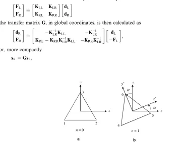
We consider a pin-jointed beam-like framework whose cross-section is in the form of an equilateral tri-angle of side lengthL= 0.3428 m. The zeroth nodal cross-section is assumed to align with a globalx y z
coordinate system (x is the axial direction), Fig. 1(a), while the adjacent n= 1 nodal cross-section, Fig. 1(b), is pre-twisted through anglearadians, here taken asa=p/8; also shown is a local coordinate system
x0y0z0which rotates with the cross-section. The axial length of the cell is also taken to be L= 0.3428 m. Individual members of the cell are of aluminium, having Youngs modulusE= 70·109N/m2and diameter
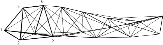
d= 6.35 mm. The longitudinal (helical) members, together with the two diagonals in each external face of the cell, have length as demanded by the relevant nodal locations, that is, the pre-twisted structure is free of any pre-load. The complete first cell of the framework,Fig. 2, is shown in bold.
3. Transfer matrix
For a straight repetitive structure, the stiffness matrixKfor a typical cell is first constructed employing the global coordinate system which is, of course, applicable to all cells; cross-sectional members are re-garded as being shared by adjacent cells, so are treated as having one-half of their actual stiffness. The stiff-ness matrix relates nodal force and displacement components as
FL
FR
¼ KLL KLR
KRL KRR
d
L
dR
ð1Þ
the transfer matrixG, in global coordinates, is then calculated as
dR
FR
¼ K
1
LRKLL KLR1
KRLKRRKLR1KLL KRRKLR1
" #
dL
FL
; ð2Þ
or, more compactly
sR ¼GsL; ð3Þ
y
z y
z
1 2
3
4
5 6
n= 0 n= 1
a b
α α
y′
[image:4.544.44.404.363.648.2]z′
where the state vectors, and the transfer matrixG, are defined accordingly. In the above, the subscripts L and R are employed to denote left- and right-hand sides of the cell, whileGis the same for all cells; the force vector withinsLrequires a minus sign, as the state vectors are defined according to the conventions of the
Theory of Elasticity, rather than FEA. The above is an adequate description for the straight structure, which possesses translational symmetry, but is inadequate for the pre-twisted structure for which, in global coordinates, the transfer matrix for each cell within a cycle is different. Instead we write for the first cell,
Fig. 2,
sð1Þ ¼Gð1Þsð0Þ; ð4Þ
and for the typicalnth cell
sðnÞ ¼GðnÞsðn1Þ; ð5Þ
where the state vector subscript has been replaced by an argument, to denote the nodal location, and the transfer matrixGrequires an index to identify the cell.
Assuming that the pre-twist anglea for each cell is constant, then the transfer matrixG(n) is periodic, with periodp= 2p/a, that is
GðnþpÞ ¼GðnÞ; ð6Þ
and for the present example p= 16. For simplicity, suppose that theNth nodal cross-section aligns with the global coordinate system; so too will the (N+p)th. Suppose that one constructs a stiffness matrix for allpcells, and then condense this to form a super-element stiffness matrixKprelating force and displace-ment components on theNth and the (N+p)th nodal locations. Note that the subscript p has been em-ployed to denote a complete cycle of p cells. From this, one could construct a transfer matrix Gp, using Eq. (2), which is known as the monodromy matrix; note that Gp¼P
p
n¼1GðnÞ. One could then perform
eigenanalysis in the usual way; that is, denoting the state vectors as sp(N) and sp(N+p), respectively, gives
spðNþpÞ ¼GpspðNÞ and spðNþpÞ ¼kpspðNÞ ð7Þ
to give the eigenproblem
ðGpkpIÞspðNÞ ¼0. ð8Þ
Denote the square matrix comprised of the eigen- and principal vectors of the above asVp(N); this trans-forms the transfer matrix to the Jordan canonical form Jp, according to
VpðNÞ 1
GpVpðNÞ ¼Jp. ð9Þ
The process described above allows one to treat the pre-twisted beam as if it were straight; however, state vectors are only defined at those cross-sections that align with the global coordinate system, and
1
2 3
6
4
[image:5.544.135.415.95.173.2]5
the information contained within the eigen- and principal vectors describes the behaviour of a complete cycle ofp cells. Such a procedure is exactly how periodic systems are often treated using Floquet theory; see, for example,Kelley and Peterson (2001). The eigenvalues kpare known as Floquet multipliers, and define the stability of a (usually dynamic) periodic system which most often is all that is required.
Instead, introduce an autonomous transfer matrix G0, which is independent of the cell index, n, by employing a local coordinate system; refer toFig. 1for the first cell, and note that the left-hand side aligns with the globalx y z coordinate system. The local right-hand side nodal coordinates transform as
x0
y0
z0
2 6 4
3 7 5¼
1 0 0
0 cosa sina 0 sina cosa
2 6 4
3 7 5
x
y
z
2 6 4
3 7 5¼T3
x
y
z
2 6 4
3 7
5; ð10Þ
where the 3·3 orthogonal transformation matrixT3is defined accordingly. On the other hand, nodal
dis-placement and force components, referring to node 4 inFig. 1(b), transform as
F04x
F04y
F04z
2 6 4
3 7 5¼
1 0 0
0 cosa sina 0 sina cosa
2 6 4
3 7 5
F4x
F4y
F4z
2 6 4
3 7 5¼TT3
F4x
F4y
F4z
2 6 4
3 7
5 ð11Þ
and
d04x
d04y
d04z
2 6 4
3 7 5¼
1 0 0
0 cosa sina 0 sina cosa
2 6 4
3 7 5
d4x
d4y
d4z
2 6 4
3 7 5¼TT3
d4x
d4y
d4z
2 6 4
3 7
5. ð12Þ
Extending this scheme to the other nodes, the state vector on the right-hand side may be written in the local coordinate system as
s0ð1Þ ¼TT18sð1Þ; ð13Þ
whereTT18 is the 18·18 transformation matrix consisting of TT3 blocks on the leading diagonal, but zero elsewhere. Now pre-multiply Eq.(4) byTT18 to give
TT18sð1Þ ¼TT18Gð1Þsð0Þ; ors0ð Þ ¼1 G0sð0Þ; ð14Þ
where
G0¼TT18Gð1Þ. ð15Þ
y
z
7
8
9
n= 2 2α
2α
y′′
[image:6.544.39.493.167.363.2]z′′
Each cell within the cycle requires a transformation matrix to relate the local coordinate system with the global, although this is not required for the eigenanalysis; the pattern is easily discerned by considering the second cell, Fig. 3, (where a double prime notation is temporarily, and somewhat unsatisfactorily, em-ployed) whose local right-hand side coordinates transform as
x00
y00
z00
2 6 4
3 7 5¼
1 0 0
0 cosa sina 0 sina cosa
2 6 4
3 7 5
x0
y0
z0
2 6 4
3 7 5¼
1 0 0
0 cosa sina 0 sina cosa
2 6 4
3 7 5
2
x
y
z
2 6 4
3 7 5¼
1 0 0
0 cos 2a sin 2a 0 sin 2a cos 2a
2 6 4
3 7 5
x
y
z
2 6 4
3 7 5
¼T3ð2Þ
x
y
z
2 6 4
3 7
5; ð16Þ
where the index 2 denotes a rotation by angle 2a, and the transformation matrix for the first cell strictly requires index 1. Suppose that the transfer matrix for this second cell had been calculated in global coor-dinates according tos(2) =G(2)s(1). In the local coordinatesfor this cell, one hass0ð2Þ ¼TT18ð2Þsð2Þ, and s0ð1Þ ¼TT18ð1Þsð1Þ, or s(1) =T18(1)s0(1), since the transformation matrix is orthogonal. Pre-multiply by
TT18ð2Þ in the above to give TT18ð2Þsð2Þ ¼TT18ð2ÞGð2Þsð1Þ or s0(2) =G0(2)s0(1) where G0ð2Þ ¼
TT18ð2ÞGð2ÞT18ð1Þ.
For the nth cell, one has in global coordinates s(n) =G(n)s(n1); in local coordinates s0ðnÞ ¼TT18ðnÞsðnÞ, s(n1) =T18(n1)s0(n1). Pre-multiply by TT18ðnÞ in the above to give
TT18ðnÞsðnÞ ¼TT18ðnÞGðnÞsðn1Þors0(n) =G0(n)s0(n1) so the transformation for the general cell is
G0ðnÞ ¼TT18ðnÞGðnÞT18ðn1Þ; ð17Þ
note that for the first cell, this reduces to Eq.(15)asT18(0) is the identity matrix.
Expressed within the local coordinates of the cell under consideration, the transfer matrix is invariant; that is
G0¼G0ð1Þ ¼ ¼G0ðnÞ ¼G0ðpÞ. ð18Þ
The transfer matrix G0 has the property of being symplectic, as doesG(1); each satisfies the relationship
GTJmG=Jm, whereJmis the metric matrixJm¼
0 I
I 0
,Iis the identity matrix of the appropriate size,
andJTm¼Jm1¼ Jm. ForG(1), this can be proven by direct substitution from Eq.(2), and noting that the
stiffness matrixKis symmetric. ForG0, start from the relationshipG(1)T
JmG(1) =Jm, and substitute from
Eq.(15)to giveG0TTT18JmT18G0¼Jm; last, partition the transformation matrix asT18¼
T9 0
0 T9
, and
ex-pand to find thatTT18JmT18is equal toJm, noting that the transpose ofT9is equal to its inverse.
4. Eigenanalysis
Since the structure, using the local coordinate system, now possesses translational symmetry, two con-secutive state vectors are related by the scalar kas
s0ðnþ1Þ ¼ks0ðnÞ; ð19Þ
which, together with the transfer matrix relation, s0(n+ 1) =G0s0(n), immediately leads to the eigenvalue problem
Although the transfer matrixG0is identical for all cells, we specifically consider the first cell, for which the left-hand cross-section aligns with the global coordinate system; this facilitates interpretation of the ei-gen- and principal vectors.
Theeigcommand within MATLAB gives the eigenvalues of the transfer matrixG0as the three reciprocal pairs
k1¼ 22.3303
k11¼ 0.0488
; k2¼ 10.0110ð1þiÞ
k21¼ 0.0499ð1iÞ
;
k2¼ 10.0110ð1iÞ
k21¼ 0.0499ð1þiÞ
" #
; ð21Þ
which describe decay of self-equilibrated loading, and four real unity eigenvalues pertaining to rigid body displacement in, and rigid body rotation about, thex-direction, together with tension and torsion. Also there are eight complex unity eigenvalues of the form 4·e±ia, in whichais the angle of pre-twist per cell, and these relate to rigid body displacements in, and rigid body rotations about, both they- andz-directions, together with bending moments and shearing forces in both planes.
As with the eigenanalysis described byStephen and Wang (1996), the eigenvectors associated with the distinct decay eigenvalues are correctly calculated by the QR algorithm employed within MATLAB, and these are designatedv1tov6. On the other hand, the eigenvectors describing rigid body displacements in
thex-direction,v7, and rotation about thex-axis,v9, are determined from the reduced row echelon form
(rref) of (G0I), and may be written as
v7¼½1 0 0 1 0 0 1 0 0 0 0 0 0 0 0 0 0 0 T
108; ð22Þ
v9¼½0 Lh=2 Hh=3 0 Lh=2 Hh=3 0 0 2Hh=3 0 0 0 0 0 0 0 0 0 T
; ð23Þ
where the angle of rotation is arbitrarily taken to beh= 5·108rad. Two principal vectorsw8andw10are
coupled tov7andv9, respectively and are found using the MATLABrrefcommand on the augmented
ma-trix, again as described byStephen and Wang (1996), followed by appropriate interpretation. Principal vec-torw8, consists of the necessary combination of tensile force and twisting moment which, when applied to
the left- and right-hand sides of the cell, produces the unit extension defined by eigenvectorv7on the right.
Principal vector w10 consists of the necessary combination of twisting moment and tensile force which,
when applied to the left- and right-hand sides of the cell, produces the rotation defined by eigenvectorv9
on the right. Two 2·2 Jordan blocks are associated with these vectors, which are
J2ð1Þ2¼J2ð2Þ2¼ 1 1
0 1
. ð24Þ
A variety of strategies are possible for determination of the eigen- and principal vectors associated with the multiple complex unity eigenvalues, 4·e±ia. For example, two chains of equations relating eigen- and principal vectors may be expressed as
G0eiaI
v11¼0 G0eiaI
v15¼0;
G0eiaI
w12¼v11 G0eiaI
w16¼v15;
G0eiaI
w13¼w12 G0eiaI
w17¼w16;
G0eiaI
w14¼w13 G0eiaI
w18¼w17.
ð25Þ
The reduced row echelon forms of the matrices (G0eia
I) and (G0eia
I), respectively, yields the two eigenvectors
v11¼½0 i 1 0 i 1 0 i 1 0 0 0 0 0 0 0 0 0 T
108; ð26Þ
which are a combination of real and imaginary rigid body displacements in the y- and z-directions. The principal vectors w12to w14andw16 tow18 can then be determined by following the chains, Eqs.(25). If
one then constructs a similarity matrix Vfrom these eigen- and principal vectors, this gives the Jordan canonical form (JCF) at its simplest
J¼V1G0V¼
k1 0 0 0 0 0 0 0 0 0
0 k2 0 0 0 0 0 0 0 0
0 0 k2 0 0 0 0 0 0 0
0 0 0 k11 0 0 0 0 0 0
0 0 0 0 k21 0 0 0 0 0
0 0 0 0 0 k21 0 0 0 0
0 0 0 0 0 0 Jð21Þ2 0 0 0
0 0 0 0 0 0 0 Jð22Þ2 0 0
0 0 0 0 0 0 0 0 Jð41Þ4 0
0 0 0 0 0 0 0 0 0 Jð42Þ4
2 6 6 6 6 6 6 6 6 6 6 6 6 6 6 6 6 6 6 6 6 6 6 6 4 3 7 7 7 7 7 7 7 7 7 7 7 7 7 7 7 7 7 7 7 7 7 7 7 5
; ð28Þ
where the two 4·4 Jordan blocks associated with the multiple complex unity eigenvalues are
Jð41Þ4¼
eia 1 0 0 0 eia 1 0 0 0 eia 1 0 0 0 eia
2 6 6 6 4 3 7 7 7 5; J
ð2Þ
44¼
eia 1 0 0
0 eia 1 0
0 0 eia 1
0 0 0 eia
2 6 6 6 4 3 7 7 7
5. ð29a;bÞ
Now, while the JCF may be in its simplest form, because of the complex eigenvalues, and complex eigen-and principal vectors, interpretation of the vectors is at its most difficult. A complex vector is not physically permissible, but when considered in conjunction with its conjugate, the (real) displacement and force com-ponents are the real and imaginary parts, in turn. Indeed, if one replaces the complex conjugate columns of the similarity matrix by their real and imaginary parts, one obtains the real JCF
J¼
k1 0 0 0 0 0 0 0 0
0 realðk2Þ imagðk2Þ 0 0 0 0 0 0
0 imagðk2Þ realðk2Þ 0 0 0 0 0 0
0 0 0 k11 0 0 0 0 0
0 0 0 0 realðk2Þ imagðk2Þ 0 0 0
0 0 0 0 imagðk2Þ realðk2Þ 0 0 0
0 0 0 0 0 0 Jð21Þ2 0 0
0 0 0 0 0 0 0 Jð22Þ2 0
0 0 0 0 0 0 0 0 J88
2 6 6 6 6 6 6 6 6 6 6 6 6 6 6 6 6 6 6 4 3 7 7 7 7 7 7 7 7 7 7 7 7 7 7 7 7 7 7 5
where
J88¼
c s 1 0 0 0 0 0
s c 0 1 0 0 0 0
0 0 c s 1 0 0 0
0 0 s c 0 1 0 0
0 0 0 0 c s 1 0
0 0 0 0 s c 0 1
0 0 0 0 0 0 c s
0 0 0 0 0 0 s c
2 6 6 6 6 6 6 6 6 6 6 6 6 6 4
3 7 7 7 7 7 7 7 7 7 7 7 7 7 5
; ð31Þ
withc¼cosa,s¼sina; note that the single complex unity eigenvalues on the leading diagonal are replaced by 2·2 real blocks. Within this formulation, the principal vectorsw13andw14describe rigid body rotations
of the left-hand side of the cell, but employ the localy0- andz0-axes of the right-hand cross-section, respec-tively. In turn, their coupled principal vectorsw15, w16,w17 andw18describe bending moment and shear
vectors applied to the left-hand side of the cell, but employ the local coordinate system of the right-hand side of the cell. For interpretation of these vectors, it is easier if they are expressed within the local coor-dinate system of the left-hand side, for which the local and global coorcoor-dinate systems coincide. This is achieved by employing a near diagonal Jordan decomposition in which the complex unity eigenvalue re-places the real unity on the super diagonal; the chains then become
ðG0eiaIÞv
11¼0; ðG0eiaIÞv15¼0;
ðG0eiaIÞw12¼eiav11; ðG0eiaIÞw16¼eiav15; ðG0eiaIÞw13¼eiaw12; ðG0eiaIÞw17¼eiaw16;
ðG0eiaIÞw
14¼eiaw13; ðG0eiaIÞw18¼eiaw17.
ð32Þ
The new complex similarity matrix V comprised of these eigen- and principal vectors transforms the transfer matrixG0 into a new JCF, which remains broadly as in Eq. (28), but with two new 4Æ4 blocks, which are
Jð41Þ4¼
eia eia 0 0 0 eia eia 0 0 0 eia eia 0 0 0 eia
2 6 6 6 4
3 7 7 7 5; J
ð2Þ
44¼
eia eia 0 0 0 eia eia 0 0 0 eia eia
0 0 0 eia
2 6 6 6 4
3 7 7 7
5. ð33Þ
Again, this leads to complex conjugate eigen- and principal vectors, and replacing these by their real and imaginary parts, allows one to construct a new real similarity matrix which transformsG0into a new real JCF, which differs from Eq.(31), in that the 8·8 block becomes
J88¼
c s c s 0 0 0 0
s c s c 0 0 0 0
0 0 c s c s 0 0
0 0 s c s c 0 0
0 0 0 0 c s c s
0 0 0 0 s c s c
0 0 0 0 0 0 c s
0 0 0 0 0 0 s c
2 6 6 6 6 6 6 6 6 6 6 6 6 6 4
3 7 7 7 7 7 7 7 7 7 7 7 7 7 5
This real similarity matrix Vand the associated JCF are given in Appendix A. The eigen- and principal vectors pertaining to the multiple complex unity eigenvalues are now expressed within the global coordinate system of the left-hand cross-section. This greatly simplifies the physical interpretation of these vectors and, in turn, determination of the equivalent continuum properties.
5. Equivalent continuum properties
5.1. Tension–torsion coupling
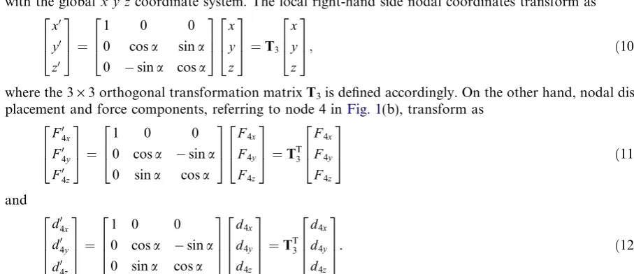
The two vectorsv7andw8are coupled according to
G0w8¼w8þv7 ð35Þ
as shown inFig. 4, where it is seen that a tensile force and a twisting moment are applied on both hand sides of the cell in order to produce unit extension in thex-direction, only. The two vectorsv9andw10are
cou-pled according to
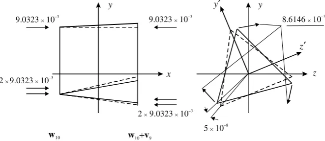
G0w10¼w10þv9 ð36Þ
as shown inFig. 5, where it is seen that a twisting moment and a compressive force are applied on both sides of the cell in order to produce rotation about the x-axis, only. Following Di Prima (1959), ten-sion–torsion coupling is expressed as
T
Mx
¼ EA Ktt
Ktt GJ
u=L
h=L
ð37Þ
whereKttis the coupling coefficient. From vectorsw8andv7, the quantitiesT,Mxandu are known (h is zero), and the equivalent cross-sectional area and coupling coefficient are calculated as A= (0.22941·
0.3428)/(70·109·1·108) = 1.1234·104m2, and Ktt=1.8578·105N m. Additionally, there is a Poissons ratio effect on the cross-section; the strain in the x-direction is ex= 1·108 /0.3428 = 2.9172·108, while the strains in the y- and z-directions are ey ¼ ð1.68830.8442Þ 109= ð0.3428pffiffiffi3=2Þ ¼ 8.5306109;ez¼ ð1.6214109Þ=0.3428¼ 8.5306109. Employingm=ey/ex=
x z
y
1.6883 10–9
×
8.4417 1010
× –
1 10× –8
7.6469 102
× –
2 7.6469 10× × –2
7.6469 102
× –
2 7.6469 102
× × –
9.1274 102
× –
1.4612 109
× – 1.4612 109
× – w8
y
[image:11.544.115.434.501.635.2]w8 v7
ez /ex, the Poissons ratio is calculated asm= 0.2924. In turn, an equivalent shear modulus is found as
G=E/(2(1 +m)) = 27.081·109N/m2, with Youngs modulusEbeing regarded as invariant.
From vectorsw10andv9, quantitiesT,Mxandhare known (uis zero), and Eq.(37)give the equivalent torsion constant and coupling coefficient as J¼ ð8.61461030.3428=pffiffiffi3Þ= ð27.0811095
108Þ ¼1.2949106m4, and K
tt=1.8578 ·105Nm, respectively; the latter is identical to that found from vectorsw8andv7, as one would expect from the reciprocal theorem.
5.2. Rigid body rotations
The two principal vectorsw13andw14are coupled to the rigid body displacement eigenvectorsv11andv12
according to the scheme
G0w13¼v11cosaþv12sinaþw13cosaþw14sina;
G0w14¼ v11sinaþv12cosaw13sinaþw14cosa.
ð38a;bÞ
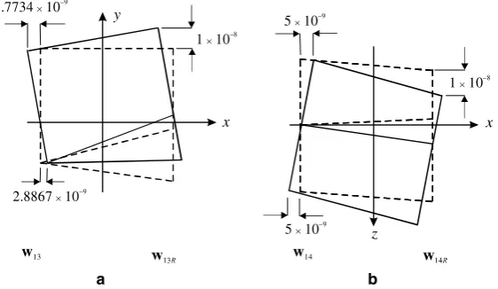
Vectorsw13and w14describe rigid body rotations of the left-hand cross-section about the z- andy-axes,
respectively, within the global coordinate system. Pre-multiplication of these vectors by the transfer matrix G0will give rigid body rotations of the right-hand side about the localz0- andy0-axes, respectively, as indi-cated by Eq.(14). However interpretation of these vectors is easier when these right-hand rotations are ex-pressed within the global coordinate system, which is achieved by pre-multiplication byG, according to
w13R¼Gw13;w14R¼Gw14 ð39Þ
whereGis the transfer matrix defined within the global coordinate system for this first cell, and the addi-tional subscriptRdenotes the right-hand side vector; these vectors are shown in Fig. 6.
5.3. Bending moments
Principal vectorsw15andw16describe the bending moments on the left-hand side of the cell in thexy
-andxz-planes, respectively, within the global coordinate system, and are coupled to the rotations according to
G0w15¼w13cosaþw14sinaþw15cosaþw16sina;
G0w16¼ w13sinaþw14cosaw15sinaþw16cosa.
ð40a;bÞ
x z
y
9.0323 10–3
×
2 9.0323 10× × –3
9.0323 103
× –
2 9.0323 103
× × –
w10
5 108
× –
8.6146 103
× –
y y′
[image:12.544.103.434.96.240.2]z′
Again, pre-multiplication byG0would give the two bending moment vectors on the right-hand side of the cell in the local x0y0- and x0z0-planes, and for interpretation of the vectors, it is preferable that these right-hand vectors be expressed within the global coordinate system, which is achieved by pre-multiplica-tion byG, to give
w15R¼Gw15; w16R¼Gw16. ð41Þ
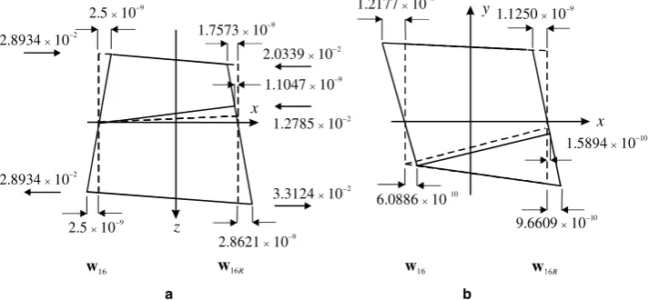
Analysis of thex-direction displacement components of the left-hand cross-section within vectorsw15and
w16, shows that both are comprised of two rotations about they- andz-axes, and can be decomposed as
d1x
d2x
d3x
2 6 4 3 7 5 w15 ¼a
d1x
d2x
d3x
2 6 4 3 7 5 w13 þb
d1x
d2x
d3x
2 6 4 3 7 5 w4 ;
d1x
d2x
d3x
2 6 4 3 7 5 w16 ¼c
d1x
d2x
d3x
2 6 4 3 7 5 w14 þd
d1x
d2x
d3x
2 6 4 3 7 5 w13
. ð42a;bÞ
Similar analysis of these components within the right-hand side vectorsw15Randw16R, shows that they
are also comprised of two rotations about they- andz-axes, and can be decomposed as
d4x
d5x
d6x
2 6 4 3 7 5 w15R ¼e
d4x
d5x
d6x
2 6 4 3 7 5 w13R þf
d4x
d5x
d6x
2 6 4 3 7 5 w14R ;
d4x
d5x
d6x
2 6 4 3 7 5 w16R ¼g
d4x
d5x
d6x
2 6 4 3 7 5 w14R þh
d4x
d5x
d6x
2 6 4 3 7 5 w13R .
ð43a;bÞ
Simple calculations from Eqs.(42) and (43)givea=0.5,b= 0.2109,c=0.5 andd=0.2109, for the left-hand side, ande= 0.5,f= 0.2109,g= 0.5 andh=0.2109 for the right; the fact that coefficientsaand
eare equal but of opposite sign indicates a curvature of the cell, while the equality of coefficientsb andf
indicates a shear deformation of the cell, as shown inFigs. 7 and 8. FromFigs. 7(a) and 8(a), the two bend-ing curvatures in thexy- andxz-planes, respectively, are
1 Ry
¼owz
ox ¼1.443410 9 H 3 L 2
¼8.5098108m1;
1 Rz
¼owy
ox ¼2.510 9 L 2 L 2
¼8.5098108m1;
ð44a;bÞ x
5.7734 10× –9
1 10× –8
w13 2.8867 10× –9
5 10× –9
5 10× –9
1 10× –8
y
z
x
a b
w14
[image:13.544.136.417.94.257.2]while consideration of Figs. 7(b) and 8(b) gives the two coupled shear angles in thexz- and xy-planes, respectively, as
cxz¼1.0546109=ðL=2Þ ¼6.1527109;
cxy ¼6.088610
10=
6.08861010=ðH=2Þ ¼6.1527109. ð45a;bÞ
The above indicates that a bending moment produces a curvature in the plane of bending, together with a shear deformation in the perpendicular plane, and is consistent with the bending theory of pre-twisted beams presented byTabarrok and Xiong (1989). It should be noted that the bending moment vectors also contain self-equilibrating nodal forces in they- andz-directions, although these are not shown inFigs. 7
and 8, which implies that the resultant nodal force is not in the axial direction. Such additional
compo-nents of force are not required from consideration of force or moment equilibrium, but rather from nodal
w16 w16
2.5 10× –9
z
x
x y
2.5 10× –9 2.8934 10× –2
2.8934 10× –2
2.0339 10× –2
1.2785 10× –2
3.3124 10× –2 1.7573 10× –9
1.1047 10× –9
2.8621 10× –9
a b
1.2177 10× –9
6.0886 10× 10
1.1250 10× –9
1.5894 10× –10
[image:14.544.101.437.98.258.2]9.6609 10× –10
Fig. 8. Principal vectorw16, for bending moment in thexz-plane: (a) and (b) show the displacement and force components in thexz -andxy-planes, respectively.
x
2.8868 10× –9
w15
y
z
x
2.6670 10× –9
1.4434 10× –9
2.2902 10× –9
3.7680 10× –10 3.3410 10× –2
2×1.6705×10–2
3.0867 10× –2
4.3609 10× –2
2.6506 10× –2
a b
1.0545 10× –9
1.0545 10× –9
4.6600 10× –10 7.4130 10× –10
[image:14.544.91.448.315.480.2]1.2073 10× –9 w15
displacement compatibility requirements of adjacent cells. In contrast to many theories of pre-twisted beams, there is no evidence of bending–bending coupling, that is, curvature in two perpendicular planes produced by the moment.
5.4. Shearing forces
Principal vectors w17 and w18 are coupled to the bending moments on the left-hand side of the cell,
according to
G0w17¼w15cosaþw16sinaþw17cosaþw18sina;
G0w18¼ w15sinaþw16cosaw17sinaþw18cosa.
ð46a;bÞ
Previous experience from the eigenanalysis of a straight repetitive structure suggests that these two vec-tors should describe shear; however analysis of the force components within vecvec-tors w17and w18gives a
resultant shear forceQy, and momentsMz,Myfor the former, and a resultant shear forceQz, and moments
My,Mzfor the latter. In fact, onlyQyandMz, andQzandMyare required to define the simplest left-hand shear vectors in thexy- andxz-planes, respectively, such that one should have a shearing force only on the right-hand side of the cell, and the unnecessary bending moments are removed according to the scheme
w17¼w17
resultantðMyÞ withinw17
resultantðMyÞ withinw16 w16;
w18¼w17
resultantðMzÞwithinw18
resultantðMzÞwithinw15 w15.
ð47a;bÞ
The two new shear vectorsw17 andw18are given in Appendix B. Again, it is preferable that the shear vectors on the right-hand side of the cell should be given within the global coordinate system, and these are determined by
w17R¼Gw17; w18R¼Gw18; ð48Þ
these describe the shear vectors in thexy- andxz-planes on both sides of the single cell, in global coordi-nates, in their simplest forms.
Again, consideration of thex-direction displacement components in the left-hand side vectorsw17 and w18 shows that they can be decomposed into rotations about they- andz-axes, as
d1x
d2x
d3x
2 6 4 3 7 5 w 17 ¼a
d1x
d2x
d3x
2 6 4 3 7 5 w13 þb
d1x
d2x
d3x
2 6 4 3 7 5 w14 ;
d1x
d2x
d3x
2 6 4 3 7 5 w 18 ¼c
d1x
d2x
d3x
2 6 4 3 7 5 w14 þd
d1x
d2x
d3x
2 6 4 3 7 5 w13
; ð49a;bÞ
while, consideration of these components in the right-hand side vectorsw
17Randw18Rshows that they are
also comprised of rotations about the y- andz-axes, as
d4x
d5x
d6x
2 6 4 3 7 5 w 17R ¼e
d4x
d5x
d6x
2 6 4 3 7 5 w13R þf
d4x
d5x
d6x
2 6 4 3 7 5 w14R ;
d4x
d5x
d6x
2 6 4 3 7 5 w 18R ¼g
d4x
d5x
d6x
2 6 4 3 7 5 w14R þh
d4x
d5x
d6x
2 6 4 3 7 5 w13R .
ð50a;bÞ
Again, simple calculations from Eqs. (49) and (50) gives a= 1.1678, b= 0.0307, c= 1.1678 and
d=0.0307 on the left-hand side, ande= 0.6678,f=0.2416,g= 0.6678 andh= 0.2416 on the right. These shear vectorsw
displacement components within the vectors can be further decomposed, as illustrated inFigs. 11–14, which indicate the intricacy of the coupling.
The combination of shearing force and bending moment described by vector w17, Fig. 9, may be re-garded as producing the primary deformations of a shear angle and a curvature in thexy-plane,Fig. 11; this is the expected behaviour of a straight beam. Coupled to these are secondary deformations of a cur-vature,Fig. 12(a), and a shear angle,Fig. 12(b), in thexz-plane. One would expect the former by virtue of the reciprocal theorem: in vector w16 one has the primary response of a curvature in the xz-plane,
and the coupled secondary response of a shear angle in the xy-plane. On the other hand, the secondary shear angle in thexz-plane may be regarded as a repeat of the curvature-shear coupling exhibited in the bending moment vectorw15, as the shear vector contains a bending moment. Indeed, as will be seen, these
x y
z
x
3.3713 10× –9
3.0590 10× –9 5.0328 10× –10 3.3410 10× –2
2×1.6705×10–2
a b
1.5327 10× –10
1.5327 10× –10
5.3373 10× –10 8.4904 10× –10
1.3828 10× –9 4.9228 10× –3
1.2054 10× –2 1.1957 10× –2
6.8291 10× –9
3.5623 10× –9
1.0243 10× –2 7.4109 10× –3 1.1280 10× –2
w* 17 w*
[image:16.544.97.446.98.261.2]17
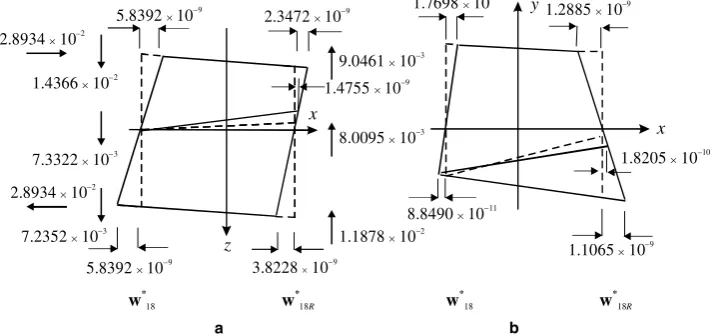
Fig. 9. Principal vectorw
17for shearing force and bending moment in the,xy-plane: (a) and (b) show the displacement and force components in thexy- andxz-planes. respectively.
2.8934 10× –2
1.7698 10× –10
w*
18
5.8392 10× –9
z
x
x y
5.8392 10× –9 2.8934 10× –2
2.3472 10× –9
1.4755 10× –9
3.8228 10× –9
a b
8.8490 10× –11
1.2885 10× –9
1.8205 10× –10
1.1065 10× –9 1.4366 10× –2
7.3322 10× –3
7.2352 10× –3
9.0461 10× –3
8.0095 10× –3
1.1878 10× –2
w*
18R w
*
18 w
*
18R
Fig. 10. Principal vectorw
[image:16.544.91.454.327.495.2]x y
2.6496 10X –9
4.2041 10X –9 6.9167 10X –10
a
5.2991 10X –9
4.8958 10X –9
x y
7.2169 10X –10
1.1451 10X –9 1.8840 10X –10
b
1.4434 10X –9
[image:17.544.117.435.98.234.2]1.3335 10X –9
Fig. 11. Decomposition of the displacements in thexy-plane ofFig. 9: (a) shows the shear angle due to shearing force and (b) shows the bending curvature due to bending moment.
z
x
a 6.8056 10X –10
6.8056 10X –10
3.0073 10X –10 4.7839 10X –10
7.7912 10X –10
z
x
b 5.2729 10X –10
5.2729 10X –10
2.3300 10X –10 3.7065 10X –10
[image:17.544.125.429.288.431.2]6.0365 10X –9
Fig. 12. Decomposition of the displacements in thexz-plane ofFig. 9: (a) shows the bending curvature coupled with the shear angle in the,xz-plane due to shearing force and (b) shows the shear angle coupled with the bending curvature in the,xz-plane due to bending moment.
4.5892 10X –9
z
x
4.5892 10X –9
3.2259 10X –9
5.2538 10X –9
a b
1.25 10X –9
z
x
1.25 10X –9
8.7867 10X –10
1.4310 10X –9 2.0279 10X –9 5.5236 10X –10
[image:17.544.123.427.494.637.2]x y
6.0886 10X –10
3.0443 10X –10
5.6252 10X –10
7.9472 10X –11
4.8304 10X –10
x y
7.8584 10X –10
3.9292 10X –10
7.2602 10X –9
1.0257 10X –10
6.2345 10X –10
[image:18.544.112.429.94.232.2]a b
Fig. 14. Decomposition of the displacements in thexy-plane ofFig. 10: (a) shows the bending curvature coupled with the shear angle in thexy-plane due to shearing force and (b) shows the shear angle coupled with the bending curvature in thexy-plane due to bending moment.
y
z y
z
b a
9.3197 10X –10
3.5904 10X –10
2.3190 10X –10 7.1807 10X –10
6.3903 10X –10
2.3390 10X –10 1.7123 10X –10
1.4361 10X –9 4.6780 10X
9 – y′
[image:18.544.106.437.298.437.2]z′
Fig. 15. Displacements in the y-direction for the principal vectorw
17 on the left-hand (a) and right-hand (b) sides of the cell, respectively.
y
z y
z
b a
1.0771 10X –9 2.3390 10X
10 – 1.6500 10X –9
5.0417 10X –10 7.1807 10X –10
6.3903 10X –9
1.7123 10X –10 4.6780 10X –10
Fig. 16. Displacements in thez-direction for the principal vector w
[image:18.544.120.423.495.637.2]are exactly one half of those associated withw15, as one might expect: for a continuum, a shearing force
induces a bending moment which varies linearly along the length, whose effect should be one-half that of a pure moment, the latter being constant along the length of the cell. These secondary effects become evident within a cell of finite length, but are not included within the coupled constitutive relationships, such as Eq. (57), which is applicable to a continuum element of infinitesimal length.
FromFigs. 11(a) and 13(a), the cross-sectional rotation on either end of the cell in the two planes, as
wz¼2.649610
9
H=3 ¼2.677510 8
; wy ¼4.589210
9
L=2 ¼2.677510 8
. ð51a;bÞ
Moreover, they- andz-direction displacements within vectorsw
17andw17R, andw18andw18Rsuggests a
shift of the centre of area on the left-hand side of the cell for both, as shown inFigs. 15 and 16, respectively. The centre line slope rotations within the two shear vectors can then be determined as
ov ox¼
7.18071010
0.3428 ¼2.094710
9; ow
ox¼
7.18071010
0.3428 ¼2.094710
9; ð
52a;bÞ
so the shear angles in the two planes are
cxy¼wzov=ox¼2.4680108; cxz¼wyow=ox¼2.4680108. ð53a;bÞ
From the above discussion on the bending moment vectors, it is known that a pure bending moment produces a bending curvature in the principal plane and a coupled shear deformation in the perpendicular plane. According to the reciprocal theorem, when the cell is subject to a shear, it should result in a shear deformation in the principal plane, coupled with a bending curvature in the perpendicular plane; fromFigs.
12(a) and 14(a), these two coupled bending curvatures are, respectively
1 Rz
¼6.805610
10
L=2L=2 ¼2.316610 8
m1; 1
Ry
¼3.929210
10
H=3L=2 ¼2.316610 8
m1. ð54a;bÞ
The secondary bending curvatures produced by the bending momentsMzand Myapplied on the left-hand side of the cell, vectors w17 andw18, but regarded as being linearly distributed along the cell from the left-side to the right which, fromFigs. 11(b) and 13(b), are
1 R0y ¼
7.21691010
H=3L=2 ¼4.254910 8
m1; 1
R0z¼
1.25109
L=2L=2 ¼4.254910 8
m1. ð55a;bÞ
From Figs. 12(b) and 14(b), the secondary coupled shear angles due to these bending moments in the
perpendicular planes are
c0xy¼5.272910
9
L=2 ¼3.076410 9;
c0xz¼3.044310
10
H=3 ¼3.076410 9
. ð56a;bÞ
As presaged above, the bending curvatures and shear angles obtained in Eqs.(55) and (56)are exactly one-half of those obtained in Eqs. (44) and (45), respectively.
The absence of bending–bending coupling for the example structure suggests that any proposed equiv-alent continuum coupling involving bending and shear will not be typical of a pre-twisted structure; indeed, the coupling appears to be closer to that of an asymmetric structure based upon aNASAdeployable frame-work treated by Stephen and Zhang (2004), according to
Qz
Mz
¼ jxzAG Kxz
Kxz EIz
c
xz owz=ox
with an equivalent expression for bending in the perpendicular plane. In order to determine the equiva-lent second moment of area and shear coefficient, it is more convenient to write Eq.(57) in its inverted form
cxz 1=Ry
¼N Qz
Mz
. ð58Þ
whereNis the compliance matrix
N¼ n11 n12
n21 n22
¼ jxzAG Kxz
Kxz EIz
1
. ð59Þ
From the bending vector in the xy-plane, w15, one has Mz= 9.9185·10
3
Nm, Qz= 0, 1/Ry= 8.5098·10
8
m1,cxz= 6.1527·10
9
, and substituting into Eq.(59)gives
n12¼
cxz Mz
¼6.2033107; n22¼
1=Ry Mz
¼8.5797106. ð60a;bÞ
From the shear vector in the xz-plane w18, one has Mz= 0 Nm, Qz= 2.8934·102 N, 1/Ry= 2.3166·108m1,cxz= 2.4680·108, and from Eq.(59)
n11¼
cxz
Qz¼8.529810 7; n
21¼
1=Ry
Qz ¼8.006410 7
. ð61a;bÞ
Inversion of the matrix N gives
jxzAG Kxz Kxz EIz
¼ n11 n12
n21 n22
1
¼ 1.257710
6
9.0935104
1.1737105 1.2504105
" #
; ð62Þ
from which the equivalent second moment of area is Iz= 1.7863· 106m4, and shear coefficient jxz= 0.4134. However, Eqs.(60) and (61)indicate unequal coupling coefficients sincen125n21. Therefore,
the coupled equations are modified, to read
Qz
Mz
¼ jxzAG Kxz
Kzx EIz
c
xz owz=ox
; ð63Þ
and the two coupling coefficients areKxz=9.0935·104Nm,Kzx=1.1737·105Nm.
Similarly, from the bending vector in thexz-plane,w16, and the shear vector in thexy-plane,w17, it is
found thatjxy=jxz,Iy=Iz,Kxy=KxzandKyx=Kzx, within the coupled equations
Qy
My
¼ jxyAG Kxy
Kyx EIy
c
xy owy=ox
" #
; ð64Þ
rotation. This could be confirmed, or discounted, by the analysis of a pre-twisted structure having, say, a rectangular cross-section, and will be investigated in further work. Another possibility is a lack of work-conjugacy in relation to moments and rotations, which according to Ritto-Correa and Camotim (2003)
is known to lead to asymmetric tangent matrices in large displacement, small strain analysis. It is also quite possible that the particular way of presenting the moment-shear coupling needs modification for a pre-twisted structure: thus when one calculates the nodal stiffness matrix K, in global coordinates, which is the first step of the analysis procedure, one is relating nodal force and displacement componentson both sidesof the cell. However, in writing constitutive relationships such as those expressed in Eq.(57), moment and shearing force are only explicitly stated for the left-hand side of the cell, consistent with an infinitesimal element, while those on the right-hand are understood; likewise, curvature and shear are interpreted from the rotation of the cross-section on both sides of the cell. For a straight structure this is quite acceptable— for example, moment equilibrium would require that there is an equal but opposite moment on the right-hand side, while cross-sectional rotations are always expressed within a global coordinate system. For the pre-twisted cell, the implied right-hand side moment is only equal and opposite within the global coordinate system, not the local. A further difficulty lies with the cross-sectional rotation, as finite rotations about dif-ferent axes are known not to commute; this problem does not arise in the case of tension–torsion coupling, since the cross-sectional rotation (deformation) does commute with angle of pre-twist, as they are both about the same axis.
The inability to resolve this issue highlights the need for further research in the general area of bending of pre-twisted structures—both for the idealised discrete structure considered here, and for continuum rods, as in a pre-twisted turbine blade. However, one should emphasise that this issue represents a weakness in interpretation and current understanding, not an error in the principal vectors obtained by the eigenanal-ysis described in this paper—these must be correct, otherwise one would not obtain the correct Jordan canonical form.
6. Conclusions
Appendix A. Transformation matrix and Jordan canonical form
V¼
2.6441108 5.9282108 1.6709108 1.5171108 5.9694108 2.6441108
7.8780108
2.2359107
1.3240107 8.6401
108 1.3240
107 1.5472
108
6.3349108
4.6575108 8.6401
108 4.6575
108
2.2359107 9.9900
108
2.6441108 1.5171
108 5.9694
108 5.9282
108
1.6709108
2.6441108
1.5472108 8.6410
108
1.3240107
2.2359107 1.3240
107 7.8782
108
9.9900108
4.6575108
2.2359107 4.6575
108 8.6401
108
6.3349108
2.6441108 4.4111
108
4.2986108
4.4111108
4.2986108
2.6441108
9.4252108
6.8595108 1.3606
107
6.8595108
1.3606107
9.4252108
3.6650108 2.2189107 6.8595108 2.2189107 6.8595108 3.6550108
0 0 0 0 0 0
1=2 pffiffiffi3=2 1=2 pffiffiffi3=2 1=2 1=2
pffiffiffi3=2 1=2 pffiffiffi3=2 1=2 pffiffiffi3=2 pffiffiffi3=2
0 0 0 0 0 0
1=2 pffiffiffi3=2 1=2 pffiffiffi3=2 1=2 1=2
ffiffiffi
3
p
=2 1=2 pffiffiffi3=2 1=2 pffiffiffi3=2 pffiffiffi3=2
0 0 0 0 0 0
1 0 1 0 1 1
0 1 0 1 0 0
1108 0 0 0 0 0
0 8.44171010 8.57108 3.80191011 1108 0
0 1.4621109 4.9479108 6.58511011 0 1108
1108 0 0 0 0 0
0 8.44171010
8.57108 3.8019
1011 1
108 0
0 1.4621109
4.9479108
6.58511011 0 1
108
1108 0 0 0 0 0
0 1.6883109 0
7.60391011 1
108 0
0 0 9.8958108 0 0 1
108
0 7.6469102 0
9.0323103 0 0
0 7.9046103 0 7.4604
103 0 0
0 4.5637103 0 4.3073103 0 0
0 7.6469102 0 9.0323103 0 0
0 7.9046103 0 7.4604103 0 0
0 4.5637103 0 4.3073103 0 0
0 7.6469102 0
9.0323103 0 0
0 0 0 0 0 0
0 9.1274103 0 8.6146
103 0 0
2.8868109 5
109
3.88801010
3.1089109 2.0225
109 5.9385
109
0 0 3.59041010 6.2187
1010
6.31521010
4.64551010
0 0 6.21871010 1.0771
109
1.0938109
8.04621010
2.8868109
5109
2.4980109 1.8911
109 4.1317
109
4.7208109
0 0 3.59041010 6.21871010 8.65471011 7.79191010
0 0 6.21871010 1.0771109 1.49901010 1.3496109
5.7735109 0 2.8868109 1.2177109 6.1542109 1.2177109
0 0 1.4361109 0 1.4361109 6.29281010
0 0 0 0 0 0
0 0 1.6705102 2.8934
102
2.7259103
3.7005102
0 0 3.5656103
2.0586103
5.9174103 1.7786
103
0 0 2.0586103 3.5656
103 1.7787
103
1.3372102
0 0 1.6705102
2.8934102
3.0684102 2.0863
102
0 0 3.5656103
2.0586103
1.3049102 2.3385
103
0 0 2.0586103
3.5656103 2.3385
103
6.2406103
0 0 3.3410102 0 3.3410102 1.6142102
0 0 0 4.1142103 9.9678103 4.1172103
0 0 4.1172103 0 4.1172103 9.3213103
V1G0V=J, whereJis the real Jordan block matrix.
J¼
22.3303 0 0 0 0 0 0 0 0 0 0 0 0 0 0 0 0 0
0 10.0110 10.0110 0 0 0 0 0 0 0 0 0 0 0 0 0 0 0
0 10.0110 10.0110 0 0 0 0 0 0 0 0 0 0 0 0 0 0 0
0 0 0 0.0499 0.0499 0 0 0 0 0 0 0 0 0 0 0 0 0
0 0 0 0.0499 0.0499 0 0 0 0 0 0 0 0 0 0 0 0 0
0 0 0 0 0 0.0448 0 0 0 0 0 0 0 0 0 0 0 0
0 0 0 0 0 0 1 1 0 0 0 0 0 0 0 0 0 0
0 0 0 0 0 0 0 1 0 0 0 0 0 0 0 0 0 0
0 0 0 0 0 0 0 0 1 1 0 0 0 0 0 0 0 0
0 0 0 0 0 0 0 0 0 1 0 0 0 0 0 0 0 0
0 0 0 0 0 0 0 0 0 0 c s c s 0 0 0 0
0 0 0 0 0 0 0 0 0 0 s c s c 0 0 0 0
0 0 0 0 0 0 0 0 0 0 0 0 c s c s 0 0
0 0 0 0 0 0 0 0 0 0 0 0 s c s c 0 0
0 0 0 0 0 0 0 0 0 0 0 0 0 0 c s c s
0 0 0 0 0 0 0 0 0 0 0 0 0 0 s c s c
0 0 0 0 0 0 0 0 0 0 0 0 0 0 0 0 c s
0 0 0 0 0 0 0 0 0 0 0 0 0 0 0 0 s c
2 6 6 6 6 6 6 6 6 6 6 6 6 6 6 6 6 6 6 6 6 6 6 6 6 6 6 6 6 6 6 6 6 6 6 6 6 6 6 6 4 3 7 7 7 7 7 7 7 7 7 7 7 7 7 7 7 7 7 7 7 7 7 7 7 7 7 7 7 7 7 7 7 7 7 7 7 7 7 7 7 5 ;
wherec¼cosa,s¼sina anda=p/8.
Appendix B. Two shear vectors
½w17 w18 ¼
3.5245109 5.7507109
9.31971010 2.91081010
1.6142109 5.04171010 3.2180109 5.9277109
2.13901010 9.52651010 3.70491010 1.6500109
6.7425109 1.7698109
1.4361109 1.32311010
0 0
1.6705103 2.8934102
4.9228103 5.5975105 5.5975105 1.4366102
1.6705102 2.8934102
1.2054102 4.0612103 4.0612103 7.2352103
3.3410102 0
1.1957102 4.1172103 4.1172103 7.3322103
References
Chen, C., 1951. The effect of initial twist on the torsional rigidity of thin prismatical bars and tubular members. In: Proceedings of the First US National Congress of Applied Mechanics. ASME, New York.
Di Prima, R.C., 1959. Coupled torsional and longitudinal vibrations of a thin bar. ASME Journal of Applied Mechanics 26 (4), 510–512.
Goodier, J.N., Griffin, D.S., 1969. Elastic bending of pretwisted bars. International Journal of Solids and Structures 5 (11), 1231–1245. Guglielmino, E., Saccomandi, G., 1996. On the bending of pretwisted bars by a terminal transverse load. International Journal of
Engineering Science 34 (11), 1285–1299.
Kelley, W.G., Peterson, A.C., 2001. Difference equations, second ed. Academic Press, New York.
Krenk, S., 1983a. A linear theory for pretwisted elastic beams. ASME Journal of Applied Mechanics 50 (1), 137–142.
Krenk, S., 1983b. The torsion-extension coupling in pretwisted elastic beams. International Journal of Solids and Structures 19 (1), 67–72.
Okubo, H., 1951. The torsion and stretching of spiral rods (I). Quarterly of Applied Mathematics 9 (3), 263–272. Okubo, H., 1953. The torsion of spiral rods. ASME Journal of Applied Mechanics 20 (2), 273–278.
Okubo, H., 1954. The torsion and stretching of spiral rods (II). Quarterly of Applied Mathematics 11 (4), 488–495.
Pucci, E., Risitano, A., 1996. Bending of a pretwisted bar by terminal transverse load. International Journal of Engineering Science 34 (4), 437–452.
Ritto-Correa, M., Camotim, D., 2003. Work-conjugacy between rotation dependent moments and finite rotations. International Journal of Solids and Structures 40 (11), 2851–2873.
Rosen, A., 1991. Structural and dynamic behaviour of pretwisted rods and beams. ASME Applied Mechanics Reviews 44 (12), 483–515.
Shield, R.T., 1982. Extension and torsion of elastic bars with initial twists. ASME Journal of Applied Mechanics 49 (4), 779–786. Stephen, N.G., Wang, P.J., 1996. On Saint-Venants principle in pin-jointed frameworks. International Journal of Solids and
Structures 33 (1), 79–97.
Stephen, N.G., Zhang, Y., 2004. Eigenanalysis and continuum modelling of an asymmetric beam-like repetitive structure. International Journal of Mechanical Sciences 46 (8), 1213–1231.