© 2015Journal of ISOSS 1 2015 Vol. 1(1), 01-11
IMPROVING STATISTICAL INFERENCE WITH UNCERTAIN NON-SAMPLE PRIOR INFORMATION
ShahjahanKhan1, Muhammed Ashraf Memon2 Budi Pratikno3and Rossita M Yunus4
Email address of corresponding author: [email protected]
1School of Agric., Comput. and Environmental Sciences
International Centre for Applied Climate Sciences, Centre for Health Sciences Research, University of Southern Queensland, Toowoomba, Australia
2Sunnybank Obesity Centre &SEQS, Suite 9, 259 McCullough Street Sunnybank, Queensland, AUSTRALIA Mayne Medical School, University of Queensland, Australia Faculty of Health Sciences & Medicine, Bond University, Australia
3Department of Mathematics and Natural Science Jenderal Soedirman University, Purwokerto, Indonesia
4Institute of Mathematical Sciences, University of Malaya Kuala Lumpur, Malaysia
ABSTRACT
In the classical inference, the observed sample data is the only source of information. The Bayesian inferential methods assume prior distribution of the underlying model parameters to combine with sample data. Often non-sample prior information (NSPI) on the value of the model parameters is available from previous studies or expert knowledge which could be used along with the sample data to improve the quality of statistical inference. Obviously the NSPI is not always correct and hence there is uncertainty in the suspected value of the parameter. Any such uncertainty can be removed by conducting an appropriate statistical test, and the quality of statistical inference can be improved by including the outcome of the test in the inferential procedure. This paper provides the underlying methodology to illustrate the process and include an example to demonstrate its application.
KEYWORDS AND PHRASES: Regression model; uncertain non-sample prior information; restricted, preliminary test and shrinkage estimators; bias, relative efficiency, M and score tests, testing after pre-test, power of tests, correlated non-central bivariate chi-square distribution.
1 INTRODUCTION
Statistical inference uses both sample and non-sample information. Classical inference uses only the sample data for estimation and test of hypotheses. Bayesian methods uses sample data and prior distribution of the model parameters. The notion of inclusion of non-sample prior information (NSPI) on the value of model parameters has been introduced to `improve' the quality of statistical inference. The natural expectation is that the inclusion of additional information would result in a better estimator and test with relevant statistical properties. In some cases this may be true, but in many other cases the risk of worse consequences can not be ruled out.
A number of estimators have been introduced in the literature that uses NSPI and, under particular situation, over performs the traditional exclusive sample information based unbiased estimators when judged by criteria such as the mean square error and squared error loss function.
In many studies the researchers estimate the slope parameter of the regression model. However, the estimation of the intercept parameter is more difficult than that of the slope parameter. This is because the estimator of the slope parameter is required in the estimation of the intercept parameter. Khan et al. (2002) studied the improved estimation of the slope parameter for the linear regression model. They introduced the coefficient of distrust on the belief of the null hypothesis, and incorporated this coefficient in the definition and analysis of the estimators.
In recent time (eg Khan and Pratikno, 2013; Yunus and Khan, 2008, 2010, 2011a,b) several studies used NSPI on the slope of a regression model to test the intercept parameter. Yunus (2010) applied the NSPI in the testing regime using M-test along the line of Humber's M-estimation. Pratikno (2012) studied the parametric test for the intercept parameter using NSPI information on the slope of different regression models.
In general the NSPI on the slope is uncertain and may fall into one of the following three categories: (i) unspecified, no information available, (ii) specified, correct value known, and (iii) specified with uncertainty.
This paper provides alternative estimators and tests of the intercept parameter when NSPI on the slope of the simple linear regression model is available.This include the unrestricted (UE), restricted (RE), preliminary test (PTE) estimators as well as the unrestricted (UT), restricted (RT) and pre-test (PTT) tests of the intercept parameter. Statistical properties of these estimators and tests are investigated both analytically and graphically. Motivation for a real life application of test for the intercept is found in Kent (2009).
The next section introduces the model and definition of the unrestricted estimators of 2
and
.The three alternative estimators are defined in Section3 along with their properties. The three tests and their power analyses are provided in Section 4. Some concluding remarks are given in section 5.
2 THE MODEL AND SOME PRELIMINARIES
The n independently and identically distributed responses from a linear regression model can be expressed by the equation
1n
y x e, (2.1)
where y and x are the column vectors of response and explanatory variables respectively,
1n (1, ,1)- a vector of n-tuple of 1's, and are the unknown intercept and slope
parameters respectively and e( ,e1,en) is a vector of errors with independent
components which is distributed asNn(0,2In). So that E e( ) 0 and
2
( ) n
E ee I
where 2 is the variance of each of the error component in eand In is the identity matrix of order n.
Assume that uncertain NSPI on the value of is available, either from previous study or from practical experience of the researchers or experts. Let the NSPI be expressed in the form of H0: 0 which may be true, but not sure. We wish to incorporate both the sample information and the uncertain NSPI in estimating and testing the intercept. Following Khan et al (2002) we assign a coefficient of distrust, 0 d 1, for the NSPI, that represents the degree of distrust in the null hypothesis.
The unrestricted mle of the slopeand intercept are given by 1
(xx) x y and y x,
(2.2)
where
1
1 n j j
x x
n
and1 1 n
j j
y y
n
. The mle of 2is Sn*2 1(y yˆ) (y yˆ),n
where
ˆ 1n
y x. This estimator is biased for2. However, 2 1 ( ˆ) ( ˆ)
2 n
S y y y y
n
is
unbiased for2. To remove the uncertainty from the NSPI, we perform an appropriate statistical test on H0: 0against Ha: 0. Here the appropriate test is given by
1 1 2
0
( ).
n xx
LS S Under theHa,L, follows a non-central Student-t distribution with (n 2)
df and non-centrality parameter 2 2Sxx( 0)2
.
3 ALTERNATIVE ESTIMATORS OF INTERCEPT
3.1 The Estimators
The UE, RE and PTE of are given by UE
y x
(3.1)
RE
ˆ ( )d d (1 d) ,ˆ 0 d 1
(3.2)
PTE RE
ˆ ( )d ˆ ( ) (d I F F ) I F
(
F)
(1 ) ( )
x d I F F
. (3.3)
The bias of the estimators are obtained as (cf Hoque et al. 2006) UE
1[ ( )] 0
B d (3.4)
RE 1/2
2[ˆ ( )] xx (1 )
B d S x d (3.5)
PTE 1 2
3[ˆ ( )] (1 ) 3,
(
3 ;)
,B d d x G F (3.6)
where 1 2
2 , (·; ) n n
G is the c.d.f. of a non-central F-distribution with ( ,n n1 2)df and non-centrality parameter 2 which is the departure constant from the null-hypothesis. Among the three estimators, the UE is the only unbiased estimator.
The mean squared errors (MSE) of the estimators become
UE 2
1[ ]0
M H (3.7)
RE 2 2 2 1 2 2
2[ˆ ( )] (1 ) xx
M d d H d S x (3.8)
PTE 2 1 2 2 2 1 2
3[ˆ ( )] xx 2(1 ) 3,v
(
3 ;)
M d HS x d G F
2 1 2 2 1 2
5, 3,
(1 d )G v
(
5 F ;)
(1 d )G v(
3 F ;)
,
(3.9)
whereH
n1S xxx1 2
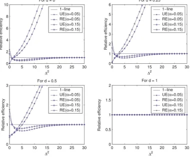
.The relative efficiency of the PTE relative to the UE and RE is 1
PTE UE 1 2 2 2
ˆ
RE
[
( ) :d]
H H S xxx g( )
(3.10)
and
PTE RE 2 2 2 1 2
1 1 2 2
ˆ ˆ
RE ( ) : ( ) (1 )
( )
[
]
xxxx
d d d H d S x
H S x g
(3.11)
respectively, where
2 2 1 2 2 1 2
3, 5,
( )
{
2(1 ) v(
3 ;)
(1 ) v(
5 ;)}
g d G F d G F
2 1 2
3,
(1 d )G v
(
3 F ;)
.
(3.12)
Figure 1: Graph of the relative efficiency of PTE relative to UE and RE against 2.
4 THREE TESTS OF INTERCEPT
In this section we define three alternative tests of the intercept and investigate their properties.
To remove the uncertainty in the NSPI on, we perform a pretest (PT) on *
0: 0
H before testing on the intercept. Let PT be the test function for pretesting *
0
H : 0 (a suspected constant) againstH*a: 0. If the
* 0
4.1 Three Test Statistics
Under the three scenarios on the UT, RT and PTT for testing H0: 0 (known constant) against Ha: 0 are defined as follows:
(i) UT= test function and TUT is the test statistic when is unspecified, (ii) RT= test function and TRT is the test statistic when 0 is specified and (iii) PTT= test function and TPTT is the test statistic following a PT on H0* when
0
is uncertain.
The test statistics are obtained as
1
2 1 2 2
0 0
( ) / ( ) ( ) (1 )
UT
n xx
T SE n Y X S S nX
(4.1)
1 0
0 0 1
ˆ ( ) ˆ ˆ ( ) / ( )% ( ) ~ , / RT y n y
T SE s n Y t
s n (4.2)
whereTUT ~tn2, and
2 2 1 1 ( ) 1 n y i i
s Y Y
n
. Let us choose a positive number, (0 1, for j=1, 2,3)
j j
then let 2,
j n
t be such that
1
2, ˆ 0 1, UT
n
P T t U
1, 2 0
2ˆ RT
n
P T t U , and
2, 3 0
3 0 0ˆ .Then,the PTT fortesting :
PT n
P T t U H when 0is uncertain is given by the test function
33 21
PT RT
n-2, n-1,
PT UT
n-2, n-2,
1, if T t , T t
or T t , T t ;
0, otherwise. PTT (4.3)
4.2 Properties of the Tests
Let {Kn} be a sequence of alternative hypotheses defined as
1/ 2 1 2 0 0 : ( , ) , , n K n n n (4.4)
where ( 1, 2) is a vector of fixed real numbers and is the true value of the intercept. Under Kn, ( 0) 0and underH0, ( 0) 0.
Student-t distribution with (n-2)df and correlation coefficient with 1 3
( 2)
( , )
( 4)
UT PT n
Cov T T
n
(cf., Kotz and Nadarajah, 2004). The power functions of the tests are given by
1, 2 ˆ
( ) ( )
UT UT
n n
P T t UK
1
1
1 , 2 1
1 P TUT t n k
(4.5)
1, 1
ˆ ( )
RT RT
n n
P T t UK
2
1 2 , 1 ( 0) ( 0)
RT
n y
P T t n X s
2
1
2 , 1 1 2
1 P TRT t n Xsy
(4.6)
2, 3 1, 2
( ) ,
PTT PT RT
n n
P T t T t
3 1
2, , 2,
PT UT
n n
P T t T t
3 2
1
2 2 1
10 n 2, 2 xx[ n ] , ,n 1 y ( 1 2 ), 0
d t S S n t s X
3 1 1
2 2 1
2 n 2, 2 xx[ n ] , ,n 2 1 , 0 , d t S S n t k
3 2 1 2
10 2, 2 , 1
( ) % 0 , , xx n n y n S X
d t t
s S n 3 1 1
2 2, 2 , , 2 1 , 0 ,
xx
n n
n S
d t t k
S n (4.7)
wherek Sn (1 nX S2 xx1),d10andd2
are bivariate Student's t probability integrals. Here d10 is defined as d10
a cf t( PT,tRT)dtPTdtRT,3 2
1 2
2, 2 and 1, ,
xx
n n
y n
S X
a t c t
s S n and 2
d is defined as
2
2 2 2
2 2
2 2
( 2 )
2
( , , ) 1 ,
(1 )
1 2
a b
x y xy
d a b dxdy
n
in which 1 1 is the correlation coefficient between the TUT, TPT and 1,n 2 1/
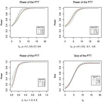
The power curves of the PTT for different values of is provided in Figure 3.
Figure 3: The power curve of the PTT against 2, and its power and size curves against .
5 CONCLUDING REMARKS
In practice, the NSPI is obtained from expert knowledge or previous studies, and hence the value of the parameter available from prior information is expected to be close to its true value and the degree of distrust on the null hypothesis is very likely to be close to 0.
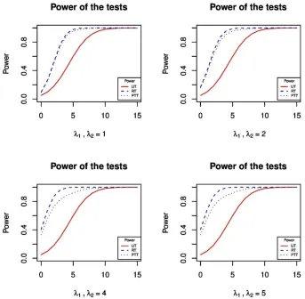
Of the three tests, the RT has the maximum power and size, and the UT has minimum power and size. So none of them is achieving the highest power and lowest size. But the PTT protects against maximum size of the RT and minimum power of the UT. As
2 0
the difference between the power of the PTT and RT diminishes for all values of 2 0
. That its, if the NSPI is accurate the power of the PTT is about the same as that of the RT. Moreover, the power of the PTT gets closer to that of the RT as 1. If
1
then the power of the PTT matches with that of the RT. Thus if there is a high (near 1) correlation between the TUTandTPTthe power of the PTT is very close to that of the RT.
ACKNOWLEDGEMENT
The authors are thankful to the referees and editors for their valuable suggestions. A draft version of this paper was presented at the 13th Islamic Countries Conference on Statistical Sciences (ICCS-13) in Bogor, Indonesia,
REFERENCES
1. Bancroft, T.A. (1944). On biases in estimation due to the useof the preliminary tests of significance. Annals ofMathematical Statistics, 15, 190-204.
2. Chiou, P., and Saleh, A K Md E. (2002). Preliminary test confidence sets for the mean of a multivariate normaldistribution. Journal of Propagation in Probability and Statistics, 2, 177-189.
3. Han, C.P., and Bancroft, T.A. (1968). On pooling means whenvariance is unknown. Journal of American Statistical Association, 63, 1333-1342.
4. Hoque, Z., Khan, S., and Wesolowski, J. (2009). Performance of preliminary test estimator under linex loss function. Communications in Statistics: Theory and Methods, 38 (2). pp. 252-261.
5. Judge, G.G., and Bock, M.E. (1978). The Statistical Implications of Pre-test and Stein-rule Estimators inEconometrics. North-Holland, New York.
6. Kent, R. (2009). Energy miser-know your plants energy, Fingerprint (accesed 23 May 2011). {URL}:http://www.ptonline.com/articles/know-your-plants-energy-fingerprint.
7. Khan, S. (2008). Shrinkage estimators of intercept parameters of two simple regression models with suspected equal slopes. Communications in Statistics - Theory and Methods, 37, 247-260.
8. Khan, S. (2003). Estimation of the parameters of two parallel regression lines under uncertain prior information. Biometrical Journal, 44, 73-90.
9. Khan, S. (1998). On the estimation of the mean vector of Student-t population with uncertain prior information. Pakistan Journal of Statistics, 14, 161-175.
10. Khan, S., Hoque, Z., and Saleh, A K Md E. (2005). Estimation of the intercept parameter for linear regression model with uncertain non-sample prior information. Statistical Papers, 46 (3). pp. 379-395
12. Khan, S. and Pratikno, B. (2013) Testing base load with non-sample prior information on process load. Statistical Papers. 54(3), 605-617
13. Khan, S., and Saleh, A K Md E. (2001). On the comparison of the pre-test and shrinkage estimators for the univariate normal mean. Statistical Papers, 42(4), 451-473.
14. Khan, S., and Saleh, A K Md E. (1997). Shrinkage pre-test estimator of the intercept parameter for a regression model with multivariate Student-t errors. Biometrical Journal, 39, 1-17.
15. Pratikno, B. (2012). Test of hypotheses for linear regression models with non-sample prior information. Unpublished PhD Thesis, University of Southern Queensland, Australia
16. Saleh, A K Md E. (2006). Theory of Preliminary Test Stein-Type Estimation with Application, Wiley, New York.
17. Saleh, A K Md E., and Sen, P K. (1985). Shrinkage least squares estimation in a general multivariate linear model. Proceedings of the Fifth Pannonian Symposium on MathematicalStatistics, 307-325.
18. Saleh, A K Md E., and Sen, P K. (1978). Nonparametric estimation of location parameter after a preliminary test onregression. Annals of Statistics, 6, 154-168. 19. Sclove, S.L., Morris,. andRao, C.R. (1972). Non-optimality of preliminary-test
estimators for the mean of amultivariate normal distribution.Ann. Math. Statist., 43, 1481-1490.
20.Stein, C. (1956). Inadmissibility of the usual estimator forthe mean of a multivariate normal distribution, Proceedingsof the Third Berkeley Symposium on Math. Statist. AndProbability, University of California Press, Berkeley, 1,197-206.
21. Stein, C. (1981). Estimation of the mean of a multivariate normal distribution. Annals of Statistics 9,1135--1151.
22. Tamura, R. (1965). Nonparametric inferences with a preliminary test. Bull. Math. Stat. 11, 38-61.
23. Yunus, R. M. (2010). Increasing power of M-test through pre-testing. Unpublished PhD Thesis, University of Southern Queensland, Australia.
24.Yunus, R. M., and Khan, S. (2008). Test for intercept after pre-testing on slope - a robust method. In: 9th Islamic Countries Conference on Statistical Sciences (ICCS-IX): Statistics in the Contemporary World - Theories, Methods and Applications, 81-90.
25. Yunus, R. M., and Khan, S. (2011a). Increasing power of the test through pre-test - a robustmethod. Communications in Statistics-Theory and Methods, 40, 581-597. 26. Yunus, R. M., and Khan, S. (2011b). M-tests for multivariate regression model.