Advance Access publication 2017 June 9
A comparison of shock-cloud and wind-cloud interactions: the longer
survival of clouds in winds
K. J. A. Goldsmith
‹and J. M. Pittard
School of Physics and Astronomy, University of Leeds, Woodhouse Lane, Leeds LS2 9JT, UK
Accepted 2017 June 7. Received 2017 June 5; in original form 2017 January 18
A B S T R A C T
The interaction of a hot, high-velocity wind with a cold, dense molecular cloud has often been assumed to resemble the evolution of a cloud embedded in a post-shock flow. However, no direct comparative study of these two processes currently exists in the literature. We present 2D adiabatic hydrodynamical simulations of the interaction of a Mach 10 shock with a cloud of density contrastχ=10 and compare our results with those of a commensurate wind-cloud simulation. We then investigate the effect of varying the wind velocity, effectively altering the wind Mach numberMwind, on the cloud’s evolution. We find that there are significant
differences between the two processes: 1) the transmitted shock is much flatter in the shock-cloud interaction; 2) a low-pressure region in the wind-shock-cloud case deflects the flow around the edge of the cloud in a different manner to the shock-cloud case; 3) there is far more axial compression of the cloud in the case of the shock. AsMwindincreases, the normalized rate of
mixing is reduced. Clouds in winds with higherMwindalso do not experience a transmitted
shock through the cloud’s rear and are more compressed axially. In contrast with shock-cloud simulations, the cloud mixing time normalized by the cloud-crushing time-scaletccincreases
for increasingMwind until it plateaus (attmix25tcc) at highMwind, thus demonstrating the
expected Mach scaling. In addition, clouds in high Mach number winds are able to survive for long durations and are capable of being moved considerable distances.
Key words: hydrodynamics – shock waves – stars: winds, outflows – ISM: clouds – ISM: kinematics and dynamics.
1 I N T R O D U C T I O N
The flow of hot, high velocity gas through the interstellar medium (ISM) is known to play an important local role in star formation, and on much larger scales the formation and evolution of galaxies. The interaction of such flows with much cooler, dense clumps of gas (i.e. ‘clouds’) can lead to the entrainment of cloud material. This shapes the morphology of the cloud and can ultimately cause the destruction of the cloud, altering the gas dynamics of the ISM (see Goldsmith & Pittard2016for cases where the cloud is not destroyed on the usual dynamical time-scales). These interactions can inform our understanding of the nature of the ISM (see e.g. Elmegreen & Scalo2004; Mac Low & Klessen2004; Scalo & Elmegreen2004; McKee & Ostriker2007; Hennebelle & Falgarone2012; Padoan et al. 2014), galaxy formation (e.g. Sales et al. 2010), and the evolution of supernova remnants (SNRs) and other diffuse sources (e.g. McKee & Ostriker1977; Cowie, McKee & Ostriker 1981; White & Long1991; Dyson, Arthur & Hartquist2002; Pittard et al.
2003).
E-mail:[email protected]
Observational studies have provided evidence of the interaction of hot flows with molecular clouds (e.g. Koo et al.2001; Westmo-quette et al.2010). High velocity winds and shocks in regions of star formation are capable of strongly affecting molecular clouds. For example, the B59 filament in the Pipe nebula is thought to be undergoing distortion by a wind (Peretto et al.2012) and molecu-lar cloud complexes in the Cygnus X region are being shaped by winds and radiation (Schneider et al.2006), whilst winds lead to the disruption, fragmentation or dispersion of clouds such as the Rosette molecular cloud (Bruhweiler et al.2010, see also Rogers & Pittard2013and Wareing, Pittard & Falle2017for relevant nu-merical studies). Another effect of the interaction of a flow with a dense cloud is the entrainment of the cloud into the flow and acceleration of cloud material towards the flow’s velocity. Several studies have revealed large outflow velocities from rapidly star-forming galaxies (e.g. Heckman et al.2000; Pettini et al.2001; Rupke, Veilleux & Sanders2002; Martin2005; Martin et al.2012) and clouds have been typically observed at distances of a few kpc from the driving region (e.g. Soto & Martin 2012). How-ever, it has proved less easy to reconcile observations that clouds can travel distances on the order of 100 kpc without being de-stroyed (e.g. Turner et al.2014) by flows of such high velocity, and
C
2428
K. J. A. Goldsmith and J. M. Pittard
Scannapieco & Br¨uggen (2015) determined that in order to achieve these velocities clouds would need to be the size of entire galaxies. In addition to observations, shock-cloud interactions, in particu-lar, have also been studied experimentally. For instance, the evolu-tion of a sphere of dense material interacting with a laser-induced shock has been probed by X-ray radiography (Klein et al.2003; Hansen et al.2007).
The idealized case of a shock striking a spherical cloud was ini-tially investigated numerically in the 1970s. Klein, McKee & Colella (1994) provided the first detailed 2D study of such interactions and examined the effects of varying the shock Mach number,M, and cloud density contrast,χ, on the evolution of the cloud. Since then, numerous studies have been conducted in both 2D and 3D, many of which have included additional processes such as radiative cooling (e.g. Mellema, Kurk & R¨ottgering2002; Fragile et al.2004; Yirak, Frank & Cunningham2010), thermal conduction (e.g. Orlando et al.
2005,2008), magnetic fields (e.g. Mac Low et al.1994; Shin-S., Stone & Snyder 2008; Johansson & Ziegler 2013; Li, Frank & Blackman 2013), turbulence (e.g. Pittard et al. 2009; Pittard, Hartquist & Falle 2010; Pittard & Parkin 2016; Goodson et al.
2017), and multiple clouds (e.g. Poludnenko, Frank & Blackman
2002; Al¯uzas et al.2012,2014). Other numerical studies have con-sidered how the nature of the interaction changes when the cloud is non-spherical (e.g. Xu & Stone1995; Pittard & Goldsmith2016; Goldsmith & Pittard2016).
In addition to the large body of literature concerning shock-cloud interactions, many computational studies over the last two decades have considered the particular case of a hot, tenuous wind interacting with a cool, dense cloud (e.g. Klein et al.1994briefly addressed the simple case of the 2D adiabatic interaction of a spherical cloud with a wind where the initial shock has been removed i.e. a cloud embedded within a post-shock flow). These studies have tended to focus on scenarios involving radiative cooling (see e.g. Marcolini et al.2005; Pittard et al.2005; Raga, Steffen & Gonz´alez2005; Raga et al.2007; Cooper et al.2008,2009; Scannapieco & Br¨uggen
2015) or magnetic fields (e.g. Gregori et al.1999,2000; McCourt et al.2015; Banda-Barrag´an et al.2016).
The coupling of stellar feedback processes (winds, shocks from SNRs, etc.) with clouds can produce superficially similar dynamical effects. Pittard et al. (2009) noted that clouds with a high density contrast were able to survive the passage of a shock and would then be immersed in a post-shock flow that would resemble a wind with the same Mach number. Since the simulation of a hot, high-velocity wind can therefore be thought of as resembling a post-shock flow, many wind-cloud papers are highly pertinent to the shock-cloud scenario and vice-versa. Although both wind-cloud and shock-cloud interactions have been well studied, there exists, to our knowledge, no direct comparison of the two processes in the literature. This, therefore, forms the motivation for our current work. In this paper we investigate a 2D hydrodynamical, adiabatic wind-cloud interaction and compare our results to those of a shock-wind-cloud simulation using similar initial parameters. We then incrementally increase the velocity of the wind to increase its effective Mach number and explore the impact this has on the evolution of the cloud. A future paper will extend the analysis to include clouds with increased density contrasts.
The outline of this paper is as follows. In Section 2, we intro-duce our numerical method and initial conditions. In Section 3, we present the results of our simulations. A brief discussion of the relevance of our work in terms of Mach scaling and the longevity of the cloud can be found in Section 4. Section 5 summarises and concludes.
2 T H E N U M E R I C A L S E T U P
The Eulerian equations of inviscid flow are solved numerically for the conservation of mass, momentum and energy:
∂ρ
∂t + ∇ ·(ρu)=0, (1)
∂ρu
∂t + ∇ ·(ρuu)+ ∇P =0, (2)
∂E
∂t + ∇ ·[(E+P)u]=0, (3) respectively, whereρis the mass density,uis the velocity,Pis the thermal pressure,γis the ratio of specific heat capacities, and
E= γP− 1+
1 2ρu
2
(4)
is the total energy density. In this study we limit ourselves to a purely hydrodynamical scenario, ignoring the effects of thermal conduc-tion, radiative cooling, magnetic fields, background turbulence and self-gravity. All computations were computed for an adiabatic, ideal gas, withγ =5/3. The calculations in this study were performed using theMGhydrodynamical code which uses adaptive mesh re-finement. The code solves a Riemann problem at each cell interface in order to determine the conserved fluxes for the time update, using piecewise linear cell interpolation. A linear solver is used in most instances, with the code switching to an exact solver where there is a large difference between the two states (Falle1991). The scheme is second-order accurate in space and time.
A hierarchy ofngrid levels,G0···Gn−1, is used and two grids (G0andG1) cover the entire computational domain, with finer grids being added where needed and removed where they are not. The amount of refinement is increased at points in the mesh where shocks or discontinuities exist, i.e. where the variables associated with the fluid show steep gradients. At these points, the number of computational grid cells produced by the previous level is increased by a factor of two in each spatial direction. Thus, fine grids are only utilized in regions where the flow is highly variable, with much coarser grids used where the flow is relatively uniform. Refinement and derefinement are performed on a cell-by-cell basis and are controlled by the differences in the solutions on the coarser grids at any point in space. Refinement occurs when there is a difference of more than 1 per cent between a conserved variable in the finest grid and its projection/prolongation from a grid one level down. If the difference in the two preceding levels falls to below 1 per cent, the cell is derefined. The time-step on gridGn ist
0/2n, where t0is the time-step on gridG0. The effective resolution is taken to be the resolution of the finest grid and is given asRcr, where ‘cr’ is the number of cells per cloud radius in the finest grid. Each of our simulations was performed at an effective resolution ofR128. All length scales are measured in units of the cloud radius, rc, whererc=1, velocities are measured in units of the shock velocity through the ambient medium,vb, the unit of density is taken to be
the density of the ambient medium,ρamb, and the unit of pressure is the ambient pressure,Pamb. We impose no inherent scale on our simulations. Thus, our calculations can easily be applied to any physical scale required.
2.1 Initial conditions
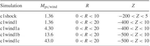
Table 1. The grid extent for each of the simulations (see Section 3 for the model naming convention).Mps/windrefers to the effective Mach number of
the post-shock flow/wind. The unit of length is the initial cloud radius,rc.
Simulation Mps/wind R Z
c1shock 1.36 0<R<10 −200<Z<5 c1wind1 1.36 0<R<20 −400<Z<10 c1wind1a 4.30 0<R<20 −400<Z<10 c1wind1b 13.6 0<R<20 −500<Z<10 c1wind1c 43.0 0<R<20 −500<Z<10
contrastχ=10 initially centred on the grid originr,z=(0, 0) on a two-dimensional RZ cylindrically symmetric grid. We retain these parameters for the simulations of a wind-cloud interaction but fill the entire domain external to the cloud with the post-shock flow, which mimics a mildly supersonic wind. We explore the effect of increasing the velocity of the flow,vps/wind– effectively increasing the Mach number of the wind – on the evolution of the cloud. The numerical domain is set to be large enough so that the cloud is sufficiently mixed into either the post-shock flow or wind before reaching the edge of the grid. Table 1details the grid extent for each of the simulations.
The simulated cloud is assumed to have sharp edges, which max-imises the growth of Kelvin-Helmholtz (KH) instabilities and sets a lower limit to the cloud’s lifetime (see e.g. Nakamura et al.2006; Pittard & Parkin2016). The shock-cloud simulation is described by the sonic Mach number of the shock,Mshock, and the density contrast between the cloud and the stationary ambient medium,χ. The cloud is initially in pressure equilibrium with its surroundings. The Mach number of the post-shock flow/wind is defined as
Mps/wind= vps/wind cps/wind
, (5)
where cps/wind, the adiabatic sound speed of the post-shock
flow/wind, is given bycps/wind=
γPps/wind
ρps/wind.
For theM=10 shock-cloud simulation, the post-shock density, pressure and velocity areρps/ρamb= 3.9,Pps/Pamb =124.8 and vps/vb=0.74, respectively. In modelc1wind1, the cloud is
com-pletely surrounded by the post-shock flow conditions used in model
c1shock. It thus interacts with a flow which has the same density, pressure and velocity as the post-shock material in modelc1shock. The cloud is thus under-pressure compared to the surrounding flow, but at exactly the same pressure as in the shock-cloud simulation.1 The Mach number of this flow/wind (with respect to the cloud) is
Mps/wind=1.36. In the remaining wind models, the velocity of the wind is increased by factors of√10,√100 and√1000 in models
c1wind1a,c1wind1b, andc1wind1c, respectively. This results in an increase in the Mach number of the wind. Values forMwindfor each of these simulations are given in Table1. However, the sound speed of the wind remains the same throughout.
2.2 Global quantities
Various diagnostic quantities are used to follow the evolution of the interaction (see Klein et al.1994; Nakamura et al.2006; Pittard et al.
2009; Pittard & Parkin2016), including the ablation and mixing of the cloud, as well as the acceleration of the cloud by the flow.
1This is a slightly different set-up therefore compared to most previous
wind-cloud investigations, but is necessary for a more direct comparison to shock-cloud interactions.
These quantities include the cloud mass (m), mean velocity in thez
direction (vz) and velocity dispersions along each orthogonal axis
(e.g.δvz). Averaged quantitiesfare constructed by
f = 1 mβ
κ≥βκρf dV ,
(6)
wheremβ, the mass which is identified as being part of the cloud, is given by
mβ=
κ≥βκρdV . (7)
An advected scalar, κ, is used to distinguish between the cloud and ambient material in the flow, allowing the whole cloud to be tracked.κhas an initial value of 1.0 within the cloud and is zero for the ambient material.βis the threshold value, and integrations are performed over cells whereκ≥β. Two related sets of quantities can thus be investigated: settingβ=0.5 explores the densest regions of the cloud and its associated fragments (hereafter subscripted as ‘core’). Settingβ =2/χ explores the entire cloud, including regions where cloud material is well mixed with the ambient flow (hereafter subscripted as ‘cloud’). We define motion in the direction of wind/shock propagation as ‘axial’ (the wind/shock propagates in the negative z direction), whilst motion perpendicular to this is termed ‘radial’.
In order to measure the shape of the cloud, the effective radii of the cloud in the radial (a) and axial (c) directions are defined as
a=
5 2r
2
1/2
, c=[5(z2 − z2)]1/2. (8)
2.3 Time-scales
For the shock-cloud simulation, we use the characteristic time-scale for a cloud to be crushed (the ‘cloud-crushing time’) given by Klein et al. (1994):
tcc= √χ r
c
vb . (9)
For the wind-cloud simulations we redefine this time-scale in terms of the velocity of the wind past the cloud (vps/wind):
tcc=
0.74√χ rc vps/wind
, (10)
where vps/wind = 0.74vb (the constant 0.74 is specific to the
Mach 10 shock simulation against which the wind simulations are compared).2Since this time-scale is dependent on the cloud density contrast and the speed of the flow, those simulations that share the same value ofχandvps/wind(e.g.c1shockandc1wind1) have iden-tical values oftcc. However, as the wind Mach number is increased, the value oftcc decreases because of its dependence on vps/wind. Values for the cloud crushing time for each simulation are given in Table 3. Several other time-scales are also available. For example, the ‘drag time’,tdrag, is the time taken for the average cloud veloc-ity relative to the post-shock flow or wind to decrease by a factor ofe(i.e. the time when the average cloud velocityvcloud=(1− 1/e)vps/wind); the ‘mixing time’,tmix, is the time when the cloud core mass is half that of its initial value; and the cloud ‘lifetime’,
tlife, is the time taken for the cloud core mass to reach one per cent of its initial value.
2Note that in some wind-cloud studies,t
ccis defined slightly differently
2430
K. J. A. Goldsmith and J. M. Pittard
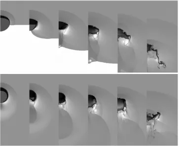
Figure 1. The time evolution of the logarithmic density for models (top)c1shockand (bottom)c1wind1. The grey-scale shows the logarithm of the mass density, from white (lowest density) to black (highest density). The density in this and subsequent figures has been scaled with respect to the ambient density, so that a value of 0 represents the value ofρamband 1 represents 10×ρamb, and the density scale used for this figure extends from 0 to 1.7. The evolution
proceeds left to right witht=0.43tcc,t=0.82tcc,t=1.2tcc,t=1.6tcc,t=2.0tccandt=3.3tcc. Theraxis (plotted horizontally) extends 3rcoff-axis in
each plot. All frames in the top and bottom sets show the same region (−5<z<2, in units ofrc) so that the motion of the cloud is clear. Note that in this and
similar figures thezaxis is plotted vertically, with positive towards the top and negative towards the bottom. Time zero in our calculations is taken to be the time when the
shock is level with the leading edge of the cloud, in the shock-cloud case, whilst for the wind-cloud case the simulation begins with the cloud immediately surrounded by the flow.
3 R E S U LT S
In this section, we present the results from our various simulations. We begin with a brief examination of the interaction of a shock with a cloud in terms of its morphology and then, maintaining the same initial parameters, compare this to the interaction of a wind with a cloud. We then consider in detail the interaction of clouds with winds of increasing Mach number.
At the end of this section, we consider the impact of the interaction on various global quantities. We adopt a naming convention for each simulation such thatc1shockrefers to a shock-cloud simulation with χ=10. Models withwind1a−cin their title indicate wind-cloud interactions of increasing wind Mach number.
3.1 Stages
The purely adiabatic evolution of a cloud struck by a shock propa-gating in the−zdirection is characterized by four main stages (see e.g. Pittard & Parkin2016): (1) the cloud is struck by the shock causing a transmitted shock to travel at a velocityvsthrough the cloud, while a bow shock (or bow wave) is formed upstream and the incident shock diffracts around the cloud; (2) the cloud undergoes compression in thezdirection (on the whole) by both the
transmit-ted shock and also a shock driven into the back of the cloud due to a dramatic pressure jump as the external shock is focused on to the axis; (3) the cloud reaches the expansion stage where, under high pressure, it expands in the radial and axial directions; and (4) the cloud is finally destroyed and mixed with the post-shock flow.
In the case of a wind-swept cloud, stages 1–4 remain essentially the same. However, since the cloud immediately begins interacting with the flow, Banda-Barrag´an et al. (2016) divided the stages for a wind-cloud scenario thus: 1) compression, including the trans-mission and reflection of shocks within, and external to, the cloud; 2) stripping; 3) expansion; and 4) breakup. They noted that the stripping phase (when cloud material begins to flow downstream and wraps around the cloud, converging on the axis behind the cloud) occurs at all times, but is more dynamically important up to
t≈1.3tcc.
3.2 Shock-cloud interaction
We begin by examining the morphology of the interaction for the shock-cloud scenario, where M = 10 and χ = 10 (simulation
c1shock). The shock is initially located atz = 1 (i.e. level with the leading edge of the cloud).
Fig. 1(top panels) provides logarithmic density plots of therz
level with the centre of the cloud att0.32tcc. A bow shock is visible upstream of the cloud. The first three upper panels of Fig. 1
relate approximately to the first two stages of evolution, which lasts untilttcc. The external shock sweeps around the cloud and becomes focused on ther=0 axis. A region of higher pressure forms downstream behind the cloud due to the convergence of this shock on the axis and this serves to drive secondary shocks back through the cloud towards its leading edge. These secondary shocks create additional waves and shocks upstream of the cloud (note the faint secondary shock front just ahead of the cloud in the upper panel att=2.0tccin Fig. 1) when they exit the leading edge of the cloud, accelerating as they do so.
Att1.6tcc the transmitted shock has exited the back of the cloud and accelerates into the downstream gas. This action initiates a rarefaction wave which propagates in the upstream direction. The secondary shocks deposit vorticity as they progress back through the cloud. This deposition begins to disrupt the smooth morphol-ogy of the cloud, forcing the right-hand edge of the cloud upwards and leading to a modest expansion of the cloud in the transverse direction. At the same time, a supersonic vortex ring forms down-stream of the cloud on ther=0 axis. In a similar manner to e.g. Pittard et al. (2009) and Pittard & Parkin (2016), the cloud exhibits a low-density interior surrounded by a thick, high-density shell (see upper panel att=1.6tccin Fig.1). Att2.0tcc, the shell begins to collapse. Cloud material is now ablated by the surrounding flow and shear instabilities at the side of the cloud result in a ‘rolling-up’ of cloud material in the transverse direction – over time this becomes shredded into long strands by the action of KH instabilities on the surface of the cloud. In addition, there is some circulation of the flow on the axis behind the cloud which serves to strip material from the rear of the cloud allowing it to mix in with the flow. After
t3.3tcc, a long, turbulent wake forms on the axis downstream of the cloud and the cloud is quickly ablated.
3.3 Wind-cloud interaction
3.3.1 Comparison of wind-cloud and shock-cloud interactions
Fig. 1(bottom panels) shows logarithmic density plots of therz
plane as a function of time for the wind-cloud case withMwind = 1.36 andχ =10 (simulationc1wind1). The velocity, density and pressure of the wind are exactly the same as the post-shock values in simulationc1shock(i.e. the cloud is surrounded by ‘post-shock’ material). Hence, the density jump between the cloud and the wind is given byχ/3.9 (see Section 2.1).
The morphology of the cloud and its evolution shares some broad similarities with the shock-cloud case (e.g. both clouds form dense shells surrounding lower density interiors, both are squeezed in the radial direction and both are eventually drawn into long, filamentary wakes in the axial direction), but there are also some key differences. First, there are clear differences in the behaviour of the exter-nal medium. Since the simulation begins with the margiexter-nally su-personic wind completely surrounding the cloud, a small lower-density, lower-pressure region is immediately formed on the axis downstream of the cloud (as also noted by Marcolini et al.2005; Banda-Barrag´an et al.2016). This feature is not present in the shock-cloud case and is formed by the initial motion of the wind removing gas from around the rear of the cloud. The low-pressure region is eventually carried downstream of the cloud allowing an area of higher pressure to form behind the cloud (though not in quite the same manner as in thec1shocksimulation).
Secondly, whilst the cloud is strongly compressed into the shape of an oblate spheroid in the shock-cloud case, the cloud in the wind-cloud case suffers much less compression in the axial direction, par-ticularly during the initial stages of the interaction and maintains a more rounded shape. While the leading edge of the cloud undergoes much less compression compared to the shock case, the rear of the cloud is clearly being pushed upwards by the action of a shock driven into the back of the cloud. Plots of the logarithmic pressure (not shown) indicate that a region of high pressure occurs at the lead-ing edge of the cloud in both models, while the back of the cloud remains at a relatively lower pressure in modelc1wind1 compared toc1shock. In their study of a wind-cloud interaction withMwind = 10 (i.e. a higher wind Mach number than used in our model
c1wind1), Schiano, Christiansen & Knerr (1995) noted generally that when a free-flowing wind encounters a 2D spherical cloud and passes through the bow shock, the wind is compressed, decelerated, heated and channelled around the cloud. As the shocked gas is ac-celerated around the periphery of the cloud and rejoins the wind flow along the cloud flanks, the gas pressure is lowered and there is therefore a commensurate decrease in cloud pressure with increas-ing distance from the cloud apex; this is similar to the situation in modelc1wind1.
There are also clear differences between the two simulations in terms of the initial transmitted shock driven through the cloud. In modelc1shock, the shock is reasonably flat as it progresses through the cloud, whereas it is much less flat in modelc1wind1 (cf. both panels att=0.43tccandt=0.82tccin Fig. 1) and curves around the edge of the cloud. As in the shock-cloud case, secondary shocks driven back into the cloud lead to the formation of shocks/waves upstream of the cloud, though in modelc1wind1 these are slightly more pronounced (e.g. att=2.0tcc).
Att=2.8tcc, the cloud, which has developed a dense shell sur-rounding a less dense interior, collapses at a slightly later time than in the shock-cloud case. Eventually, the cloud takes on a very sim-ilar morphology to that in modelc1shockfromt3.3tcconwards, when it is drawn into a long wake in the axial direction (not shown).
3.3.2 Effect of increasing Mwindon the evolution
Fig. 2shows the time evolution of the logarithmic density for modelsc1wind1a,c1wind1b, andc1wind1c, where the wind has an increasing Mach number (Mwind=4.3, 13.6 and 43, respectively). As can be seen from a comparison between Fig. 2and the lower panels of Fig. 1, there are a large number of differences between these simulations andc1wind1 (whereMwind=1.36).
First, as the effective Mach number of the wind increases, the re-gion of low pressure behind the cloud becomes a very low-pressure cavity, is highly supersonic, and expands rapidly in the direction of wind propagation, becoming elongated as it does so. Unlike the initial wind-cloud interaction described above (c1wind1), these cav-ities do not move away from the rear of the cloud and because they are of a much lower pressure than the region inc1wind1 they are far more pronounced.
Secondly, a transmitted shock moves inwards from the back of the cloud inc1wind1 but not in the higherMwind simulations. Whilst the wind flow around the cloud in modelc1wind1 is focused around the cloud flank and on to ther=0 axis, in modelsc1wind1b
2432
K. J. A. Goldsmith and J. M. Pittard
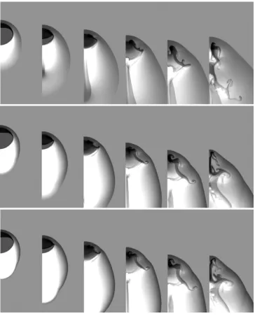
Figure 2. The time evolution of the logarithmic density for models (top)c1wind1a, (middle)c1wind1band (bottom)c1wind1c. The grey-scale shows the logarithm of the mass density scaled with respect to the ambient medium. The density scale used in this figure extends from 0 to 1.7. The evolution proceeds left to right witht=0.7tcc,t=1.3tcc,t=1.9tcc,t=2.6tcc,t=3.2tccandt=5.2tcc. Theraxis (plotted horizontally) extends 3rcoff-axis in each plot. The
first five frames in each set show the same region (−5<z<2, in units ofrc) so that the motion of the cloud is clear. The displayed region is shifted in the last
[image:6.595.43.283.608.682.2]frame in each set (−7<z<0) in order to more fully show the cloud.
Table 2. Values of the density jump and bow shock stand-off distance (in units ofrc) for each of the simulations.
Simulation Density jump Stand-off distance
c1shock 1.53 1.72
c1wind1 1.53 1.72
c1wind1a 3.44 1.32
c1wind1b 3.94 1.28
c1wind1c 3.99 1.28
Thirdly, it is noticeable that the density jump at the bow shock and the stand-off distance between the bow shock and the leading edge of the cloud both change according to the Mach number (see Table 2). As the Mach number of the wind increases, the density
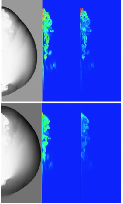
Figure 3. The time evolution of the linear density (left), advected scalar κwhich identifies only the cloud material (middle) and advected scalar ×linear density which allows the density of only the cloud to be shown (right) for modelc1wind1c. The grey-scale shows the mass density, scaled with respect to the ambient medium. The density scale used in the left-hand panels of this figure extends from 0 to 9.7 in the upper panels and 0 to 7.0 in the lower panels. The colour scale in the middle frames extends from dark blue (ambient material) to red (cloud material). The scale used in the right-hand panels extends from 0 to 1 (the ambient medium has a density of 1, but an advected scalar of 0, in this plot). All of the top panels are att=46.0tcc, whilst all the bottom panels are att=101.4tcc. Ther
axis (plotted horizontally in each frame) extends 12rcoff-axis in the top
set of frames and 16rcoff-axis in the bottom set of frames. All frames
in the top set show the same region (−115<z<−85, in units ofrc)
whilst all frames in the bottom set show−250<z<−210.
Although the shape of the cloud in all the wind-cloud simulations with higher values ofMwindis similar, compared to that in model
c1wind1, it is noticeable that the cloud in modelc1wind1abecomes more kinked on its leading edge with the kink resembling the begin-nings of a finger of cloud material moving in the+zdirection, and that the development of this kink is different, compared to models
c1wind1bandc1wind1cwhere the kink is more curled and resem-bles a KH instability (cf. final two panels in each set of Fig. 2). The effect of this kink on the lifetime of the cloud is discussed in Section 3.4.1.
It should be noted that the cloud morphology and statistics in simulationsc1wind1bandc1wind1care very similar (as expected from Mach scaling – cf. Klein et al.1994; Pittard et al.2010).
Fig. 3shows the density, advected scalarκand advected scalar ×density for model c1wind1c at late times (i.e.t = 46tcc and
Table 3. A summary of the cloud-crushing time,tccfor a cloud withχ=10
andrc=1 (see equation 10 for the calculation oftcc), and key time-scales, in
units oftcc, for the simulations investigated in this work. Note that the value
fortdraggiven here is calculated using the definition given in Section 2.3, in
comparison to the values shown in Fig.5which were calculated using the definition given in Pittard et al. (2010) in order to compare with the values oftdragpresented in that paper.
Simulation tcc tdrag tmix tlife
c1shock 0.233 2.35 6.72 23.0
c1wind1 0.233 3.34 6.12 12.9
c1wind1a 0.074 3.88 13.3 35.7
c1wind1b 0.023 3.78 23.5 96.9
c1wind1c 0.0074 4.28 25.6 136.0
t= 101tcc). It can clearly be seen that the cloud has yet to be smoothed out into the flow and shows some evidence of structure along with a distinct cloud edge. Compared with the lower panels in Fig. 2, which show the cloud during the initial stages of the evolution, the cloud in Fig. 3has expanded supersonically into the flow and formed a tail-like structure. Although the cloud is not highly dense at late times, we can infer that it, none the less, shows evidence of long-term survival, something that has not been observed in previous wind-cloud studies.
3.4 Statistics
We now explore the evolution of various global quantities of the interaction for both the shock-cloud and wind-cloud models. Fig. 4
shows the time evolution of these key quantities, whilst Table3lists various time-scales taken from these simulations. The following subsections present a more detailed discussion of these statistics.
3.4.1 Cloud mass
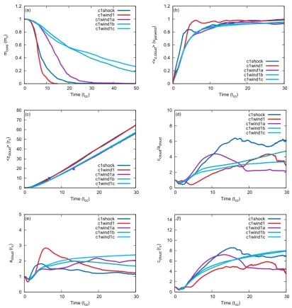
Panel (a) of Fig. 4shows the time evolution of the core mass,mcore. The core mass decreases as a result of cloud material being ablated by, and mixed into, the surrounding flow. It is clear that models
c1shockand c1wind1 share a similar trend in terms of their rate of mass loss, until around two fifths of their core mass has been lost (both models have a much steeper rate of mass loss, at least untilt≈8tcc, than the models with higher values ofMwind). This is surprising considering that the clouds in these simulations ini-tially evolve very differently; for example, the passage of the shock through the cloud, the degree of compression of the cloud and the presence or otherwise of a low-pressure region behind the cloud are different between the two simulations, leading to a difference in cloud morphology. In contrast, modelsc1wind1bandc1wind1c
display very shallow curves which are almost coincident. This re-duced rate of mass loss may be due to the lack of a transmitted shock being driven into the back of the cloud (in contrast to models
c1shockandc1wind1), as well as reduced circulation of the flow on the axis behind the cloud asMwindincreases. In addition, the normal-ized wind velocity (in units ofvwind) is reduced around the cloud flank due to the increased compression at the bow shock. Thus, there is less stripping of material from the rear of the cloud com-pared to lowerMwindsimulations.
[image:7.595.310.549.134.206.2]2434
K. J. A. Goldsmith and J. M. Pittard
Figure 4. Time evolution of (a) the core mass of the cloud,mcore, (b) the mean velocity of the cloud in thezdirection,vz, (c) the centre of mass in the axial direction,zcloud, (d) the ratio of cloud shape in the axial and transverse directions,ccloud/acloud, (e) the effective transverse radius of the cloud,acloudand (f)
the effective axial radius of the cloudccloud. Note that panel (a) shows the evolution on an extended time-scale compared to the other panels. Panel (c) also
shows the position of each cloud att=tmix(indicated by the respective coloured crosses).
simulations c1wind1a − c, a prominent ‘kink’ develops on the leading edge of the cloud; this feature is not evident in Fig. 2of Pittard & Parkin (2016) but the difference may be attributable to the fact that we used a hard edge to our cloud which is more conducive to the growth of such instabilities. A similar kink is present in the adiabatic cloud modelled in Marcolini et al. (2005). This kink allows a greater expansion of the cloud in the radial direction (i.e.
acloud increases) at later times compared to modelsc1shock and
c1wind1. The kink develops differently between modelsc1wind1a
and c1wind1b/c, and the radial expansion of the cloud in model
c1wind1aoccurs earlier than that of the latter two models. This means that the subsequent mixing and ablation of cloud material by the flow takes place earlier than in modelsc1wind1bandc1wind1c. Pittard & Parkin (2016) showed that the mixing time,tmix, for a spherical cloud struck by a Mach 10 shock was≈6tccand increased as the value of the shock Mach number was reduced. Table 3shows
that the two models with similar initial parameters (c1shockand
c1wind1) have roughly similar mixing times. However, forwindsof increasing Mach number the value oftmixincreasesuntil near to the high Mach number limit (whenMps/wind10). As before, this is due to the less effective stripping of cloud material by the flow around the edge of the cloud asMwindincreases. It is surprising, however, to find that the normalized mixing time is five times longer for clouds in winds than for clouds hit by shocks in the high Mach number limit.
3.4.2 Cloud velocity
with the cloud inc1wind1 being accelerated to the velocity of the background flow much more quickly than in the other wind sim-ulations. In addition, in modelc1shock(and to a much lesser ex-tentc1wind1), the cloud exhibits a ‘two-stepped’ acceleration at
t≈4tcc. This coincides with the beginning of a ‘plateau’ region. At this point, the cloud undergoes significant stretching in the axial direction untilt≈8tcc(the approximate end of the plateau region), when most of the core material has been ablated and the remaining less dense and filamentary structure is again accelerated by the flow up to the asymptotic velocity.
The acceleration of the cloud in model c1wind1ais initially smooth untilt≈ 15tcc (at which point the cloud begins to form long strands), but then fluctuates slightly about the velocity of the wind. The clouds in modelsc1wind1bandc1wind1cundergo the smoothest acceleration because of the reduction in the growth of turbulent instabilities on the cloud surface, and again are almost identical in behaviour (due to Mach scaling).
3.4.3 Centre of mass of the cloud
The distance travelled by the cloud before it becomes fully mixed into the flow is reflected by the movement of the cloud centre of mass. The time evolution of the position of the centre of mass of the cloud in thezdirection, normalized by the initial radius of the cloud, is given in Fig. 4(c). It is clear that the post-shock flow or wind can transport cloud material over large distances. Up untilt≈2tcc, there is not a great deal of movement in the direction of the flow (the centre of mass has only moved 0.8−1.8rc). However, byt=12tcc the clouds have been displaced by 15−20 times the initial cloud radius. Over much longer time spans [e.g. up tot=30tcc, as in Fig. 4(c)], the cloud displacement shows greater variation between models, with the centre of mass of the cloud in modelsc1shockand
c1wind1 showing considerably more movement. However, there is much less variety in displacement among all the higher wind Mach number simulations, indicating that movement in the axial direction is not strongly dependent uponMwind in these cases (as expected with Mach scaling). Fig. 4(c) also shows the displacement of each cloud att=tmix. Clearly, the distance over which the cloud has moved by the time its core mass has been reduced by half increases dramatically according to the Mach number, with the cloud in model
c1wind1chaving moved by 47rc attmix (compared to 8rcfor the cloud in modelc1wind1). This indicates that clouds in higher Mach number winds can travel significant distances before being fully mixed into the flow.
3.4.4 Cloud shape
Figs4(d)–(f) show the time evolution of the effective cloud radii,
aandc, and their ratio. The radial dimension of the cloud,acloud, decreases slightly during the initial compression phase as the cloud is squeezed in the axial direction, but then increases sharply as the cloud undergoes expansion. Modelc1wind1 shows the steepest increase, reaching a maximum value foracloud of≈2.8rc att= 5.9tcc as the cloud material is squeezed in the radial direction by the various shocks within and around the cloud, and then decreasing gently as the cloud material is drawn along the axis behind the cloud and gradually mixed into the flow. Modelc1shockfollows a similar trend, though it reaches its peak expansion of 1.8 rcat a slightly earlier time (t=4.4tcc).
The clouds in modelsc1wind1bandc1wind1cshow completely different behaviour, with a more smoothly increasing expansion
over time asMwindincreases, rather than an initial peak. The cloud in modelc1wind1a, as noted earlier, displays traits of both behaviours since it shows a slight initial increase before plateauing and then gently increasing again, eventually peaking at an effective radius of 2.2rcatt=19.5tcc.
Since the cloud in simulationc1shockrapidly becomes elongated in the axial direction after the initial compression of the cloud, the values ofccloud andccloud/acloudsteadily increase over time untilt ≈17tccwhen they level out. The cloud in simulationc1wind1, in contrast, shows a much less steep increase inccloudandccloud/acloud. However, the ratio of cloud shape,ccloud/acloud, shows a much higher value for the cloud in modelc1wind1, reaching a value of 26 at
t=97tcc(not shown) while that for modelc1shockreaches a high of 8.5 att=55tcc. This is in line with Klein et al. (1994), who noted that the combined effect of the lateral expansion associated with the Venturi effect and the axial stretching due to the stripping of material from the side of the cloud led to a much larger cloud aspect ratio for a wind-swept cloud, in comparison to the case of a cloud struck by a shock.
Similar to the above, modelsc1wind1band c1wind1cshow a steady increase in bothccloudandccloud/acloud(with the plots having very similar profiles for both clouds). In contrast to modelc1wind1, the clouds in these two simulations have maximum aspect ratios of 11.3 (att=221tcc) and 4.4 (t=214tcc) (not shown), respectively, which do not follow the behaviour predicted by Klein et al. (1994). The cloud in modelc1wind1ashows different behaviour, again, with an initial peak aroundt≈10−12tccfor bothccloudandccloud/acloud before levelling off. The peak value for the aspect ratio is 16 at
t=79tcc.
3.4.5 Time-scales
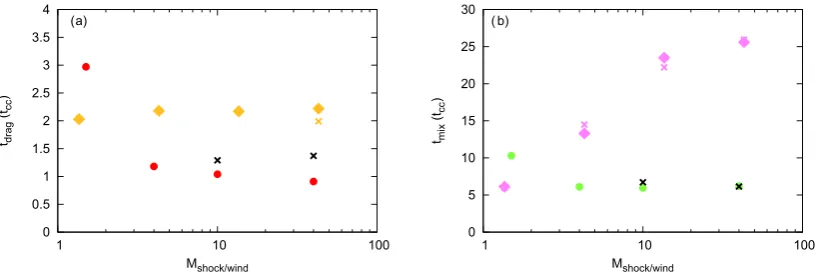
Fig. 5shows the Mach dependence of tdrag andtmix. These two time-scales are useful indicators of the evolution and destruction of the cloud. In previous shock-cloud studies (e.g. Pittard et al.2010; Pittard & Parkin2016), values oftdragandtmixfor a givenχ were relatively constant at Mach numbers> 4 (due to Mach scaling), while at lower Mach numberstdragandtmixboth increased sharply. With the wind-cloud simulations, however, we see that the values for
tmixincrease sharply and nearly linearly (at least forMwind<10) as the Mach number increases. The values fortdragfor the wind-cloud simulations, meanwhile, are relatively constant within the range 2.0 −2.2tcc(using the definition oftdragfound in Pittard et al.2010).3 Within this range the cloud in modelc1wind1 has the lowest value fortdrag, indicating faster acceleration, and that in modelc1wind1c has the highest value (slower acceleration), which fits in with the results of Scannapieco & Br¨uggen (2015) who showed that the acceleration of clouds in galaxy outflows was smaller for higher Mach numbers. While the lack of a shock driven into the back of the cloud in the higher wind Mach number simulations would aid the acceleration of the cloud, it is probable that this effect
3The calculations performed in Pittard et al. (2010, against which we
2436
K. J. A. Goldsmith and J. M. Pittard
Figure 5. (a) Cloud drag time,tdrag, (gold diamonds) and (b) mixing time of the core,tmix, (pink diamonds) as a function of the wind Mach number for
the wind-cloud simulations. The time-scales for all wind-cloud simulations in this paper which were re-run using thek-turbulence model are also shown (gold and pink crosses for panels (a) and (b), respectively. Note that these simulations were run at a slightly lower resolution ofR64). Also shown are the
corresponding values as a function of the shock Mach number for shock-cloud simulations withMshock=10 andMshock=40 (black crosses in each panel), as
well as values from the 2Dk-simulations in Pittard et al. (2010) for a shock-cloud interaction withχ=10 (tdrag, red circles;tmix, green circles). It should
be noted, however, that Pittard et al. (2010) used a slightly different definition of the drag time – defined in their paper as the time when the relative cloud velocity had decreased by a factor of 1/e. This definition provides smaller values oftdragthan the calculation used in this paper. In order to compare the two
time-scales, we re-calculated our values oftdragfor both the shock-cloud simulations where the shock Mach numberM=10 andM=40 and the wind-cloud
simulations in accordance with their definition. See Table 3for values oftdragcalculated according to the definition given in Section 2.3 of the current paper.
is superseded by the reduction in the stand-off distance leading to greater compression at the bow shock and a reduction in the normalized wind velocity around the edge of the cloud.
Figs 4(a) and 5(b) show that the mixing of the core is more efficient atlowerwind Mach numbers. At lowerMwind, the growth of KH instabilities is more important and the post-bow shock velocity of the wind around the cloud flanks is greater. At higherMwind,tmix levels off at25tcc, indicating that Mach scaling is obtained.
Fig. 5shows that the ‘inviscid’ and ‘k-’ models generally have
comparabletdragandtmixtime-scales, indicating that the level of ‘am-bient’ turbulence in the latter has little effect on the cloud evolution (higher values are required – see Pittard et al.2009and Goodson et al.2017). Instead, one sees much larger differences intdrag and
tmixbetween the shock-cloud and wind-cloud cases, indicating that thenatureof the background flow is important.
4 D I S C U S S I O N
The interaction of both shocks and winds with clouds is of great importance in terms of understanding the nature and evolution of the ISM. Shock-cloud and wind-cloud interactions have been studied numerically but there has been no direct comparison of the two processes, to date. In the following subsections, we discuss two main outcomes of our work, Mach scaling and the long-term survival of the cloud. These have previously been discussed in terms of shock-cloud interactions and we note their importance to wind-cloud studies.
4.1 Mach scaling
One of the main results from this study is the presence of Mach scal-ing. Mach scaling has been discussed in detail in previous shock-cloud studies (see e.g. Klein et al.1994; Pittard et al.2009,2010). Briefly, in the strong shock limit, the time evolution of the cloud is independent of the shock Mach number when it is expressed in units oft/tcc∝tMin the limit M→ ∞. Klein et al. (1994) first demonstrated Mach scaling for sharp-edged clouds, with Naka-mura et al. (2006) producing similar results for clouds with smooth
edges. Such studies have been able to demonstrate Mach scaling in the shock-cloud case because the shock Mach numbers used in individual studies have encompassed a large range (e.g. Klein et al.
1994who investigatedM=10−103and Nakamura et al.2006 who used the rangeM=1.5−103). The same cannot be said for wind-cloud studies. A brief trawl of the literature reveals only a handful of studies where the Mach number of the wind was higher than 10. Poludnenko, Frank & Mitran (2004) in their study of hyper-sonic radiative bullets, stated that they had used Mach numbers in the range 10–200 but did not go on to discuss the effect of changing the Mach number on the interaction. Raga et al. (2007), who had very similar parameters to those used in the previous study, used a bullet Mach number of 242 which, whilst firmly in the strong shock regime, was not compared to other values of the Mach number. Pittard et al. (2005) considered wind Mach numbers of 1 and 20 in their study of multiple clouds embedded in a wind, but did not have a great enough range of values for the Mach number in order to detect Mach scaling.
Although there are differences in the initial set-up and the physi-cal processes included, our work is perhaps most easily compared to that of Scannapieco & Br¨uggen (2015), who investigated a range of wind Mach numbers (from 0.5 to 11.4). A key result from these au-thors was that the mixing time-scale increases with the wind Mach number. However, by extending our investigation to higher wind Mach numbers (Mwind = 43.0 versus 11.4) we are able to show that the mixing time levels off at high Mach numbers. We believe therefore that our paper is the first to demonstrate Mach scaling in a wind-cloud study.
4.2 Longer survivability of clouds
In their study, Scannapieco & Br¨uggen (2015) note that clouds embedded in a wind are unable to travel distances of more than 30 −40rcbefore being disrupted. We find that clouds can travel 40− 50rcbyt=tmix, which suggests similarities between our works.
distances over which the clouds were able to travel would enable them to arrive at a few kpc from the driving region; observations have shown these to be typical distances when clouds are seen in absorption against the starbursting host galaxy (see e.g. Heckman et al.2000; Pettini et al.2001; Soto & Martin2012). These clouds would therefore require a distinct density (as opposed to the cloud mass being smoothed out and mixed into the flow) in order to be ob-served in this way. Absorption line observations using background galaxies and quasars have in fact revealed that clouds may travel dis-tances on the order of≈100 kpc or more (Bergeron1986; Lanzetta & Bowen1992; Steidel, Dickinson & Persson1994; Steidel et al.
2002,2010; Zibetti et al.2007; Kacprzak et al.2008; Chen et al.
2010; Tumlinson et al.2013; Werk et al.2013,2014; Peeples et al.
2014; Turner et al.2014). This is extremely challenging for current theoretical models.
In our study, we find that the cloud in simulationc1wind1c, i.e. the simulation with the highest wind velocity and a cloud den-sity contrast of 10, still has significant structure and denden-sity at late times (e.g. 100tcc, when it still has≈10 per cent of its core mass; see Fig. 3) and that it is able to reach distances of 200rc at this time (see Fig. 3). Thus, although our results are still not eas-ily reconciled with observations indicating clouds existing at the 100 kpc distances noted above, they none the less show that clouds can survive as distinct structures over much longer distances com-pared to those presented in Scannapieco & Br¨uggen (2015). The longer survivability of clouds entrained in a wind may be further en-hanced when combined with other effects such as magnetic fields or cooling.
Fig. 3shows that the cloud in simulationc1wind1cis not com-pletely destroyed at late times, though its density has dropped below that of the surrounding wind byt≈100tcc(the bottom panels of Fig. 3). Since the bow shock around the cloud is denser than the cloud at this time, preferential detection of the cloud may require that the cloud material has enhanced metallicity relative to the wind (cf. Turner et al.2014).
5 S U M M A RY A N D C O N C L U S I O N S
In this paper, we compared the interaction between a shock and a spherical cloud with that of a wind-cloud interaction with similar initial parameters. Our motivation was the lack of any paper in the literature that directly compared these two processes and the general supposition that shock-cloud and wind-cloud interactions were broadly comparable. However, we found there to be subtle, but also significant, differences between the two types of interaction.
We first compared our wind-cloud simulations against a shock-cloud simulation withM=10 andχ=10 (c1shock). Our standard wind-cloud simulation (c1wind1) has the same cloud completely embedded in a (slightly supersonic) wind with exactly the same properties as the post-shock flow in modelc1shock. We find that the subsequent behaviour of the external medium differs between the two cases. In the particular case of a marginally supersonic wind, an area of low pressure immediately forms downstream behind the cloud (a feature not present in the shock-cloud case). There are also differences in the morphology of the cloud itself. A cloud en-gulfed by a marginally supersonic wind undergoes less compression than that struck by a shock because the flow around the cloud is diffracted in a different way to the shock-cloud case. Finally, there are noticeable differences in the initial transmitted shock between the shock-cloud and wind-cloud simulations; the shock in the for-mer is far flatter in shape whereas that in modelc1wind1 curves around the edge of the cloud.
As the effective Mach number of the wind increases, the mor-phological differences between the wind simulations and the shock simulation become more prominent. The cavitation behind the cloud becomes more supersonic and highly elongated. The higher Mach number causes a greater density and pressure jump behind the bow shock, leading to reduced normalized post-bow shock gas veloci-ties around the cloud flank. Because of this, KH instabiliveloci-ties become slightly weaker asMwindincreases. Another difference is that clouds in simulations with a high wind Mach number do not experience the formation of transmitted shocks on the axis behind the cloud. In addition to the morphological changes, we also showed that the mixing time increases for increasingMwind, which is in contrast to the findings of Pittard & Parkin (2016) with respect to a shock-cloud interaction. Our simulations also display Mach scaling in the high Mach number limit. The density jump at the bow shock asymptotes to 4.0 (forγ =5/3), and the stand-off distance between the bow shock and the centre of the cloud asymptotes to 1.28rc(again for γ =5/3). The morphology of the cloud and the normalized ac-celeration and mixing time-scales plateau at high Mach numbers. Moreover, we found that clouds embedded in winds with highMwind survived for longer, and travelled over larger distances, compared to the results of the wind-cloud study by Scannapieco & Br¨uggen (2015).
The models used in this work have several limitations. First, this was a 2D study with imposed axisymmetry. Secondly, we consid-ered only spherical clouds with sharp edges (i.e. our clouds had no distinct core and surrounding envelope but were uniformly dense) and neglected physical processes such as radiative cooling and mag-netic fields. Therefore, future comparisons should consider more realistic cloud models and scenarios reflecting a more complex, in-homogeneous ISM/intergalactic medium. However since our work is scale-free, our results can be applied to a broad range of problems related to the gas dynamics of the ISM. A follow-up paper to the present study will compare shock-cloud and wind-cloud interac-tions where the cloud density contrast is higher.
AC K N OW L E D G E M E N T S
We would like to thank the referee, Alejandro Raga, for construc-tive comments that helped to clarify and generally improve the manuscript. This work was supported by the Science & Tech-nology Facilities Council [Research Grants ST/L000628/1 and ST/M503599/1]. We thank S. Falle for the use of theMG hydro-dynamics code used to calculate the simulations in this work. The calculations used in this paper were performed on the DiRAC Fa-cility which is jointly funded by STFC, the Large Facilities Capital Fund of BIS and the University of Leeds. The data associated with this paper are openly available from the University of Leeds data repository.http://doi.org/10.5518/120.
R E F E R E N C E S
Al¯uzas R., Pittard J. M., Hartquist T. W., Falle S. A. E. G., Langton R., 2012, MNRAS, 425, 2212
Al¯uzas R., Pittard J. M., Falle S. A. E. G., Hartquist T. W., 2014, MNRAS, 444, 971
Banda-Barrag´an W. E., Parkin E. R., Crocker R. M., Federrath C., Bicknell G. V., 2016, MNRAS, 455, 1309
Bergeron J., 1986, A&A, 155, L8
Bruhweiler F. C., Ferrero R. F., Bourdin M. O., Gull T. R., 2010, ApJ, 719, 1872
2438
K. J. A. Goldsmith and J. M. Pittard
Cooper J. L., Bicknell G. V., Sutherland R. S., Bland-Hawthorn J., 2008, ApJ, 674, 157
Cooper J. L., Bicknell G. V., Sutherland R. S., Bland-Hawthorn J., 2009, ApJ, 703, 330
Cowie L. L., McKee C. F., Ostriker J. P., 1981, ApJ, 247, 908 Dyson J. E., Arthur S. J., Hartquist T. W., 2002, A&A, 390, 1063 Elmegreen B. G., Scalo J., 2004, ARA&A, 42, 211
Falle S. A. E. G., 1991, MNRAS, 250, 581 Farris M. H., Russell C. T., 1994, JGR, 99, 17681
Fragile P. C., Murray S. D., Anninos P., van Breugel W., 2004, ApJ, 604, 74 Goldsmith K. J. A., Pittard J. M., 2016, MNRAS, 461, 578
Goodson M. D., Heitsch D., Eklund K., Williams V. A., 2017, MNRAS, 468, 318
Gregori G., Miniati F., Ryu D., Jones T. W., 1999, ApJ, 527, L113 Gregori G., Miniati F., Ryu D., Jones T. W., 2000, ApJ, 543, 775 Hansen J. F., Robey H. F., Klein R. I., Miles A. R., 2007, ApJ, 662, 379 Heckman T., Lehnert M. D., Strickland D. K., Lee A., 2000, ApJS, 129, 493 Hennebelle P., Falgarone E., 2012, A&AR, 20, 55
Johansson E. P. G., Ziegler U., 2013, ApJ, 766, 45 Jones T. W., Ryu D., Tregillis I. L., 1996, ApJ, 473, 365
Kacprzak G. G., Churchill C. W., Steidel C. C., Murphy M. T., 2008, AJ, 135, 922
Klein R. I., McKee C. F., Colella P., 1994, ApJ, 420, 213
Klein R. I., Bundil K. S., Perry T. S., Bach D. R., 2003, ApJ, 583, 245 Koo B-C., Rho J., Reach W. T., Jung J., Mangum J. G., 2001, ApJ, 552, 175 Lanzetta K. M., Bowen D. V., 1992, ApJ, 391, 48
Li S., Frank A., Blackman E. G., 2013, ApJ, 774, 133 Mac Low M.-M., Klessen R., 2004, Rev. Mod. Phys., 76, 125
Mac Low M.-M., McKee C. F., Klein R. I., Stone J. M., Norman M. L., 1994, ApJ, 433, 757
Marcolini A., Strickland D. K., D’Ercole A., Heckman T. M., Hoopes C. G., 2005, MNRAS, 362, 626
Martin C. L., 2005, ApJ, 621, 227
Martin C. L., Shapley A. E., Coil A. L., Kornei K. A., Bundy K., Weiner B. J., Noeske K. G., Schiminovich D., 2012, ApJ, 760, 127
McCourt M., O’Leary R. M., Madigan A. -M., Quataert E., 2015, MNRAS, 449, 2
McKee C. F., Ostriker J. P., 1977, ApJ, 218, 148 McKee C. F., Ostriker E. C., 2007, ARA&A, 45, 565
Mellema G., Kurk J. D., R¨ottgering H. J. A., 2002, A&A, 395, L13 Nakamura F., McKee C. F., Klein R. I., Fisher R. T., 2006, ApJ, 164, 477 Orlando S., Peres G., Reale F., Bocchino F., Rosner R., Plewa T., Siegel A.,
2005, A&A, 444, 505
Orlando S., Bocchino F., Reale F., Peres G., Pagano P., 2008, ApJ, 678, 274 Padoan P., Federrath C., Chabrier G., Evans N. J., II, Johnstone D., Jørgensen J. K., McKee C. F., Nordlund ˙A., 2014, in Beuther H., Klessen R. S., Dullemond C. P., Henning T., eds, Protostars and Planets VI. University of Arizona Press, Tucson, p. 77
Peeples M. S., Werk J. K., Tumlinson J., Oppenheimer B. D., Prochaska J. X., Katz N., Weinberg D. H., 2014, ApJ, 786, 54
Peretto N. et al., 2012, A&A, 541, A63
Pettini M., Shapley A. E., Steidel C. C., Cuby J.-G., Dickinson M., Moorwood A. F. M., Adelberger K. L., Giavalisco M., 2001, ApJ, 554, 981
Pittard J. M., Goldsmith K. J. A., 2016, MNRAS, 458, 1139 Pittard J. M., Parkin E. R., 2016, MNRAS, 457, 4470
Pittard J. M., Arthur S. J., Dyson J. E., Falle S. A. E. G., Hartquist T. W., Knight M. I., Pexton M., 2003, A&A, 401, 1027
Pittard J. M., Dyson J. E., Falle S. A. E. G., Hartquist T. W., 2005, MNRAS, 361, 1077
Pittard J. M., Falle S. A. E. G., Hartquist T. W., Dyson J. E., 2009, MNRAS, 394, 1351
Pittard J. M., Hartquist T. W., Falle S. A. E. G., 2010, MNRAS, 405, 821 Poludnenko A. Y., Frank A., Blackman E. G., 2002, ApJ, 576, 832 Poludnenko A. Y., Frank A., Mitran S., 2004, ApJ, 613, 387
Raga A., Steffen W., Gonz´alez R., 2005, Rev. Mex. Astron. Astrofis., 41, 45 Raga A. C., Esquivel A., Riera A., Vel´azquez P. F., 2007, ApJ, 668, 310 Rogers H., Pittard J. M., 2013, MNRAS, 431, 1337
Rupke D. S., Veilleux S., Sanders D. B., 2002, ApJ, 570, 588
Sales L. V., Navarro J. F., Schaye J., Dalla Vecchia C., Springel V., Booth C. M., 2010, MNRAS, 409, 1541
Scalo J., Elmegreen B. G., 2004, ARA&A, 42, 275 Scannapieco E., Br¨uggen M., 2015, ApJ, 805, 158
Schiano V. R., Christiansen W. A., Knerr J. M., 1995, ApJ, 439, 237 Schneider N., Bontemps S., Simon R., Jakob H., Motte F., Miller M., Kramer
C., Stutzki J., 2006, A&A, 458, 855
Shin M.-S., Stone J. M., Snyder G. F., 2008, ApJ, 680, 336 Soto K. T., Martin C. L., 2012, ApJ, 203, 3
Steidel C. C., Dickinson M., Persson S. E., 1994, ApJ, 437, L75
Steidel C. C., Kollmeier J. A., Shapley A. E., Churchill C. W., Dickinson M., Pettini M., 2002, ApJ, 570, 526
Steidel C. C., Erb D. K., Shapley A. E., Pettini M., Reddy N., Bogosavljevi´c M., Rudie Gwen C., Rakic O., 2010, ApJ, 717, 289
Tumlinson J. et al., 2013, ApJ, 777, 59
Turner M. L., Schaye J., Steidel C. C., Rudie G. C., Strom A. L., 2014, MNRAS, 445, 794
Wareing C., Pittard J. M., Falle S. A. E. G., 2017, MNRAS, 465, 2757 Werk J. K., Prochaska J. X., Thom C., Tumlinson J., Tripp T. M., O’Meara
J. M., Peeples M. S., 2013, ApJS, 204, 17 Werk J. K. et al., 2014, ApJ, 792, 8
Westmoquette M. S., Slavin J. D., Smith L. J., Gallagher J. S., 2010, MNRAS, 402, 152
White R. L., Long K. S., 1991, ApJ, 373, 543 Xu J., Stone J. M., 1995, ApJ, 454, 172
Yirak K., Frank A., Cunningham A. J., 2010, ApJ, 722, 412
Zibetti S., M´enard B., Nestor D. B., Quider A. M., Rao S. M., Turnshek D. A., 2007, ApJ, 658, 161