A multiscale method for optimising surface topography in elastohydrodynamic lubrication (EHL) using metamodels

RESEARCH PAPER

A multiscale method for optimising surface topography

in elastohydrodynamic lubrication (EHL) using metamodels

G. N. de Boer1&L. Gao1&R. W. Hewson1&H. M. Thompson2&

N. Raske3&V. V. Toropov3

Received: 1 October 2015 / Revised: 11 December 2015 / Accepted: 22 December 2015 / Published online: 2 April 2016 #The Author(s) 2016. This article is published with open access at Springerlink.com

Abstract The frictional performance of a bearing is of significant interest in any mechanical system where there are lubricated surfaces under load and in relative motion. Surface topography plays a major role in deter-mining the coefficient of friction for the bearing because the size of the fluid film and topography are of a com-parable order. The problem of optimising topography for such a system is complicated by the separation in scales between the size of the lubricated domain and that of the topography, which is of at least one order of mag-nitude or more smaller. This paper introduces a multiscale method for optimising the small scale topog-raphy for improved frictional performance of the large s c a l e b e a r i n g . T h e a p p r o a c h f u l l y c o u p l e s t h e elastohydrodynamic lubrication at both scales between pressure generated in the lubricant and deformation of the bounding surfaces. Homogenised small scale data is used to inform the large scale model and is represented using Moving Least Squares metamodels calibrated by cross validation. An optimal topography for a minimum coefficient of friction for the bearing is identified and comparisons made of local minima in the response,

where very different topographies with similar frictional performance are observed. Comparisons of the optimal topography with the smooth surface model demonstrated the complexity of capturing the non-linear effect of to-pography and the necessity of the multiscale method in capturing this. Deviations from the smooth surface mod-el were quantified by the metamodmod-el coefficients and showed how topographies with a similar frictional per-formance have very different characteristics.

Keywords Multiscale method . Bracketing optimisation . Surface topography . Metamodelling . Moving Least Squares . Cross Validation

Abbreviations

BVP Boundary Value Problem

CFD Computational Fluid Dynamics

CV Cross Validation

DOE Design of Experiments

EHL Elastohydrodynamic Lubrication

FSI Fluid structure Interaction

GA Genetic Algorithm

HMM Heterogeneous Multiscale Methods

IVP Initial Value Problem

k-CV k-fold Cross Validation

LOO-CV Leave-One-Out Cross Validation

MLS Moving Least Squares

OLHC Optimum Latin Hypercube

PTFE Polytetrafluoroethlyene

RMSE Root Mean Squared Error

Nomenclature

A MLS matrix

b Right-hand-side variable in the MLS

operation

* G. N. de Boer

[email protected]

1

Department of Aeronautics, Imperial College London, London SW7 2AZ, UK

2

School of Mechanical Engineering, University of Leeds, Leeds LS2 9JT, UK

3 _{School of Engineering and Materials Science, Queen Mary} University of London, London E1 4NS, UK

C1–8 MLS coefficients

E Young’s modulus

E’ Equivalent Young’s modulus

h Undeformed film thickness

g Film gap

G Normalised film gap

I Identity matrix

k Fold size

k1 Local stiffness

K Stiffness matrix

L Cell length

Lp Pad length

N Size of DOE

p Pressure

p* Load per unit area

ps Small scale pressure

P Normalised pressure

dp

dx Pressure gradient

Δp Pressure jump

q Mass flow rate per unit depth

Q Normalised mass flow rate per unit depth

r Normalised Euclidean distance

s Small scale film thickness

Δs Deformation of the small scale film thickness

t Pad thickness

t’ Equivalent thickness

usvs, ws, Small scale velocity components

U Moving wall velocity

w Moving least squares weight

W Load capacity

Wrep Required load capacity

x Large scale coordinate direction

xs, ys, zs, Small scale coordinate directions

α Topography amplitude

γ Left-hand-side variable in the MLS

operation

Γ Vector of MLS multipliers

δ Deformation

δt Topography

η0 Ambient viscosity

ηs Small scale viscosity

θ Closeness of fit parameter

μ Coefficient of friction

ν Poisson’s ratio

ρ0 Ambient density

ρs Small scale density

τ Shear stress

φ Tilt angle

ψ Small scale topography parameter

a Inlet

b Outlet

~

Assessment location

1 Introduction

Elastohydrodynamic Lubrication (EHL) describes the forma-tion of a lubricated film between two machine elements which are under load and in relative motion to each other. The pressurisation of the lubricant in the EHL regime is large enough to cause deformation of the mating surfaces, which in turn leads to a change in the lubricating film thickness. Fluid film lubrication is conventionally modelled using the Reynolds equation (Cameron1971) based on the lubrication between two nearly parallel smooth surfaces. EHL exists in mechanical systems such as gear teeth, bearings, rubber seals and car tyres on a wet road (Dowson1999). One of the design challenges for such systems is to control the coefficient of friction between the mating surfaces, typically to reduce it for machine components and increase it where traction is re-quired. Tzeng and Saibel (1967), Patir and Cheng (1978), Etsion (2005), de Kraker et al. (2007), Sahlin et al. (2010), de Boer et al. (2014) have found that texturing bearing sur-faces can have a significant effect on the coefficient of friction of lubricated contacts compared to the smooth bearing case. Despite the significant work showing potential performance improvements in terms of friction there is still a need for an efficient computational approach to analyse bearing topogra-phy and more importantly to use such analysis for design optimisation.

Minimising friction in a textured EHL contact is compli-cated by the fact that it is a multi-scale problem where the scale of the overall lubricated domain is typically an order of magnitude or more greater than that of the topographical fea-tures (Gohar 2001). This disparity of scales means that it is infeasible to computationally resolve the small scale features as well as the large scale bearing domain. This is especially true when (i) the assumptions on which the Reynolds equation is based (Cameron1971) break down due to the local topog-raphy and the bearing surfaces no longer being nearly parallel, (ii) the deformation of the bearing geometry under the influ-ence of pressurised lubricant is also considered as is the case in EHL.

Kraker et al.2007) and Navier–Stokes flow models (de Boer et al.2014; Gao et al.2015). A similar mulitscale approach has also been used to model coating flows where topograph-ical features are present (Hewson et al.2011).

Data communication between the length-scales of a multi-scale method can be achieved in several ways. Serial coupling methods pass parameters between the scales and determine the effective macroscopic parame-ters from the micro-scale model in a pre-processing step and use the macroscopic model in the computations, see de Kraker et al. (2007) in the context of EHL model-ling. In concurrent coupling methods, however, the micro-scale and macro-scale models are linked dynami-cally during the overall computation (Abraham et al.

1999) and it is therefore important to build a fast input/output relationship between models at the different scales (Roux et al. 1998). The use of metamodels to represent the small-scale data is becoming increasingly

popular. Benke et al. (2009), for example, used

metamodels for the atomic structure of DNA molecules to determine the parameters of the mechanical structures within a multiscale model of polymer migration in DNA-laden flows, and Writz et al. (2015) recently pro-posed the use of kernel methods to provide fast metamodels for multiscale modelling of the human spine. The general metamodelling approach is divided into two stages: a computationally expensive offline stage where the metamodelling parameters are calibrated against a set of training data; and an online computing stage comprising fast execution of the resulting metamodel within the multi-scale modelling framework.

de Boer et al. (2014) used multi-dimensional

metamodels for representing efficiently the small scale model within a macroscopic EHL model. Their metamodel approximations were based on the Moving Least Squares (MLS) method and were calibrated using Cross Validation (CV) techniques combined with effi-cient space-filling Design of Experiments (DOE) (Loweth et al. 2011). The present study will exploit the synergies between multiscale EHL analysis and re-sponse surface enabled optimisation in order to demon-strate a means of achieving multiscale design optimisa-tion across the scales. This will be demonstrated by the optimisation of small scale bearing topography for a minimal coefficient of friction of the bearing system.

The paper is organised as follows. The multiscale EHL method and metamodelling strategies are intro-duced in Section 2. Numerical methods are described in Section 3. In Section 4 the validation and perfor-mance of the metamodel is demonstrated and the opti-mal substrate topography leading, to miniopti-mal frictional drag, identified. Conclusions are drawn in Section 5.

2 Theory

2.1 Problem formulation

The optimisation problem described here represents one fre-quently encountered in the field of tribology, that of how to reduce the coefficient of friction in an EHL contact for a con-stant applied load. The method described is based on the

Heterogeneous Multiscale Methods (E et al. 2007)

whereby homogenised information obtained from periodic small scale models (topography) is used to derive a relation-ship for the large scale model (bearing). An overview of the two-scale method for EHL is given here, a full description can be found in de Boer et al. (2014).

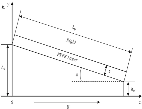
A simple large scale geometry will be considered, that of a 2D linear slider bearing as shown below in Fig.1. The domain between inlet and outlet is fully flooded with lubricant, the lower wall of the bearing moves in the x coordinate direction with velocity U and does not deform, the upper surface is stationary and deformable.

Here the large scale geometry, specifically the pad length Lpand tilt angleφare kept constant, however they could be

varied in order to maximise bearing performance, as would be undertaken for single scale optimisation. To demonstrate the means by which optimisation is undertaken across scales a small scale geometry parameterψis defined. The multiscale optimisation problem is subsequently given by (1)-(3):

min

ψ ð Þμ ð1Þ

0≤ψ≤1 ð2Þ

W hð Þ−b Wreq¼0 ð3Þ

where the objective μ is the bearing coefficient of fric-tion and the constraint W is the bearing load capacity, as calculated by (4) and (5) respectively. Wreq is the

required bearing load which is achieved by varying the minimum undeformed film thickness for the bearing hb

to give the undeformed film thickness h:

μ¼ 1

W Z

0 Lp

τ dp

dx;p;g;ψ

dx ð4Þ

W¼

Z

0 Lp

p* dp dx;p;g;ψ

dx ð5Þ

τ dp dx;p;g;ψ

and p* dp dx;p;g;ψ

To solve the large scale problem and evaluate (i) the load per unit area (which differs slightly from the large scale pres-sure due to the homogenisation approach) and (ii) shear stress, the large scale governing equations for the pressure (6) and lubricant flow rate (7) are solved:

dp dx¼

dp

dxðp;g;q;ψÞ ð6Þ

dq

dx¼0 ð7Þ

The equation for the pressure gradient is also obtained from the small scale simulations, where q is the mass flow rate per unit depth. The large scale solution to (6) and (7) is obtained with Dirichlet boundary conditions for zero (ambient) pres-sure (8) at both inlet and outlet:

p_a¼p_b¼0 ð8Þ

The bearing deformation is accounted for at both the large and small scale in order to account for non-local deformation (deformation at a surface location due to a pressure at a different location on the pad surface) and the micro-elastohydrodynamic surface deformation (de-formation of the small scale domain due to small scale variations in the pressure profile). It is based on the elastic deformation δ which would be encountered in the smooth case and is found via a matrix operation, where the influence of pressure on displacement de-creases with the distance from the point at which it is applied. The total deformation influence matrix K, or deformation coefficient matrix, is calculated using e l a st ic i t y th e o r y b a s ed o n t h e t h ic k n e s s of t h e Polytetrafluoroethylene (PTFE) pad t (Rodkiewicz and Yang 1995). The relationship describing how load per unit area p* relates to deformation is given by δ=Kp*.

This can be rewritten such that total deformation is the sum of two separate terms as given by (9):

δ¼ðK−k1IÞp*þk1Ip* ð9Þ

In (9), k1is the local stiffness which is subsequently

modelled at the small scale, see Section 2.2. The term k1Ip

accounts for local deformation (deformation due to pressure at that location) and (K−k1I)p* the remaining deformations

(de-formation due to pressure at all other locations). The film gap (g) becomes the sum of the undeformed film thickness h and non-local deformation allowing local deformation to be con-sidered at the small scale (including micro-EHL where defor-mation of individual topographical features may occur). (6), (7) and (10) are coupled and solved iteratively until conver-gence in the pressure distribution is reached:

g¼hþðK−k1IÞp* ð10Þ

In defining the optimisation problem the variable defining the small scale geometryψis included in the functional terms defining the pressure gradient dp_dxðp;g;q;ψÞ, shear stress τ

dp dx;p;g;ψ

and load per unit area p* dp dx;p;g;ψ

. This is an important distinction when compared with the analysis case as it means that a representation is required of how the small scale behaves with changes in both the local operating conditions dp_dx;p;g;q as well as the optimisation problem’s design variablesψ (in this case). This representation of the small scale problem is achieved using a metamodel of the small scale behaviour and for this case is therefore 4-dimensional.

2.2 Small scale simulations

A series of small scale simulations were undertaken on which the metamodel was constructed. These small scale simulations were a set of Fluid–Structure Interaction (FSI) problems with the lubricant flow modelled using the Navier–Stokes equa-tions and the local deformation and micro-EHL simulated by an equivalent column of elastic bearing material.

The small scale simulations use an equivalent thickness t′ of the solid domain to ensure that the resulting deformation due to fluid pressure is equal to the column deformation achieved from the local stiffness required k1at the large scale

under the same pressure (11). The equivalent elastic modulus E ' is derived to represent the mechanical properties of the large scale stiffness to a fully constrained column of bearing material in three-dimensions at the small scale (12):

t0¼k1E0 ð11Þ

E0¼ ð1−νÞE 1þν

ð Þð1−2νÞ ð12Þ

where E andνare the Young’s modulus and Poisson’s ratio of the bearing material (PTFE) respectively. By applying an equivalent thickness to the problem the small scale FSI is accurately described whilst maintaining the required stiffness properties at the large scale and of the bearing surface. Structural mechanics at the small scale are considered by im-plementation of a 3D model for a linearly elastic solid, the material is assumed homogenous and isotropic. The upper boundary of the spring column is fully constrained. The sides of the spring column are constrained normal to the surface. The fluid/solid interface is loaded by pressure generated from the fluid flow simulations.

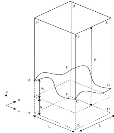
The small scale fluid geometry is defined by a cell length L in both xsand yscoordinate directions, this length scale must

be an order of magnitude or more smaller than the pad length Lp. The zs coordinate is aligned with the film gap g.

Topographyδtis defined by the small scale geometry

param-eterψand the topography amplitudeα(13), this is summed with g to form the small scale film thickness s. The parameter

ψcontrols the ratio of longitudinal to transverse waviness in the topography response, atψ= 0 topography is longitudinal and atψ= 1 topography is transverse to the direction of mo-tion of the bearing surface:

δt¼α

2 ψ sin 2π

xs

L

þ1

h

þð1−ψÞ sin 2πys L

þ1

i ð13Þ

A diagram showing the small scale geometry with both solid and fluid domains is shown in Fig.2.

The small scale flow is modelled using Computational Fluid Dynamics (CFD) where the flow is considered steady, laminar, compressible and isothermal as described by the Navier–Stokes

equations. The lubricant densityρsvaries barotropically as

de-scribed by the Dowson-Higginson equation (Dowson and Higginson 1966). Piezoviscosity is modelled using the Roelands equation (Roelands 1966) and non-Newtonian (shear-thinning) behaviour is considered using the Ree-Eyring model to give the lubricant viscosity ηs (Johnson and

Tevaarwerk1977). The interface between the fluid and solid is a no-slip wall, the lower surface is a moving wall with velocity U, the remaining boundaries are subject to the near-periodic boundary condition. The pressure ps on each set of

near-periodic boundaries experiences a jump Δp over the domain. Velocity components us, vs, wsare scaled at the boundaries to

account for the difference in density (due to pressure at the boundaries) and area (due to deformation of the boundaries).

The generation of the data points from which to generate the response surfaces to be used in the optimisation of the tribology problem requires the homogenisation of the small scale geome-try, it is this homogenisation which leads to the requirement that the small scale domain is at least an order of magnitude smaller than that of the large scale problem, L≪Lp. This is analogous to

the separation of scales between the bearing length and lubricat-ed gap in derivation of the Reynolds equation (the accurate description of smooth surface lubrication) which states that the film thickness varies gradually along the length of the bearing.

Given a pressure constraint, initial gap, and small scale geometry parameter, the solution fields for pressure and ve-locity can be obtained by solving for the small scale model. Coupling of structural mechanics and CFD is achieved through an Arbitrary Lagrangian–Eulerian approach in a Finite Element (FE) simulation. The homogenised pressure gradientdp_dx over a unit cell is calculated using (14), and the mass flow rate per unit depth q is determined from (15) on the periodic boundary normal to the sliding direction:

dp dx¼

Δp

L ð14Þ

q¼ 1 L

Z

0

sþΔsZ L

0

ρsusdysdzs ð15Þ

Pressure is not uniformly distributed in the small scale do-main and so an average cell pressure p* is derived which describes the load per unit area and from which deformation

δand load capacity W are determined at the large scale (16). A similar expression exists for the shear stressτfrom which the coefficient of frictionμis found (17). Both (16) and (17) are calculated on the sliding wall boundary:

p*¼ 1 L2

Z L

0

Z L

0

psdxsdys ð16Þ

τ¼ 1

L2

Z L

0

Z L

0 ηs

dus

dzs

dxsdys ð17Þ

whereΔs is the deformation of the small scale film thickness. A

B

C

D E F

G

H P

Q R

S

g

t'

L L

y x z

2.3 Metamodel construction

The construction of an accurate metamodel representing the terms_dxdpðp;g;q;ψÞ;τdp_dx;p;g;ψand p* dp

dx;p;g;ψ

is crit-ical to both the accurate analysis of the bearing performance and to permit the optimisation of the system. The first stage in constructing the metamodel is the generation of the simulation conditions (both design and operating variables). Creating a model of this nature requires a DOE which ensures the most efficient spread of simulations in the design space, as to reduce the number of simulations while allowing the response to be accurately described. An Optimal Latin Hypercube (OLHC) is used here to explore as much of the design space with as few designs as possible. This is generated using a permutation Genetic Algorithm (GA) to optimise the distance between all DOE points (Bates et al. 2004). This satisfies the Audze-Eglais condition (Audze and Audze-Eglais1977) which requires that the sum of the reciprocal of the squared distances between each DOE point and all others is a minimum.

MLS is derived from conventional weighted least squares model building where the weights do not remain constant but are functions of the normalised Euclidian distances from sam-ple points to the point where the metamodel is evaluated (Choi et al.2001). Coefficients in the basis function of the MLS approximation become functions of the design space and therefore describe how the metamodel varies from the least squares approximation (Breitkopf et al.2005).

Reynolds equation (Cameron1971) is used as the MLS basis function (18), when the coefficients C1−3are unity the

metamodel produces the result obtained directly from smooth surface lubrication (i.e. the pressure gradient Eq. (6) without topography and fluid flow phenomena). Expressions for the load per unit area (19) and shear stress (20) under smooth conditions are also obtained when C4−8are unity. The MLS

coefficients C1−8therefore quantify the deviation from the

smooth surface model when surface topography is included and are functions of the design space considered. In (18)-(20),

ρ0andη0are the ambient density and viscosity of the lubricant

respectively:

dp dx¼

12η0 ρ0ðgþk1pÞ3

C1ρ0U

2 ðgþk1pÞ−C2q

þC3−1 ð18Þ

p*¼C4pþC5−1 ð19Þ

τ¼ 1

gþk1p

C6Uη0þ

C7

2 ðgþk1pÞ

2dp

dx

þC8−1

ð20Þ

A Gaussian decay function is defined for the MLS weights such that the influence of a known sample location will di-minish exponentially with increasing distance to an assess-ment location, as is common in metamodel analyses (de

Boer et al.2014; Loweth et al.2011). Polynomial type decay functions can also be used to formulate the weights (Toropov et al.2005). (26) describes how the weights corresponding to each know location wiare functions of the closeness of fit

parameterθand the normalised Euclidian distance to the as-sessment location ri:

wi¼exp −θr2i

i¼1;…;N ð21Þ

where N is the total number of points in the sample set (DOE size) and riis obtained from (22), in which capitals represented

the normalised version of the corresponding lower case vari-ables and tilde the assessment location of the metamodel:

r2_i ¼ P~−Pi

2

þ G~−Gi

2

þ Q~−Qi

2

þ ψ~−ψi

2 ð22Þ

By minimising the sum of squared error in the MLS ap-proximation and known location values the coefficients in (18) can be determined at the assessment location by the ma-trix Eq. (23). Equation (23) is formulated by the series of Eqs. (24)-(27):

Aγ−b

k k ¼0 ð23Þ

bi¼wi

dp dx _iþ1

ð24Þ

Ai j¼wiΓi j ð25Þ

Γi¼

6Uη₀ g_iþk1pi

ð Þ2

−12η₀q_i

ρ0ðgiþk1piÞ 3 1

ð26Þ

γj¼Cj j¼1;…;3 ð27Þ

Once the coefficients are calculated from (23) the MLS approximation can be determined by (18), substituting the coefficients and determining the polynomial expression for the assessment location. The same approach can be taken to assess the coefficients in (19) and (20).

The MLS approximation can be tuned to provide a more local or global response, this allows MLS to smooth numerical noise and provide an accurate approximation over the entire design space (Levin1998). This is achieved by adjusting the closeness of fit parameterθ. Atθ= 0 the weights are all unity resulting in conventional least squares regression, the upper to limit toθis infinity or until overfitting occurs (where no in-terpolation occurs between data points). The aim of tuningθis to reduce the error in the known observations and that predict-ed by the metamodel, there exists an optimalθ which pro-duces the lowest value of this error and to find this we must search through a range ofθuntil we observe a global mini-mum (Loweth et al.2011).

which is large enough so ensure a global minimum is achieved. For every value ofθeach observation is removed from the data set in turn and the approximation built from the remaining N−1 points. The Root Mean Squared Error (RMSE) in the removed observations and those predicted at the removed locations are recorded over the total number of values. For k-CV instead of each point in turn being removed from the data set a random sample of size k is removed over many repeated steps, on each fold as the repeats are known the metamodel is built from the remaining N−k points and the RMSE assessed in the metamodel predictions and known values at the removed locations. The average RMSE is then determined over the total number of folds, which is chosen to be large enough as to ensure no bias in the cross validation response toward certain regions of the design space. The values ofθwhich correspond to the minimum of the LOO-CV and k-LOO-CV errors are selected as the best fit. There is a compromise between the θpredicted by the two methods, both are at least capable of identifying the region near the optimalθand so the choice made by the user on which value to use will not significantly affect the accuracy of the metamodel prediction.

The cross validation procedure needs only to be performed once across the data set and represents a small fraction of the total computational time, the k-CV is a more costly operation as the number and size of the calculations is much larger than LOO-CV. The single set cross validation method (Taflanidis et al.2013) can be used if many quick validations of the metamodel are needed throughout the solution procedure. This method selects one static set to remove from the data set and determine the RMSE between the model response and known removed values over a range ofθ. This is equiv-alent to k-CV with one fold and will result in bias in the accuracy of the metamodel response toward those regions of the design space where the error has been assessed, which in turn implies that the θ predicted is not the true optimum. Loweth et al. (2011) suggested that the k-CV was the best method for obtaining the optimalθ, however it will be shown in Section4that LOO-CV is a more effective method here due to the size of the DOE used.

3 Numerical methods

3.1 Design of experiments and metamodel building

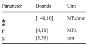
The first stage of the solution procedure was to calculate suit-able ranges for the 4-dimensional DOE, the small scale topog-raphy parameterψhas limits between 0 and 1 but the bounds of the small scale input parametersdp_dx;p;g needed to be iden-tified. To do this solutions to the smooth surface EHL problem were calculated using the same solver as described in

Section 3.2where the MLS metamodels were replaced by the basis functions with all coefficients equal to unity. The maximum/minimum values ofdp_dx;p;g were recorded at con-vergence and +/−10 % of the value added/subtracted to give the design space limits of each variable (negative film gaps and pressure are not permitted and were limited to 5μm and 0 Pa), the values were rounded and are presented in Table1.

The DOE was created using the bounds identified and the OLHC permutation GA of Bates et al. (2004). A DOE size of N = 1000 was selected as to ensure that the metamodel be accurate over the entire design space, high fidelity results were required over a fast computation because of the sensitivity of the large scale solver to the operating parameters. The justifi-cation of this number of points from the resulting metamodel accuracy is presented in Section4.2.

It is of note that the DOE was built in terms ofdp_dx;p;g;ψso that q,τ, p* were given as functions of these parameters but for the metamodel building and large scale solutiondp_dxand q were interchanged so thatdp_dx is a function of q, p, g,ψ. The relations forτand p* were not subject to this. In each of the three relations four of the five dimensions were structured such that they meet the space-filling criteria of the OLHC DOE. This ensures that when the MLS metamodels were cal-culated, the resulting approximation accuracy was not biased toward certain regions of the design space.

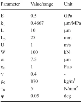
Each of the 1000 small scale simulations specified by the DOE were calculated and the outputs recorded. The values for all constants and operating conditions are given in Table2. COMSOL Multiphysics (COMSOL2015) was used to solve the range of small scale fluid structure interaction problems as defined in Section2.2. The MLS metamodels were then cal-ibrated by performing LOO-CV and k-CVon each of the three relations, the results produced were analysed and the optimal closeness of fit selected to within an acceptable significance. This was achieved using codes developed with MATLAB (MathWorks2015) as is also the case for remainder of the solution procedure described.

3.2 Large scale solution procedure

The large scale solution procedure began with an initial guess of zero pressure p, the undeformed film thickness h (specified by a minimum hb, pad length Lpand tilt angle φ) and an

arbitrary guess for the mass flow rate per unit depth q

Table 1 Bounds for the small scale input parameters

Parameter Bounds Unit

dp dx

[−40,10] MPa/mm

p [0,10] MPa

(constant along the length of the bearing (7)). The small scale topography parameter ψ was set to be constant along the length of the bearing. This was not a limitation to the method as it is conceivable that topography could vary along the pad length and indeed this variation could be parameterised and optimised in the same approach as described in Section3.3.

Two different methods were used to satisfy the boundary conditions for pressure (8) by treating the solution of the pres-sure gradient Eq. (6) either as an Initial Value Problem (IVP) or a Boundary Value Problem (BVP). The IVP method inte-grated (6) using the MATLAB function ode45 from the known inlet boundary condition of pa= 0, the error in the

outlet pressure boundary condition pb≠0 dictated whether q

had been over or under predicted. An iterative procedure was formed where q is increased if pb> 0 and decreased if pb< 0.

The BVP method used the MATLAB function bvp4c to spec-ify pa= pb= 0 and solves (6) and (7) together to give p and q.

This required a good initial guess for both variables, initially this was determined by solving the smooth surface pressure gradient equation with the IVP method as described above.

Once pb= 0 was satisfied to within a tolerance of 10−3the

large scale film gap g was updated according the deformation matrix operation (10). The load per unit area p* was assessed and relaxed (given an initial value of zero) with a factor of 0.5 to the previous iteration as to ensure convergence of g. After the new g was determined p and q were updated using the IVP or BVP methods, with the current values forming the new initial guesses. This continued until convergence in the pressure distribution was achieved, a tolerance of 10−3was required. Using the converged solution the shear stressτwas calculated. The load capacity W (5) and coefficient of frictionμ(4) were then recorded.

In order to ensure that the load capacity constraint (3) was satisfied a bisector approach was used, which is an appropriate method given that W reduces monotonically with increasing hb. Two values of hbwere selected and the corresponding W

calculated using the method as described above. A straight

line approximation was made from this W - hbrelationship

which is then used to predict the hbwhere Wreqwas achieved.

The limits of hbin the straight line approximation were

adjust-ed to include the new value and then the new W was calcu-lated. This process was repeated until convergence within a tolerance of 10−3in W was achieved.

3.3 Optimisation of small scale topography

In order to determine the value ofψwhich produced the mini-mumμfor the bearing a 1D bracketing optimisation approach was used (Forrester et al.2008). A parametric assessment ofμ was made over the full range of ψ. Any minima ofμ were identified from the response by the locations of where the de-rivative ofμwithψwas zero and the second order gradient was positive. These gradients were obtained by finite differences. The assessment ranges were refined around theψcorresponding to any minimum μ. The parametric assessment was repeated within these new limits and the process was repeated until the minimum value ofμconverged to within a tolerance of 10−3. After each iteration the ranges were refined by a factor of 0.5 around the new location of the minimum, unless this exceeded either of the initial bounds when that value was used instead.

4 Results and discussion

4.1 Design of experiments and metamodel building

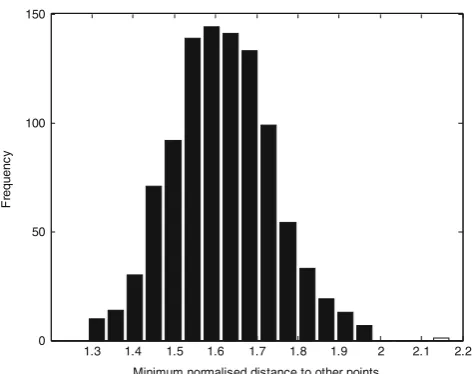
All results presented were calculated using a 6-core machine with 32 GB of RAM, running at 3.5 GHz. Figure3shows the frequency histogram of minimum normalised distance of each point to another point in the DOE. The range of minimum distances shown in Fig.3illustrates that the DOE is relatively well conditioned because the frequency distribution is close to normal and the variance is small, indicating that the OLHC has reduced the spread of the minimum distance to other points across all points in the domain. An outlier does exist and there is a slight skew in the distribution toward larger distances be-tween points. The size of the DOE (N = 1000) and the space-filling criteria of the OLHC ensures that there is enough infor-mation for the metamodel approxiinfor-mations to be accurate over the entire design space, as shown in Section4.2.

The process of running all 1000 small scale simulations took ~11 days of calculation. Cross validation for the MLS metamodel building was performed, the result of this for the pressure gradient metamodel is given in Fig.4.

Figure4indicates that the optimal closeness of fit for the pressure gradient metamodel obtained from k-CV (with k = 120) and LOO-CV are very close together, k-CV gives

θ= 39.09 and LOO-CV givesθ= 40.13. This shows that both cross validation methods can be used to perform accurate analysis of the closeness of fit response and that the best

Table 2 Constants and

operating conditions Parameter Value/range Unit

E 0.5 GPa

k1 0.4667 μm/MPa

L 10 μm

Lp 25 mm

U 1 m/s

W 100 kN

α 7.5 μm

η0 1 Pa.s

ν 0.4

-ρ0 870 kg/m3

τ0 5 N/mm2

closeness of fit for this DOE data is, to within an acceptable significance, 40. Similar conclusions can be drawn for the load per unit area and shear stress metamodels, in these cases the optimal closeness of fits were found to be 24 and 38 respectively.

Each LOO-CV procedure took less than 5 min to complete whereas the k-CV procedures took more than 2 h to run, this is because the k-CV method requires many more calls to the MLS assessment function than LOO-CV. It is therefore recommended that LOO-CV should be used for cross validation procedures of this type in the future since there is no benefit in accuracy from employing k-CV. This is different to the conclusions drawn by Loweth et al. (2011) who suggest that k-CV is a more accurate predictor in the context of their metamodels, their problem was however much smaller (N = 50) and therefore no noticeable dif-ference in computational time was observed. It is also shown in

Fig.4that the LOO-CV error is less than that given by k-CV. This is because the number of DOE points used in LOO-CV to build the validation metamodels is larger than that used in k-CV and therefore more in known about the response and a more accurate prediction is made.

4.2 Two-scale solutions and metamodel accuracy

Pressure and film gap distributions for three different values of the small scale topography parameter (ψ= 0.25, 0.5, and 0.75) are given in Figs.5and6respectively. These distributions are generated by solving the large scale problem as described in Section3.2(using both IVP and BVP methods) with the MLS metamodels created in Section4.1.

In order to validate the trends presented in Figs.5 and6

results generated at the large scale through the metamodel are compared against the exact corresponding small scale simula-tions. The mass flow rate as predicted by the large scale solver

0 10 20 30 40 50 60 70 80 90 100 0

1 2 3 4 5 6 7x 10

9

Closeness of fit

RM

S

E

k-fold Leave-One-Out k-fold min RMSE Leave-One-Out min RMSE

Fig. 4 Cross validation response for the MLS pressure gradient metamodel building

0 5 10 15 20 25

-1 0 1 2 3 4 5 6 7

x (mm)

p (

M

P

a)

ψ = 0.25 ψ = 0.5 ψ = 0.75

Fig. 5 Pressure distributions forψ= 0.25, 0.5, and 0.75

0 5 10 15 20 25

10 15 20 25 30 35 40

x (mm)

g (

μ

m)

ψ = 0.25 ψ = 0.5 ψ = 0.75

Fig. 6 Film gap distributions forψ= 0.25, 0.5, and 0.75

1.3 1.4 1.5 1.6 1.7 1.8 1.9 2 2.1 2.2 0

50 100 150

Minimum normalised distance to other points

Fr

e

q

u

e

n

c

y

is compared to the exact corresponding mass flow rate deter-mined at the small scale for three arbitrary locations (0, 10, 20 mm) along the distributions of pressure gradient, pressure and film gap. This check is performed for each ofψ= 0.25, 0.5, and 0.75 with the results tabulated in Tables3,4and5

respectively.

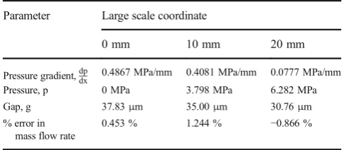
The absolute percentage error in mass flow rate predicted between the metamodel and exact small scale simulations is <4 % for all cases considered. This indicates that the MLS metamodel is accurately capturing the effects of the parameterised topography on the bearing performance. This also validates the choice in size and spread of the DOE used and implies that the subsequent optimisation procedure will lead to an accurate prediction of the best design. The largest % error is seen atψ= 0.25, here the result predicted is farther from the smooth surface model than for the remaining two cases (see the shape of the distributions given Figs.10and

13). This means that the underlying basis function of the metamodel has a poorer fit to the DOE data and the approxi-mation is therefore more likely to be less accurate in the region of the design space as it must deviate further.

Table6shows the time to compute for each of the threeψ specified using the IVP and BVP methods for solving the large scale governing equations of flow. The BVP method is shown to be approximately 45 % more efficient than the IVP method across all of the cases investigated, this method was therefore selected as the solution method to be used in the optimisation study. The time saving between the two methods represents a significant improvement from the method derived by de Boer et al. (2014). Table6also indicates that atψ= 0.25 the solution time for each method was much more than in the

other cases, this relates to the accuracy of the metamodel in this region of the design space and the influence of topography causing much larger deviations from the underlying functions of the MLS metamodel.

4.3 Optimisation of topography

Using the MLS metamodels validated in Section4.2, optimi-sation of topography was performed by the bracketing proce-dure outlined in Section3.3. The response and optimisation of

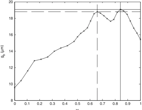
μwithψis presented in Fig.7, the minimum film gap gband q

corresponding to this are given in Figs. 8 and 9 (not all assessed points are displayed for the purpose of visualisation). The response shown in Fig.7 indicates that a transverse topography produces a lowerμ at constant W than purely longitudinal topography for the conditions investigated. This observation is consistent with that observed by Patir and Cheng (1978) when they conducted computer experiments using their flow factors approach to include the effects of topography in an EHL simulation. The response ofμwithψ is non-linear, asψincreases from 0 to 0.65 there is a decrease inμ from 0.023 to 0.08, between ψ= 0.65 andψ= 0.85μ remains between a value of 0.08 and 0.09, and asψincreases from 0.85 to 1,μincreases from 0.08 to 0.095. The optimisa-tion procedure took a total of ~15 h to converge, this accounted for 60 separate assessments ofμover the specified values ofψ.

Two local minima were identified by the optimisation pro-c e d u r e a t ψ= 0 . 6 5 7 9 a n d ψ= 0 . 8 4 2 1 f o r w h i c h μ= 8.104 × 10−3andμ= 8.028 × 10−3respectively. The mini-mum atψ= 0.8421 is therefore identified as the global mini-mum of μ for the conditions imposed and is therefore the optimalψfor the bearing design. Figures8and9show that

Table 3 Percentage error in mass flow rate forψ= 0.25

Parameter Large scale coordinate

0 mm 10 mm 20 mm

Pressure gradient,dp_dx 0.4302 MPa/mm 0.2700 MPa/mm −0.0714 MPa/mm Pressure, p 0 MPa 4.306 MPa 6.156 MPa Gap, g 34.27μm 32.33μm 27.11μm % error in mass

flow rate

−0.873 % 3.786 % 2.213 %

Table 4 Percentage error in mass flow rate forψ= 0.5

Parameter Large scale coordinate

0 mm 10 mm 20 mm

Pressure gradient,dp_dx 0.3658 MPa/mm 0.3633 MPa/mm 0.0221 MPa/mm Pressure, p 0 MPa 3.704 MPa 6.491 MPa Gap, g 35.71μm 32.77μm 29.06μm % error in

mass flow rate

1.198 % 1.997 % −0.225 %

Table 5 Percentage error in mass flow rate forψ= 0.75

Parameter Large scale coordinate

0 mm 10 mm 20 mm

Pressure gradient,dp_dx 0.4867 MPa/mm 0.4081 MPa/mm 0.0777 MPa/mm Pressure, p 0 MPa 3.798 MPa 6.282 MPa Gap, g 37.83μm 35.00μm 30.76μm % error in

mass flow rate

0.453 % 1.244 % −0.866 %

Table 6 Time to compute using the IVP and BVP methods

Small scale topography parameter

Time to compute IVP (s)

Time to compute BVP (s)

ψ= 0.25 2219 1330

ψ= 0.5 1032 573

a decrease inμleads to an increase gband q and an increase in

μleads to an decrease gband q, such that the minima

identi-fied forμcorrespond to maxima of gband q. Figures10and

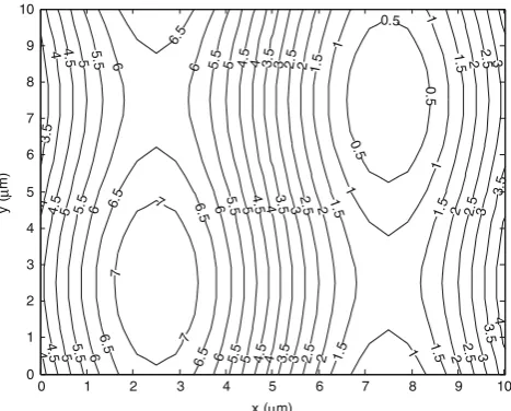
11illustrate the topography at the two minima identified. Given that the coefficients of friction calculated at

ψ= 0.6579 andψ= 0.8421 are similar it is interesting to note that they have very different features. In Fig.11the topogra-phy is dominated by transverse waviness, whereas in Fig.10

the topography is much more of a blend between transverse and longitudinal components. This highlights that the influ-ence of topography on friction is complex and that to describe and optimise the response ofμwithψthe two-scale method and subsequent metamodels are needed.

The coefficient of friction produced by the smooth surface model with the same parameters was found to be μ= 7.175 × 10−3. Simulations inclusive of topography predict-ed higherμ than the smooth surface equivalent. gband q

determined using the smooth surface model were found to be gb= 20.15μm and q = 0.01556 kg/s which are both higher

than any value determined with topography. These results show the potential of the multiscale approach for analysing the differences in bearing performance when topography is and is not considered. This subsequently demonstrates that when real surfaces are present the orientation of topography as manufactured can be guided by the optimisation process described. This method also provides a comprehensive frame-work for analysing and optimising surface topography in more complex cases which have been shown to have a role in re-ducing friction when compared to the smooth surface model, such as cavitating (Gao et al. 2015) and transient (Etsion

2005) lubrication.

The p,dp_dx, p*, g, andτdistributions for the textured bearing under load are shown in Figs.12,13,14,15and16at the two minima identified in Fig. 7 and directly from the smooth 0 0.1 0.2 0.3 0.4 0.5 0.6 0.7 0.8 0.9 1

0.008 0.01 0.012 0.014 0.016 0.018 0.02 0.022 0.024 ψ μ

Fig. 7 Response The coefficient of friction as a function of the small scale topography parameter

0 0.1 0.2 0.3 0.4 0.5 0.6 0.7 0.8 0.9 1 8 10 12 14 16 18 20 ψ gb (μ m)

Fig. 8 The minimum film gap as a function of the small scale topography parameter

0 0.1 0.2 0.3 0.4 0.5 0.6 0.7 0.8 0.9 1 0.004 0.006 0.008 0.01 0.012 0.014 0.016 ψ q ( k g/ s )

Fig. 9 The mass flow rate per unit depth as a function of the small scale topography parameter

0

.5 ₀.5

1 1 1 1.5 1.5 1. 5 1.5 1.5 2 2 2 2 2 2.5 2.₅ 2.5 2.5 2.5 2.5 2 .5 3 3 3 3 3 3 3 3.5 3. 5 3.5 3 .5 3.5 3.5 4 4 4 4 4 4 4 4 4 .5 4.5 4.₅ 4.5 4.₅ 4.5 4 .5 5 5 5 5 5 5 5 5 5.5 5 .5 5.5 5.₅ 5.5 6 6 6 6 6 6.5 6.5 6 .5 7 7 7

x (μm)

y (

μ

m)

0 1 2 3 4 5 6 7 8 9 10

0 1 2 3 4 5 6 7 8 9 10

surface model (without topography or fluid flow phenomena) respectively.

Figure12 shows that the pressure distributions obtained from the smooth surface model are similar in both shape and magnitude to that obtained with topography. Because the load capacity of each distribution is equal the differences in perfor-mance identified with topography cause only a small devia-tion from the smooth surface model in terms of pressure. This also implies that deviations in the pressure gradient will also be small and this is confirmed in Fig.13, these changes are small but the influence they have on the remaining part of the calculation is significant and the solution for each distribution is not trivial. The load per unit area shown in Fig.14indicates that this is almost identical to the pressure, where the differ-ence between these two distributions is orders of magnitude smaller than the pressure. The pressure distributions show that for the twoμidentifiedψ= 0.8421 produces a higher pressure

which occurs further toward the outlet of the bearing than for

ψ= 0.6579 and the pressure at ψ= 0.8421 is lower than

ψ= 0.6579 over most of the length of the bearing. This is an interesting observation because it indicates the difference in pressure distributions which result in similar coefficients of friction.

The film gap distributions presented in Fig. 15 show that a lower g is predicted for bearings with topography over the length of the bearing when compared to the smooth surface case. It is also observed that for the two topographies shown the shapes of the film gap distribu-tions are more comparable to each other than they are with the smooth surface model. Implying that with topog-raphy similar values ofμare given when the shape of the film gaps are also similar.

The film gap distributions presented in Fig.15show that with topography a lower g is predicted over the length of the 0.5 0 .5 0 .5 1 1 1 1 1 1.5 1 .5 1.5 1 .5 1.5 1. 5 2 2 2 2 2 2 2.5 2_.5 2.5 2 .5 2.5 2 .5 3 3 3 3 3 3 3.5 3_.5 3.5 3 .5 3.5 3.5 4 4 4 4 4 4 4 4 .5 4.5 4 .5 4.5 4_.5 4.5 5 5 5 5 5 5 5 .5 5.5 5 .5 5.5 5 .5 5.5 6 6 6 6 6 6 6.5 6 .5

6.5 6_.5

6.5

7

7

7

x (μm)

y (

μ

m)

0 1 2 3 4 5 6 7 8 9 10

0 1 2 3 4 5 6 7 8 9 10

Fig. 11 Contour plot of topography inμm at ψ= 0.8421 (global minimum)

0 5 10 15 20 25

-1 0 1 2 3 4 5 6 7 x (mm) p (M P a )

ψ = 0.8421 ψ = 0.6579 Reynolds

Fig. 12 Pressure distributions forψ= 0.6579, 0.8421 and the smooth surface model

0 5 10 15 20 25

-12 -10 -8 -6 -4 -2 0 2 x (mm) d p /d x ( MP a /mm)

ψ = 0.8421 ψ = 0.6579 Reynolds

Fig. 13 Pressure gradient distributions forψ= 0.6579, 0.8421 and the smooth surface model

0 5 10 15 20 25

-1 0 1 2 3 4 5 6 7 x (mm) p

* (N

/m

m

2)

ψ = 0.8421 ψ = 0.6579 Reynolds

bearing when compared to the smooth surface case. It is also observed that for the two topographies shown the shapes of the film gap distributions are more comparable to each other than they are with the smooth surface model. Implying that with topography similar values ofμare given when the shape of the film gaps are also similar. The film gap distribution given atψ= 0.8421 is lower thanψ= 0.6579 which indicates that under these conditions the minimumμfor a bearing with topography is synonymous with a minimum for the film gap over the length of the bearing.

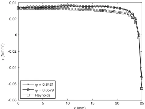
The shear stress distributions in Fig.16show that for bear-ings with topography included a larger value is predicted over the length of the bearing than in the smooth surface case, leading to large values ofμ. Both distributions with topogra-phy exhibit a similar shape and magnitude which explains why theμpredicted at theseψare also similar.

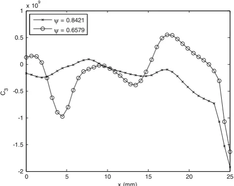
The MLS coefficients generated from the pressure gradient metamodel C1−3are plotted over the length of the bearing for

the two minima identified in Figs.17,18and19.

Each coefficient distribution represents how far from the smooth surface approximation (with C1−3= 1) the metamodel

deviates due to the influence of topography as determined by the small scale simulations. Figures17,18and19show that topography introduces a non-linear response for each coeffi-cient since there are no obviously identifiable trends in the responses over the length of the bearing. The coefficients pro-duced atψ= 0.6579 andψ= 0.8421 indicate that very differ-ent characteristics are introduced by the topographies and that in order to accurately model these effects the metamodel ap-proach is required. Also because the coefficient of friction produced by atψ= 0.6579 andψ= 0.8421 are close together and the MLS coefficients have no clear trends between them, this further implies that in order to conduct an optimisation study over a range of topographies that the two-scale method and subsequent metamodelling techniques are required.

0 5 10 15 20 25

15 20 25 30 35 40 45

x (mm)

g (

μ

m)

ψ = 0.8421 ψ = 0.6579 Reynolds

Fig. 15 Film thickness distributions forψ= 0.6579, 0.8421 and the smooth surface model

0 5 10 15 20 25

-0.08 -0.06 -0.04 -0.02 0 0.02 0.04

x (mm)

τ

(

N

/mm

2)

ψ = 0.8421 ψ = 0.6579 Reynolds

Fig. 16 Shear stress distributions forψ= 0.6579, 0.8421 and the smooth surface model

0 5 10 15 20 25

0.7 0.75 0.8 0.85 0.9 0.95 1 1.05 1.1 1.15 1.2

x (mm) C1

ψ = 0.8421 ψ = 0.6579

Fig. 17 MLS coefficient C1distributions forψ= 0.6579 and 0.8421

0 5 10 15 20 25

0.7 0.75 0.8 0.85 0.9 0.95 1

x (mm) C2

ψ = 0.8421 ψ = 0.6579

5 Conclusion

Surface topography influences the friction in lubricated sur-faces under load. Developing theoretical methods to optimise topography to, for example, minimise friction is complicated by the separation in scales between the size of the lubricated domain and the topography, the latter being at least an order of magnitude smaller. The separation in scales means that it is infeasible to computationally resolve the small scale features as well as the large scale bearing domain within a single computation.

The present study has shown how metamodels can be used within an efficient two-scale method to reduce friction in EHL bearings by optimising the small scale topography. Accurate metamodels are needed to represent the small scale data and it has been shown that combining OHLC DOE techniques with MLS metamodels that this can provide the accuracy needed. It is also found that there is very little difference between cali-bration of the MLS closeness of fit parameter using either the LOO-CV or k-CV methods and, given the significantly better computational efficiency of the former, LOO-CV is recom-mended for the calibration of the EHL metamodels. Note that this preference for LOO-CV over k-CV contrasts with the recent finding of Loweth et al. (2011) for much smaller sized data than is being used here. Another key finding is that the BVP method for determining pressure is over 40 % more efficient than the IVP method and offers a significant im-provement over the two-scale approach developed recently by de Boer et al. (2014). It is found that the MLS coefficients are strongly and non-linearly dependent on the topography and the EHL results show that very different topographies can lead to similar friction coefficients. Results also show further that, under a fixed load, transverse topography pro-duces a lower friction coefficient than longitudinal

topography, as is consistent with Patir and Cheng (1978), and this demonstrates that in order to optimise surface topog-raphy the two-scale method is required.

Acknowledgments The authors would like to thank the Engineering and Physical Sciences Research Council (Grant number EP/1013733/1) and the Leverhulme Trust (Grant Number F10 100/B) for funding this work.

Open AccessThis article is distributed under the terms of the Creative C o m m o n s A t t r i b u t i o n 4 . 0 I n t e r n a t i o n a l L i c e n s e ( h t t p : / / creativecommons.org/licenses/by/4.0/), which permits unrestricted use, distribution, and reproduction in any medium, provided you give appro-priate credit to the original author(s) and the source, provide a link to the Creative Commons license, and indicate if changes were made.

References

Abraham FF, Broughton JQ, Bernstein N, Kaxiras E (1999) Concurrent coupling of length scales: methodology and application. Phys Rev B 60(4):2391–2402

Audze P, Eglais V (1977) New approach for planning out of experiments, problems of dynamics and strengths, vol 35. Zinatne Publishing House, Riga, pp 104–107

Bates SJ, Sienz J, Toropov VV (2004) Formulation of the optimal latin hypercube designs of experiments. In Proceedings of the 45th AIAA/ ASME/ ASCE/ AHS/ ASC Structures, Structural Dynamics & Materials Conference. Palm Springs, USA

Benke M, Shapiro E, Drikakis D (2009) Modelling the polymer migration phenomena in DNA-laden flows. 2nd Micro and Nano Flows Conference, West London, UK

Breitkopf P, Naceur H, Rassineux A, Villon P (2005) Moving least squares response surface approximation: formulation and metal forming applications. Comput Struct 83:17–18

Cameron A (1971) Basic lubrication theory. Longman, London Choi KK, Youn B, Yang R-J (2001) Moving least squares method for

reliability-based design optimization, 4th World Congress of Structural and Multidiscpilinary Optimization, Dalian, China COMSOL (2015). User guide. [pdf] COMSOL. Avaliable at: (http://cdn.

comsol.com/documentation/5.1.0.234/COMSOL_ServerManual. pdf) [Accessed 1st October 2015]

de Boer GN, Hewson RW, Thompson HM, Gao L, Toropov VV (2014) Two-scale EHL: three-dimensional topography in tilted-pad bear-ings. Tribol Int 79:111–125

de Kraker A, van Ostayen RAJ, van Beek A, Rixen DJ (2007) A multiscale method modelling surface texture effects. J Tribol 129: 221–230

Dowson D (1999) History of tribology. Wiley, New York

Dowson D, Higginson GR (1966) Elastohydrodynamic lubrication: the fundamentals of roller gear lubrication. Pergamon, Oxford E W, Engquist B, Li X, Ren W, Vanden-Eijnden E (2007) Heterogeneous

multiscale methods: a review. Commun Comput Phys 2(3):367–450 Etsion I (2005) State of the art in laser surface texturing. J Tribol 127(1):

248–253

Forrester A, Sobester A, Keane AJ (2008) Engineering design via surro-gate modelling: a practical guide. Wiley, New York

Gao L, Hewson RW (2012) A multiscale framework for EHL and micro-EHL. Tribol Trans 55:713–722

Gao L, de Boer GN, Hewson RW (2015) The role of micro-cavitation on EHL: a multiscale mass conserving approach. Tribol Int 90:324–331 Gohar R (2001) Elastohydrodynamics, 2nd edn. Imperial College Press,

World Scientific, London

0 5 10 15 20 25

-2 -1.5 -1 -0.5 0 0.5

1x 10

9

x (mm) C3

ψ = 0.8421 ψ = 0.6579

Hewson RW, Kapur N, Gaskell PH (2011) A two-scale model for discrete cell gravure roll coating. Chem Eng Sci 66(16):3666–3674 Johnson KL, Tevaarwerk JL (1977) The shear thinning behaviour of

elastohydrodynamic oil films. Proc R Soc Lond A 356:215–236 Levin D (1998) The approximation power of moving least squares. Math

Comput 67:1517–1531

Loweth EL, de Boer GN, Toropov VV (2011) Practical recommendations on the use of moving least squares metamodel building. In Proceedings of the Thirteenth International Conference on Civil, Structural and Environmental Engineering, Chania, Crete, Greece, 2011, Civil-Comp Press

MathWorks (2015) User guide. [pdf] MATLAB. Avaliable at: (https:// www.mathworks.com/help/pdf_doc/matlab/matlab_prog.pdf) [Accessed 1st October 2015]

Patir N, Cheng HS (1978) Average flow model for determining effects of 3-dimensional roughness on partial hydrodynamic lubrication. J Lubr Technol Trans ASME 100(1):12–17

Rodkiewicz CM, Yang P (1995) Proposed Tehl solution system for the thrust-bearings inclusive of surface deformations. Tribol Trans 38(1):75–85 Roelands C (1966) Correlational aspects of the

viscosity-temperature-pressure relationships of lubricating oils, PhD thesis, Delft University of Technology, Delft, the Netherlands

Roux WJ, Stander N, Haftka RT (1998) Response surface approxima-tions for structural optimization. Int J Numer Methods Eng 42(3): 517–534

Sahlin F, Larsson R, Almqvist A, Lugt PM, Marklund P (2010) A mixed lubrication model incorporating measured surface topography. Part 1: theory of flow factors. Proc Inst Mech Eng J Eng Tribol 224(4): 335–351

Taflanidis AA, Jia G, Kennedy AB, Smith JM (2013) Implementation/ optimization of moving least squares response surfaces for approx-imation of hurricane/storm surge and wave responses. Nat Hazards 66:955–983

Toropov VV, Schramm U, Sahai A, Jones RD, Zeguer T (2005) Design optimization and stochastic analysis based on the moving least squares method, 6th World Congress of Strcutural and Multidiscpilinary Optimization, Rio de Janerio, Brazil

Tzeng ST, Saibel E (1967) Surface roughness effect on slider bearing lubrication. ASLE Trans 10(3):334–348