Location Awareness in Wireless Networks

(1)

Location Awareness in Wireless Networks

By

Barry Pearn B. Bus. (Accounting) Grad. Dip. App. Comp. A dissertation submitted to the

School of Computing

in partial fulfilment of the requirements for the degree of

Master of Computing by Coursework

(2)

Declaration

I, Barry Pearn certify that this thesis contains no material which has been accepted for the award of any other degree or diploma in any tertiary institution, and that, to the candidate’s knowledge and belief, the thesis contains no material previously

published or written by another person except where due reference is made in the text of the thesis.

(3)

Abstract

With the proliferation of wireless networks and the declining cost of wireless devices there is increasing interest in the development of location aware applications. These applications include robotics, context aware systems to collect or disseminate information, duress alarms in institutions such as hospitals and prisons and security of the wireless network.

There are many technologies that may be used to sense the location of mobile devices or personnel, including those based on infrared, ultrasonic, radio frequency tags and magnetic sensing. Most of these technologies require the deployment of devices specifically placed to support the location system. This paper focuses on a location system based on the RSSI of packets on the IEEE 802.11b wireless network. This technique has the great advantage that it may be implemented using off the shelf hardware that is generally already deployed to support the data network.

(4)

Acknowledgments

I would really like to thank Dr. Dan Rolf for supervising this research over the course of the year.

I would also like to thank the other staff and my fellow students at the School of computing for their advice and encouragement throughout the course.

I must also express my appreciation to Ekahau Inc, Sales Director Jarmo Ikonen and Andrew Curtis of Ekahau Australian distributor C1 Group for facilitating my research by allowing me an extended trial license of the Ekahau Positioning System.

(5)

List of Tables

Table 3-1 – Comparative standard deviation of reported RSSI for Broadcom and

Belkin cards in target devices ... 37

(8)

List of Figures

Figure 2-1 - Lateration to determine position in two dimensions... 17

Figure 2-2 - Angulation to determine a position in two dimensions. ... 18

Figure 2-3 - Active Mobile Architecture (based on Smith et al. 2004, p. 191) ... 21

Figure 2-4 - Passive Mobile Architecture (based on Smith et al. 2004, p. 191)... 22

Figure 3-1 - Estimated Indoor Free Path Loss ... 29

Figure 3-2 - Sensitivity of Path Loss Measurements ... 29

Figure 3-3 - Initial Wireless Network Configuration ... 34

Figure 3-4 - Revised Access Point Location... 35

Figure 3-5 - Sample of RSSI Reported by Belkin Card... 36

Figure 3-6 - Sample of RSSI Reported by Notebook (Broadcom card) ... 36

Figure 3-7 - Calibration Points ... 38

Figure 3-8 - Example Accuracy Summary... 38

Figure 3-9 – Example Graphical Error Display... 38

Figure 4-1 - RSSI recorded by Broadcom utility and NetStumbler... 38

Figure 4-2 - Test of free space path loss ... 38

Figure 4-3 – Overall error chart for initial 4 access point configuration ... 38

Figure 4-4 - Scatter plot of RSSI against distance to the AP... 38

Figure 4-5 - Effect of removing one access point when locating a static target. ... 38

Figure 4-6 - Plan of signal strength zones. ... 38

Figure 4-7 - Zone performance for mobile target ... 38

Figure 4-8 - Zone performance for static targets ... 38

Figure 4-9 - Typical error display for initial points in a mobile scan ... 38

Figure 4-10 - Effect of dropping first five points ... 38

Figure 4-11 - Errors on a static location ... 38

(9)

Figure 4-13 - Average pattern of convergence on fixed locations... 38

Figure 4-14 - Drift in indicated location at different times... 38

Figure 4-15 - Pattern of predicted locations at 15 Oct 8:24... 38

Figure 4-16 - Correlation of estimated distance with RSSI... 38

Figure 4-17 - Directional properties of notebook computer ... 38

(10)

Acronyms and Abbreviations

The following acronyms or abbreviations have been used in this paper:

AP Wireless Access Point

RSSI Received Signal Strength Indication.

(11)

1. Introduction

Recent advances in Wireless Local Area Network (WLAN) technology and falling costs of WLAN devices are expected to lead to a rapid increase in the proliferation of wireless networks. It has been predicted that there will be 39 million WLAN users worldwide by the end of 2004 and this number is predicted to grow to 120 million by 2008 (IT Facts.biz 2004). Market researchers, IDC were quoted (O’Brien 2004) to have predicted that the Australian market for LAN devices will “... double this year, growing 90 percent from $43 million in 2003.”

With the rapid growth of wireless networks there is a growing interest in techniques to determine the physical location of wireless devices. In traditional wired networks, networked devices ure usually situated in fixed locations that can be determined with reference to building plans and cabling diagrams. This is not the case with wireless networks. It is possible to determine the sub network to which a mobile device is attached. However, depending on the topology of the network this may reveal very little about the physical location of the mobile device and at best will only indicate that a device is within the coverage area of one or several wireless access points.

There are two main reasons why it could be advantageous to know the physical location of mobile computing devices attached to a network. The first of these reasons has to do with locating a mobile device for security, safety, maintenance or administration purposes. The second reason is to provide location information to the mobile device as part of a location aware application.

1.1 Security, safety and maintenance applications

(12)

WarDriving. These terms refer to the “recreational” use of scanning and monitoring tools to locate and map the locations of (especially) unprotected wireless networks. While such activities are often motivated simply by the technical challenge, the information collected may also be used to gain unauthorised access to networks either to obtain free access to the internet or to attack the private network for other more sinister purposes. Network administrators need to be concerned about such activities whatever their intended purpose. The ability to physically locate their source could be of great value in investigating and countering them.

In many industrial situations, personnel entering hazardous areas are required to place a tag in a location to indicate their presence. Procedures are implemented to ensure that machinery is not restarted until all personnel have retrieved their tag to indicate they are no longer in the hazardous area. In some complex environments it may be difficult to locate the owner of a tag. Valuable time may be lost while searching for personnel still in the area. A location system using responder tags that can be tracked by a location system could facilitate rapid location and evacuation of remaining personnel.

The increasing deployment of handheld IP telephones is another area where a location system could be of use. Traditional wired telephones are normally attached to a known fixed point so the origin of calls is reasonably easy to obtain. Handheld IP telephones though may be quite difficult to locate. If such phones were capable of being tracked by a location system, then the physical origin of calls could be

determined. Maintenance, security or any other personnel whose location is of interest could, if carrying a suitably equipped handset, be quickly summoned based on their current proximity to the site of an urgent task. Such a system could also support what are known as “enhanced 911” requirements to allow the source of emergency calls to be traceable.

1.2 Location aware applications

(13)

In data dissemination applications knowledge of the location of the mobile device can be used to modify the information it displays. An example of this type of application is a museum guiding application which can display information about exhibits in the current vicinity of the device and directions to various exhibits from the current location.. One such system, in the Marble Museum of Carrara, used PDAs and a location system based on infrared sensors placed throughout the display areas (Ciavarella and Patern 2004). Hospitals are another environment where context awareness can be of significant benefit. (Munoz et al. 2003) describes a hospital application where location and other context information are an important element of the system. A map based guidance system for locating books and collections has been implemented in the University or Oulu, Finland (University of Oulu 2003).

A location system could also be of benefit in data collection applications, especially with the in Wireless Sensor Networks where large numbers of sensors may be deployed across a target area. If these devices can determine their own location then the this can be reported with the sensor data.

Another application in which a location system could be of great benefit is that of duress alarms. The need for such a system was discussed by Christ and Godwin (1993). With location sensing incorporated in duress alarms, responding staff could be quickly directed to the correct location saving vital seconds. Location aware duress alarms could also have application in hospitals and other similar institutions

1.3 Overview

Chapter two of this paper presents a review of available research in the general area of indoor location systems, including their key properties, the choice of alternative techniques, technologies and architectures. Developments in the use of IEEE 802.11 Received Signal Strength Indication (RSSI) and techniques using Bayesian Filters are reviewed.

(14)

The detailed results and analysis of these tests is described in chapter four.

(15)

2. Literature Review

This chapter presents a brief review of the properties technologies and architectures to be considered when planning a location system and discusses research and developments in the field of location systems based on RSSI.

There are several technologies that can be used to provide location information in mobile networks. However before looking at particular technologies it is important to understand the issues that arise in discussing location systems.

2.1 Location system properties

A number of properties of location systems are considered by Hightower and Borrielo (2001b, pp. 57-60) as a basis for the discussion and consideration of location systems.

A location system may provide two types of information, a physical position or a symbolic location. A physical location is usually define by a set of co-ordinates in either two or three dimensions that define a particular point in space or on a surface such as a map or plan of a building. A symbolic location is a more abstract idea which can often be defined in relation to other objects or places. It may be said that a location is in a particular room, or in the vicinity of a particular door. Physical position is more precise as each location is unique whereas a location may be within more that one symbolic location.

A position may be referred to by an absolute reference or relative reference. An absolute reference places objects within a common frame of reference. For example the GPS navigation system gives position in terms of latitude and longitude and possibly elevation relative to sea level which is common to all such systems. On the other hand, a relative location is specified on a local frame of reference relative to some particular object of interest. Of course if the absolute location of two objects is known, then the position of one object relative to the other can be determined but in cases where the absolute position of both objects is not known, it may be sufficient to determine just their relative position with respect to each other.

(16)

system is an example. The satellite system provides the reference from which positions can be calculated, but knows nothing about the location of a particular device. The alternative is an infrastructure based system where the location is calculated by the system for use by the system or may be transmitted to the device. Localised computation may be required if privacy is an issue, but an infrastructure based system may reduce the power consumption and computational power required in the mobile

Two key properties of any location system are accuracy and precision. Accuracy refers to the granularity of the measurement, while precision is a measure of how often we expect to achieve a defined level of accuracy. The two are closely related and should be considered together. A system may be described as reaching an accuracy of 1 metre with a precision of 95 percent, meaning that positions within 1 metre of the true position will be reported 95 percent of the time.

Scale refers to the scope or range of a system and the number of mobile devices it can service. A system my provide locations within a room, throughout a building, across a campus or worldwide as in the case of GPS. The number of clients a system can support may be limited by computation power or network bandwidth or may be unlimited if mobile devices calculate their own positions.

A system may also need to deal with recognition of the identity of mobile devices. Such information may be useful where different mobile clients require different services.

Cost is an important property of any location system and may be measured in terms of capital outlays, time and such factors as bandwidth.

It is also necessary to be aware of the environmental limitations of the alternative systems. For example GPS systems do not work indoors and some RFID tagging systems my not work if more than a single tag is within range at once.

2.2 Location-sensing techniques

(17)

2.2.1 Triangulation

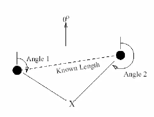
Triangulation is based on the geometric properties of triangles and can be further classified as lateration and angulation (Hightower and Borriello 2001a, pp. 1-5).

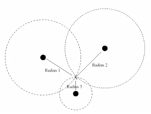
The term lateration refers to the technique used to determine a position from the intersection of distances measured from multiple known points. The basic technique is independent of the method used to measure the distances and could be equally used with physical

[image:17.612.196.448.305.496.2]

measurements, light beams, sound waves or radio signals and may use ‘time of flight’ or attenuation to indicate distance. To determine an unambiguous position in two dimensions requires measurement of distance from at least three non-collinear references as illustrated in Figure 2-1.

Figure 2-1 - Lateration to determine position in two dimensions.

The worldwide GPS system is perhaps the most widely known and used system based on triangulation using lateration.

(18)

[image:18.612.194.448.67.261.2]

Figure 2-2 - Angulation to determine a position in two dimensions.

An example of triangulation using angulation is the VHF Omnidirectional Ranging system used for aircraft navigation.

2.2.2 Proximity

Proximity location sensing is the technique of determining the location of an object by determining when it is near a known location. Proximity can be determined by detecting physical contact with pressure sensors or capacitive field detectors. In cellular phone networks and other wireless networks, location may be indicated by which base stations or access points the target is within range of. Proximity location also includes tracking a location by means of access tags, credit card point of sale transactions etc.

2.2.3 Scene analysis

Scene analysis as a technique for location sensing makes use of features of a scene observed from a location to draw conclusions about the location of the observer or objects in the view. The location is inferred by comparing the observed features of the scene with a dataset of observations from various known points of interest. A variation to this technique is differential scene analysis where movement is inferred from changes in the image.

(19)

2.3 Location systems technologies

Many different technologies have been proposed to solve the problem of location determination. A survey of the field in 2001 (Hightower and Borriello 2001b) listed a number of then current technologies.

2.3.1 Infrared technology

The Active Badge (Want et al. 1992) was a personnel location system developed by the Olivetti Research Laboratory (later absorbed by AT & T). This was a cellular proximity system based on the use of diffuse infrared technology. Each badge emits a globally unique identifier every ten seconds or on demand. Data is collected by a central server from infra red sensors distributed throughout the building and made available to applications through an application programming interface.

2.3.2 Ultrasonic technologies

Later work at AT & T produced the Active Bat system (Harter et al. 1999) which is a time of flight lateration system using ultrasound waves. The system used a large number of ceiling mounted ultrasound detectors which connected by a wired, daisy-chained network. The bats transmit ultrasound pulses in response to a radio signal from a controlling base station.

The Cricket Location Support System (Priyantha et al. 2000) is also an ultrasound system, combining both proximity and time of flight lateration techniques but reverses the method used in the Active Bat system by using active beacons to disseminate location information to listeners. Each beacon transmits a short string which conveys the semantics of the location it identifies. The located device contains software to calculate its own position from the ultrasound signal it receives.

2.3.3 Radio frequency systems

(20)

empirical method based on locating the nearest neighbour (or multiple nearest neighbours) in terms of signal strength. The second method, a signal propagation method used a

mathematical model of the indoor radio propagation environment to generate a theoretical model of the signal strength expected throughout the building. They found that the empirical model was more accurate, but the propagation model was more transportable and obviated the need for detailed calibration.

2.3.4 Magnetic tracking technology

Electromagnetic sensing is a technology that offers a position tracking method capable of a very high degree of precision (Hightower and Borriello 2001b). The technology is use in products that support virtual reality and motion capture for computer. An example is the MotionStar DC magnetic tracker produced by Ascension Technology Corporation (Ascension Technology Corporation 2004).

2.3.5 Computer vision technology

Several groups have explored using computer vision technology to determine the location of people or objects. For their Easy Living demonstration of an intelligent environment, Microsoft Research developed the Easy Living Tracker, which used images captured by multiple stereo cameras to track the movement of people (Krumm et al. 2000). The system was capable of tracking up to three people in a room. Easy Living is a visual scene analysis technology where the moving objects (people in this case) are recognised by the system. Visual scene analysis can also be applied in the opposite way where the visual environment is observed by the mobile object.

2.3.6 Physical sensor technologies.

(21)

2.4 Architecture of a tracking system

The architecture of a location system affects its scalability, ease of deployment and

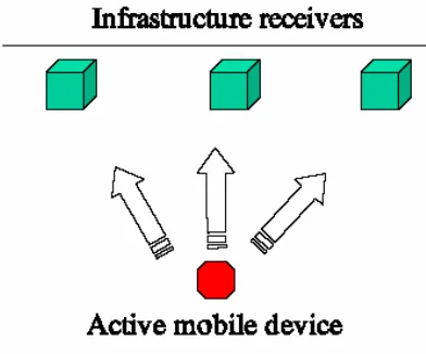
performance. Smith et al (2004, pp. 190-191) identify two main architectures for a location system, active mobile and passive mobile.

In an active mobile architecture, as illustrated in Figure 2-3, each mobile device periodically broadcasts a message on the communication channel. A number of fixed receivers are deployed throughout the area to be monitored and listen for these messages. The

[image:21.612.223.419.332.495.2]

characteristic of the signal that is used to estimate position is then sent to a central station which analyses the result and estimates the position. Depending on the nature of the system, the derived position can be passed back to the mobile device or to intrusion detection or other monitoring application.

Figure 2-3 - Active Mobile Architecture (based on Smith et al. 2004, p. 191)

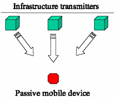
A passive mobile architecture uses a number of beacons deployed at known locations

(22)

[image:22.612.226.415.68.238.2]

Figure 2-4 - Passive Mobile Architecture (based on Smith et al. 2004, p. 191)

It was found that although the passive mobile architecture scales better with an increasing number of devices, it suffers some loss of accuracy compared with the active mobile

architecture because measurements are not made simultaneously. A hybrid architecture was proposed to preserve the scalability of the passive mobile system but provided increased precision of location (p. 201)

2.5 Choosing a location sensing technology

As has been demonstrated above, there are many different technologies to choose from when designing a location sensing system. They are each based on sensing different combinations of the properties outlined above and based on one or more of the three main sensing

techniques, triangulation, proximity sensing and scene analysis. The choice of a suitable technology for any planned application depends on the characteristics of the application and the environment.

For example, Ciavarella & Patern (2004) discuss the issue of choosing a technology to add location awareness to a PDA based museum guide application at the Marble Museum of Carrara. In this case, the material to be displayed was stored in the PDA environment and there was no requirement for network connectivity, so the requirement was only to determine the location of the device. Consideration was given to three alternative technologies,

(23)

In the case of the Marble Museum, this rather course grained proximity based approach satisfied the requirements of the application. Like many of the technologies considered above, this system required the installation of infrastructure specifically to support the location system.

On the other hand, the use of radio signal strength measurements for location sensing is unique among technologies considered in that it offers the possibility of using the existing wireless infrastructure installed for other purposes to provide location information. In situations where the devices to be tracked are Wireless LAN clients then a location system may be added with little or no additional outlay for hardware. Another advantage of

Wireless LAN sensing is that a system using standard devices can provide both location and identification information where other technologies can provide one or the other, but not both.

2.6 Using RSSI for location sensing

Because location sensing from observed RSSI has the key advantage that it can be achieved as a value added service using existing hardware, it is the main focus of this project. The techniques to be considered are based on the fundamental characteristics of radio signal propagation.

Wireless communication is possible because changes in the electron flow within a wire cause changes in the magnetic field surrounding the wire. Because these changes induce electron flows in other wires within the field a signal can be transmitted from one device to one or more remote devices. However only a very small fraction of the energy leaving the transmitting antenna ever arrives at the receiving antenna and this fraction becomes less as the distance between the two devices increases.

2.6.1 Limitations of RSSI measurement.

In theory it is possible to build an engineering solution to location sensing based on the properties of radio propagation by calculating the distances from a number of known access points and triangulating the position.

(24)

x The transmitted power of the Access Points may vary over time due to changes in environmental conditions such as temperature;

x The propagation characteristics of a building are non-uniform due to structural elements and fittings and may be subject to variation caused by environmental conditions or human activity;

x As discussed later in Par. 3.1, the sensitivity of RSSI measurements reduces rapidly at increasing distances and

x The RSSI reading obtained from some devices may be of limited precision (Par 3.1.2) and may fluctuate over time.

As a result of these problems, many researchers have been led to look for alternatives to the engineering solution of triangulating estimated distances.

2.6.2 Further work on using RSSI

Some of the earliest work to investigate the use of radio signal strength to estimate location of mobile stations was conducted in the Microsoft Labs (Bahl and Padmanabhan 2000b). RADAR, the system they developed was “ …based on an empirical signal strength measurements as well as a simple yet effective signal propagation model” (p. 10).

In a subsequent report (Bahl and Padmanabhan 2000a) examined some shortcomings in the basic version of RADAR and tested enhancements to improve the accuracy of continuous tracking, make the system more resilient to variations in the radio propagation environment and extend the algorithm to a three dimensional (multiple floor) space. The results obtained from the tests were encouraging. Their conclusion suggests further testing in real world environments and proposes the idea of deploying a larger number of “ light” access points which would only be used for location and have no other network function. Given the subsequent reductions in the cost of Access Points a higher density deployment of fully functional access point may be considered worthwhile to increase the level of redundancy and provide additional bandwidth.

(25)

laptop computer with a PCMCIA LinkSys wireless card to measure and record the received signal strength from wireless access points distributed throughout the building. Signal strength was determined by reading the measurement made by the card. The standard Linux kernel driver for the wireless card were modified to allow the scanning and recording of hardware MAC addresses and signal strengths in promiscuous mode. A Bayesian probabilistic model was used to predict the location of the mobile device. The system achieved one meter accuracy within one standard deviation and concluded that reliable localization can be achieved using wireless Ethernet

More recently a report by the same team (Ladd et al. 2004) apparently reporting on the same research noted that the observations reported were taken at night when the building was largely unoccupied. It was suggested that further work was needed to determine performance in more dynamic environments and suggested the need to look more closely at the placement of base stations. (Ladd et al. 2004, p. 558)

In later work by the same group in the same environment (Tao et al. 2003), an active mobile architecture was used to test modifications to the previous design aimed primarily at solving the specific problem of locating “ rogue” mobiles. In particular this was aimed to increase the robustness of the location algorithm if the target mobile deliberately changed its transmit power to try and mask its location.

In this case the hardware consisted of five “ snoopers” which were wireless enabled laptop computers that had custom built device drivers to read the signal strength from the receiver’s automatic gain control register. These were connected to a server which was a Java

application that collected the signal strength measurements from the snoopers and performed the statistical operation required to estimate the location of the target machine. The target machine was a laptop with a wireless card capable of varying it’s transmitting power. The conclusion reached was that using the modified technique it was possible to estimate the location of a mobile node that varied its transmit power.

In another study (Smailagic and Kogan 2002), four different algorithms based on signal strength measurements were compared:

(26)

x RADAR a system developed by Microsoft (discussed previously);

x CMU-PM which matches data collected by the mobile client against pre-generated tables of signal strength vectors.

x CMU-TMI used a polynomial function to calculate from signal strength the distance to each access point, derived a position in “ Signal Space” by intersecting the calculated distances and then made an adjustment from learned data

determine a position in “ physical space” .

They concluded that the CMU-TMI algorithm offered advantages in the reduced complexity of calibration and achieved a noticeable increase in accuracy.

The use of RSSI and proximity to estimate range between devices and sensor location and how both are affected by the random nature of fading were examined by Patwari and Hero (2003). It was found that RSS provided significantly more reliable estimates of location than proximity but that a quantized RSS using only three bits (8 levels of quantization) may be sufficient. This opens the possibility of reducing the complexity of the devices required (p. 28).

Some work at Rutgers University (Ganu et al. 2004) focussed on the use of infrastructure based “ sniffers” to monitor information about mobile clients and to support a server based location and security system. The purpose built sniffers operate in a passive mode and listen to the communication medium and timestamps and records the header information from the frame header of the management and control frames. The decoded information is forwarded to the centralised database for use by the location system.

2.6.3 Bayesian filtering

(27)

The application of Bayesian techniques to the problem of location estimation is discussed in some detail by Fox et al (2003b). Bayesian filters can be used to estimate the state of a system from a set of noisy observations. It was concluded that the use of Bayesian

techniques are “ … an extremely promising tool for location aware computing. The detailed analysis of Bayesian theory is beyond the scope of this study. Those interested in further exploration of the application of various Bayesian techniques such as Kalman Filters, Particle Filters and others as they apply to the area of location sensing are referred to more detailed analysis by Fox et al. (2003a; 2003b) and Ladd et al.(2004)

The use of statistical modelling approach to position estimation has also been pursued at the University of Helsinki (Tonteri 2001). Teemu Roos (formerly Teemu Tonteri), in a

subsequent paper, discussed the different machine learning approaches to the problem based on nearest neighbour and Bayesian algorithms. They found that “ … an average location estimation error below 2 meters is easy to obtain (p. 162). The Ekahau Positioning System which is discussed later in this paper is based on the Helsinki research.

2.6.4 Self correction

Because of the high sensitivity of location estimates to small changes in signal strength, changes in environmental conditions may cause locations estimated from RSSI data to “ drift” over time. This could be so whether the locations are derived by the engineering approach by triangulation, or by using a scene analysis approach using Bayesian or some other machine learning technique. Some work has been carried out to make such systems more robust in the face of variations in the signal propagation environment.

One approach is that of environmental profiling where multiple sets of data are recorded throughout the day and the base stations probe the environment periodically and pick a dataset on which to base the estimate (Bahl and Padmanabhan 2000a).

(28)

3. Methodology

This chapter begins with a brief discussion of the signal strength and how it is measured by a WLAN cards. It then discusses some software applications relevant to the area of interest. The final section describes the implementation of a location system in the School of Computing building.

3.1 Signal strength

3.1.1 Free-space path loss

The energy that is lost is called the free space path loss and can be calculated using the following formula:

PL = 32.4 + 20 log(f) + 20 log(d) (2-1)

Where PL is the path loss in decibels (dB), f is the frequency in MHz and d is the distance in km. (Unger 2003, p. 51) (But note that the formula as published by Unger contains an error – the first constant is printed as 92.4 and should be 32.4 and f is expressed in MHz, not GHz).

If we confine our consideration to the field of IEE 802.11 networks operating in the 2.4 GHz band then we can treat f as a constant and given the indoor environment take the distance in meters we can simplify formula (2-1) to:

PL = 40 + 20 log(d) (2-2)

It has been suggested elsewhere (Spread Spectrum Scene 2001) that the total path loss in a typical indoor environment is more typically given by the formula:

PL = 40 + 35 log(d) (2-3)

(29)

Indoor Free Path Loss

40.0 50.0 60.0 70.0 80.0 90.0 100.0 110.0 120.0

0 10 20 30 40 50 60 70 80 90 100

Distance (m)

Lo

ss

(d

B

)

(2-2) (2-3)

Figure 3-1 - Estimated Indoor Free Path Loss

What the curves in Figure 3-1 clearly illustrate is that as the distance of the transmission path increases, the amount of change in signal strength for a given change of distance decreases. This decrease in sensitivity is better illustrated in Figure 3-2 which shows the sensitivity of signal strength as an indicator of distance.

Sensitivity of Path Loss

0.00 1.00 2.00 3.00 4.00 5.00 6.00 7.00 8.00

0 5 10 15 20 25 30 35 40

Signal Path Distance (m)

Lo

ss

(d

B

/m

)

(2-2) (2-3)

Figure 3-2 - Sensitivity of Path Loss Measurements

(30)

distances. In a practical location system, signal strength will be measured by off the shelf networking components, not accurately calibrated laboratory instruments.

3.1.2 Signal strength measurements.

All IEEE 802.11 WLAN cards measure the RSSI continuously. The Physical Medium Dependent (PMD) sublayer returns a continual RSSI to the Physical Layer Convergence Procedure (PLCP) in the PMD service primitive PMD_RSSI.indicate. In the 802.11 Frequency Hopping Spread Spectrum system this is a four bit field with a range of values from 0 (weakest) to 15 (strongest) signal strength (Geier 2001, p. 133). Other 802.11 physical layer specifications (including 802.11 DSSS, 802.11a and 802.11b), use an eight bit field which allows 256 levels of signal strength (pp. 140, 149, 154). Both 802.11 Direct Sequence Spread Spectrum and 802.11b also optionally report signal quality in an eight bit primitive named PMD_SQ.indicate.

The RSSI is used by the PLCP for its clear channel assessment functions but, given suitable drivers, can be read by applications. Many adaptors are supplied with a configuration utility that includes the capability to display RSSI for the currently active channel or in some cases for all received channels. The RSSI indicator is implemented to provide necessary

information for the limited internal use of the WLAN system and there is no guarantee that it will provide precise measurement to external applications.

3.2 Software

There are several software packages and utilities available to measure, log and map WLAN signal strengths. While their interest is in locating and mapping wireless access points rather than finding the position of a wireless node, Byers and Kormann (2003, pp. 43-44) discuss some hardware and software issues that are relevant to the current problem. They include standard networking utilities and packages designed to discover and map WLANs such as NetStumbler and Kismet.

3.2.1 Site survey and WLAN utility tools

(31)

available access points. It works with many WLAN cards but depends on firmware and driver versions (Milner 2004). NetStumbler is a favoured tool of the warchalking sub-culture, but has uses in planning and configuring WLANs.

Kismet is an 802.11 layer two wireless network detector, sniffer and intrusion detection system. Kismet will work with any wireless card which supports raw monitoring (rfmon) mode, and can sniff IEEE 802.11b, 802.11a, and 802.11g traffic. Kismet identifies networks by passively collecting packets and detecting standard named networks, detecting (and given time, decloaking) hidden networks, and inferring the presence of non-beaconing networks via data traffic (Kismet 2004). Kismet will run on any operating system with Posix

compatibility (including Windows using Cygwin).

Wireless Research API (WRAPI) a software library that allows applications running in user space on mobile end stations to query information about the IEEE 802.11 network they are attached to. WRAPI 1.0 is implemented on the Windows XP operating system and is a hardware-independent tool that works with any IEEE 802.11b wireless network hardware vendor. WRAPI has been developed as a research tool by the University of California San Diego (USCD 2002)

WRAPI provides an interface to applications requiring information about the Wireless LAN. Many network card can be read and or modified using WRAPI.

3.2.2 Location software

A number of location and tracking systems are now either commercially released or under commercial development.

(32)

In operation, the Ekahau Site Calibration™ method is used for collecting radio network sample points from different site locations. Each sample point, containing station

identification, RSSI and the related map coordinates, is stored in the Positioning Model for use in location tracking. Ekahau Positioning Engine™ (EPE) is a positioning server that receives RSSI vectors from the client software on tracked targets and makes current location information available through an API for use by location aware applications. The software works with most industry standard access points and network cards.

WhereNet's WhereLAN Location Sensor and Locating Access Point combines location sensing features in a wireless access point. The Locating Access Point configuration delivers real time location sensing coverage plus an integrated wireless LAN access point to connect mobile workers to critical information. The devices receive and detect tag signals using “ … sophisticated digital signal processing.” (WhereNet) The Location Sensor and Locating Access Point are able to track a large number of WhereTags simultaneously to assure location accuracy over a very large coverage area. The Location Sensor and Locating Access Point forward tag signal information to the WhereNet Visibility Server Software where information can be graphically displayed, used for report generation, or accessed through the Internet.

WLAN Tracker (Komar and Ersoy 2004a; 2004b) is an experimental, software only system developed at the Bogazici University, Istanbul, that makes use of standard IEEE 802.11 WLAN hardware to provide location information for mobile wireless devices. Signal strengths from multiple Access Points are collected by the target device and sent to WLAN Tracker workstation for analysis. The system was tested outdoors and in a three story indoor environment.

3.2.3 HostAP and Linux

(33)

and possible also in IBSS. WPA and RSN (WPA2) is supported when used with accompanied tools, wpa_supplicant (WPA/RSN Supplicant) and hostapd (WPA/RSN Authenticator).

Intersil’s station firmware for Prism2 chipset supports a so called Host AP mode in which the firmware takes care of time critical tasks like beacon sending and frame acknowledging, but leaves other management tasks to host computer driver. This driver implements basic functionality needed to initialize and configure Prism2-based cards, to send and receive frames, and to gather statistics. In addition, it includes an implementation of following IEEE 802.11 functions: authentication (and deauthentication), association (reassociation, and disassociation), data transmission between two wireless stations, power saving (PS) mode signalling and frame buffering for PS stations. The driver has also various features for development debugging and for researching IEEE 802.11 environments like access to hardware configuration records, I/O registers, and frames with 802.11 headers (Malinen 2004).

HostAP opens up the possibility of constructing inexpensive access points with the capacity to listen to the network and collect signal strength information for use in estimating location of passive targets.

3.3 Implementation

3.3.1 Wireless network configuration

A test installation was established in the Main Block of the School of Computing building at the Newnham Campus of the University of Tasmania. There was no existing wireless network in the school and a preliminary survey of the wireless environment revealed only one low strength and infrequent signal from an adjacent building was detectable from inside the building.

(34)

network. An additional Access Point, a Belkin 6231-4, configured on channel 1, was used to provide an additional wireless signal, but was not connected to the Ethernet network.

Figure 3-3 - Initial Wireless Network Configuration

In this configuration, the three Airport Access Points were positioned at the corners of a triangle with the longest side of 37.5 metres so all points in the central area were within approximately 20 metres of at least two Access Points. The Belkin Access Point was initially placed in room V159 approximately equidistant from the other access points.

Preliminary testing revealed that this configuration did not produce consistent results. The estimated locations were erratic had large errors. On reflection it seemed that the problem arose because the three outer access points were too distant and the location of AP1, being located as it was did not add sufficient additional information when the target was at the extremities of the target area.

(35)

[image:35.612.167.475.69.236.2]

Figure 3-4 - Revised Access Point Location

A Hewlett Packard ze5730us Notebook Computer with an inbuilt Broadcom 802.11g

wireless LAN adaptor was used as the mobile target. The Ekahau software, (Client, Manager and Positioning Engine) were installed on this notebook.

A desktop computer with a wireless card was also configured and placed in Room V159. The Ekahau software was also installed on this machine and the positioning engine function was moved to this unit for the later tests. As well as providing a permanent host for the Positioning Engine for the duration of the tests, it was intended to use this fixed wireless node as a reference point to monitor the stability of the location estimates over time.

However, it was found that the estimated position for this unit was quite unstable. The RSSI indicators in the Ekahau Manager indicated a rapid fluctuation in the RSSI readings so it was suspected that this instability was caused by inconsistency in the measurement of RSSI reported by the WLAN adaptor.

(36)

85 90 95 100 9: 45 :0 0 A M 9: 45 :1 0 A M 9: 45 :2 0 A M 9: 45 :3 0 A M 9: 45 :4 0 A M 9: 45 :5 0 A M 9: 46 :0 0 A M 9: 46 :1 0 A M 9: 46 :2 0 A M 9: 46 :3 0 A M 9: 46 :4 0 A M 9: 46 :5 0 A M 9: 47 :0 0 A M 9: 47 :1 0 A M 9: 47 :2 0 A M 9: 47 :3 0 A M 9: 47 :4 0 A M 9: 47 :5 0 A M 9: 48 :0 0 A M 9: 48 :1 0 A M 9: 48 :2 0 A M R ep or te d R S S I ( N et st um bl er a rb itr ar y un its

[image:36.612.135.507.81.278.2]

) 11->stud-245 3->stud-245 7->stud-245

Figure 3-5 - Sample of RSSI Reported by Belkin Card

85 90 95 100 9: 45 :0 0 A M 9: 45 :1 0 A M 9: 45 :2 0 A M 9: 45 :3 0 A M 9: 45 :4 0 A M 9: 45 :5 0 A M 9: 46 :0 0 A M 9: 46 :1 0 A M 9: 46 :2 0 A M 9: 46 :3 0 A M 9: 46 :4 0 A M 9: 46 :5 0 A M 9: 47 :0 0 A M 9: 47 :1 0 A M 9: 47 :2 0 A M 9: 47 :3 0 A M 9: 47 :4 0 A M 9: 47 :5 0 A M 9: 48 :0 0 A M 9: 48 :1 0 A M 9: 48 :2 0 A M R ep or te d R S S I ( N et st um bl er a rb itr ar y un its

[image:36.612.133.511.336.533.2]

) 11->Pavilion 3->Pavilion 7->Pavilion

Figure 3-6 - Sample of RSSI Reported by Notebook (Broadcom card)

A more quantitative indication of this difference is obtained by calculating the standard deviation of the RSSI recorded for each signal path. As can be seen in Table 3-1, the

(37)

[image:37.612.200.446.109.213.2]

Table 3-1 – Comparative standard deviation of reported RSSI for Broadcom and Belkin cards in target devices

WIRELESS CARD

Channel _(Broadcom)Notebook _(Belkin)stud-245

3 1.09 3.68

7 1.10 5.97

11 1.09 3.92

The Belkin card was subsequently replaced with a Netgear model WG311 PCI Adaptor. While this provided a somewhat more stable indication of the predicted location of the (stationery) terminal, examination of the RSSI reading reported by NetStumbler showed more consistent readings for Access Point 3, but very erratic readings for Access Points 7 and 11 with frequent missed readings. In the NetStumbler log file both these access points frequently recorded an RSSI of -32618 (normal readings were in the range of 75-85 for access point 11 and 90-95 for access point 7).

Because of this difficulty, it seemed unlikely that any meaningful conclusions would be reached based on data from this machine and its use for this purpose was abandoned.

3.3.2 Calibration of the positioning system

The positioning system was then calibrated using the Manager application on the Notebook computer. Calibration was performed using a plan of the site which had been imported into the Manager application. The plan was scaled by selecting two known points and entering the known real world distance to set the scale in terms of pixels per unit (metres or feet). “ Tracking rails” were then drawn on to the plan to define the feasible paths within the area of interest. Calibration points were then recorded at intervals along these rails by indicating a location on the plan and rotating the device through a full circle to cancel out any directional effect of the mobile antenna. The manager records twenty samples of RSSI from each available access point.

(38)

[image:38.612.114.495.67.254.2]

Figure 3-7 - Calibration Points

3.3.3 Testing

The Manager application’ s built in Accuracy Analysis function was used with this calibrated model to record a total of 2667 points for subsequent analysis.

Points were recorded by clicking the current location on the on-screen plan then moving at a steady rate along a straight line and clicking further waypoints or an endpoint. True locations are interpolated between the indicated points assuming a steady rate of travel. RSSI vectors are recorded at regular intervals between the indicated points.

For each calibration run the manager application displays selected summary statistics for the accuracy achieved (Figure 3-8) and a graphical display of the error at each point (Figure 2-1).

[image:38.612.109.507.525.626.2]

(39)

[image:39.612.110.499.140.316.2]

The graphical display shows each point with an arrow indicating the direction and magnitude of the error in predicting that point. The head of the arrow indicates the position that was estimated for the point.

Figure 3-9 – Example Graphical Error Display

After recording this analysis with all available access points turned on it is possible to subsequently analyse the performance with different network layouts by selectively excluding one or more access points and then updating the accuracy analysis to show the location performance achieved with a subset of the full set of access points.

All of the data was recorded using the access point configuration shown in Figure 3-4. The data was collected using two different methods:

x Static Target

This is data collected at one of several known locations over a period of

approximately one minute for each session. A total of 1,624 separate observations were recorded during fifty three separate sessions. In each case, the session started and ended at the same location and comprised approximately thirty observations on the same fixed location.

x Mobile Target

(40)

walking speed averaged 0.73 metres per second within a range of 0.49 – 0.97 mps. Observations are recorded at intervals of two seconds giving between thirty two and sixty observations for each session and a total of 1,043 observations.

Summaries of the Accuracy Analysis results are included in Appendix A. The detailed data was exported from the manger program to text files and imported into a spreadsheet for further analysis. Both sets of data were analysed for the full four access point configuration as shown in Figure 3-4 and for a configuration using only AP3, AP7 and AP11 with AP1 disabled. A sample of the detailed data is included in Appendix B.6.

3.4 Summary

(41)

4. Results and Discussion

This chapter contains an analysis of the data collected from the various tests

undertaken and attempts to identify the configuration and environmental factors that affect the performance of the underlying method.

4.1 Measuring RSSI

Any system that uses signal strength to estimate location relies on the RSSI reading recorded by the wireless adaptor and the software used to read, display and record it. While the Ekahau manager software does display a dynamic bar chart of RSSI for all received access points, it does not have any facility to record the levels over time for external use. The Broadcom configuration utility provides a graphical display of RSSI and can log RSSI over time. NetStumbler displays signal strength in a bar chart form and store the data in memory. The stored data can be exported to a text file. The output from a sample of recorded signal with a single access point is shown in Figure 4-1. It should be noted that the Broadcom data is specified in dBm

(primary y axis) units while NetStumbler uses arbitrary RSSI units (secondary y axis). RSSI Measurement -60 -50 -40 -30 -20 -10 0

12:05:00 12:10:00 12:15:00 12:20:00 12:25:00

[image:41.612.156.516.459.660.2]

Time R S S I ( dB m ) 90 100 110 120 130 140 150 R S S I ( N et st um bl er a bi tr ar y un its Broadcom Netstumbler

(42)

The data sets are smoothed using a moving average and the secondary y axis scaled to match the two plots. While the point data of the two series show some quite wide variation, the smoothed data is comparable and indicates the scale units are similar with a level of 100 on the NetStumbler scale equating to –50 dBm as indicated by the Broadcom utility.

The variation in the reading of these two utilities of RSSI readings of the same signals from the same wireless card illustrates just one of the potential problems in obtaining accurate location prediction using these methods.

4.2 RSSI as an indicator of distance

In order to evaluate the relationship between distance and RSSI, some simple tests were conducted with the equipment used for the main study. The Belkin access point was set up in open space at a height of 600 mm. above the ground and signal

strengths recorded at various measured distances using the notebook computer positioned at a similar height. Signal levels were recorded concurrently using both NetStumbler and the logging feature of the Broadcom configuration utility. The data recorded by NetStumbler is displayed as a scatter plot in Figure 4-2.

RSSI to Distance

-60.0 -50.0 -40.0 -30.0 -20.0 -10.0 0.0

0 5 10 15 20 25 30 35 40

Distance to source (m.)

[image:42.612.154.491.469.643.2]

R S S I ( dB m ) 90 100 110 120 130 140 150 R S S I ( N et st um bl er a rb itr ar y un its ) Formula 2-2 RSSI Points Average RSSI

(43)

The plotted line in this chart is the predicted signal level using the free space path loss formula (2-2) and an arbitrary transmitted power level of +22 dBm. Signals were recorded for approximately one minute at each distance giving approximately forty samples at each location. The number of data points at each distance is not obvious because many may occupy the same position on the chart.

It can be seen that although there is a clear relationship between RSSI and distance, there is quite a large spread in the signal levels recorded at any one distance and the plot of mean levels displays significant deviations from the expected curve.

4.3 Location accuracy.

The key performance properties of a location system are accuracy and precision as outlined in Par. 2.1. Accuracy refers to the granularity of the measurement, while precision is a measure of how often we expect to achieve a defined level of accuracy. The two are closely related and should be considered together. The accuracy

requirements of a location aware application can be expressed in these terms. For example a particular application may require an accuracy of 1 metre with a precision of 95 percent, meaning that positions within 1 metre of the true position are required 95 percent of the time.

Data collected from a proposed location system operating under a given set of conditions can be analysed to calculate these properties which can then be directly compared with the stated requirements of the application. The result can best be summarised in a table showing the cumulative percentage of estimated locations that are within a given distance from the true location. The result is commonly displayed in the form of a chart.

(44)

both the static and mobile data using the final configuration of 4 access points as shown in Figure 3-4 is displayed in Figure 4-3..

Cumulative Error

0% 10% 20% 30% 40% 50% 60% 70% 80% 90% 100%

0 1 2 3 4 5 6 7 8 9 10

Error (metres)

C

um

ul

at

iv

e

P

er

ce

nt

[image:44.612.150.522.131.353.2]

Static Target Mobile Target

Figure 4-3 – Overall error chart for initial 4 access point configuration

It can readily be seen from this chart that, for example, approximately seventy seven percent of all estimated locations are within three metres of the true location. When tracking a mobile device, the error is less than five metres for ninety five percent of all observations. Interestingly only ninety percent of the observations of static targets are within five metres and the accuracy/precision in locating static targets is generally not as good as when tracking a moving target.

This initial assessment shows that this technique can provide potentially useful location information. However in many respects it raises more questions than it answers. These include question such as:

x What are the factors that limit the accuracy / precision of the estimates?

x Why is the accuracy / precision better when tracking a mobile target than simply locating a static one?

(45)

4.3.1 RSSI and distance

The known properties of radio frequency propagation allow the propagation loss in free space to be calculated. However propagation characteristics inside buildings are more complex. The walls and other structural element of the building, people and other objects all cause changes to the propagation of radio signal.

In order to further investigate the propagation characteristics of test environment, several samples of RSSI readings were collected. These were recorded using the logging function of the Broadcom Wireless Configuration Utility on the notebook computer. Several log files were recorded concurrently with the accuracy testing of the location system. These RSSI readings were then correlated by time in an Excel worksheet with the corresponding information exported from the accuracy analysis function in the Ekahau manager. Approximately 400 RSSI readings from the mobile tracking tests were matched up with the actual locations and plotted against the calculated distance to the relevant AP. The scatter plot is shown in shown in Figure 4-4.

RSSI at Various Distances

-80 -70 -60 -50 -40 -30 -20

0.000 5.000 10.000 15.000 20.000 25.000 30.000 35.000

Distance from AP

R

S

I (

dB

m

)

[image:45.612.158.510.427.627.2]

RSSI 1 RSSI 3 RSSI 7 RSSI 11 (2-2) (2-3)

Figure 4-4 - Scatter plot of RSSI against distance to the AP.

(46)

(100 mw). The curve 2-3 represents the modified formula proposed as an approximation of the theoretical loss inside buildings.

A number of conclusions can be drawn from Figure 4-4:

x There is a loose correlation between RSSI and distance to the transmitting AP but only within a broad band. Even for a single access point, the spread of recorded levels is generally wider than that recorded in the open (Figure 4-2). This is most likely a result of the effect of variation of attenuation caused by walls and other obstructions.

x This majority of plotted points conform roughly with the theoretical formulas with the upper limit generally at about the free path loss;

x The alternative formula (3-3) is a reasonable representation of the lower bound of the collected data and

x AP11 generally recorded a pattern of points clearly below the other units in RSSI at any given distance. As this access point was an identical model to AP3 and AP7 it seems likely that this difference is due to higher attenuation of intervening walls. No testing was undertaken to determine if this was so.

4.3.2 Number and spacing of access points

An obvious factor that would be expected to affect the operation of a location system is the density and location of the access points that are available to provide RSSI information. While the opportunity to change the location of the access points was limited it was possible to do some testing of this factor. In particular the location of AP1 was chosen so that it gave additional coverage of one end of the site but the area was reasonably well covered without it. The recorded test data for both the static and mobile tests were retested without AP1 in order to judge how much it contributed to the result.

(47)

subject to any change in environmental conditions. In fact the result when tracking the mobile client was almost identical so the overall accuracy was not affected by the presence or absence of the additional access point. On the other hand, the accuracy for location of a static target was affected as can be seen in Figure 4-5.

0% 10% 20% 30% 40% 50% 60% 70% 80% 90% 100%

0 1 2 3 4 5 6 7 8 9 10

Error (metres)

C

um

ul

at

iv

e

P

er

ce

nt

4 Access Points

[image:47.612.151.521.193.391.2]

3 Access Points

Figure 4-5 - Effect of removing one access point when locating a static target.

There is a reduction in accuracy of about 1 metre around the eighty percent precision level and a reduction of almost ten percent in the precision at an accuracy of three metres.

4.3.3 Zones of effectiveness.

(48)

[image:48.612.148.528.66.252.2]

Figure 4-6 - Plan of signal strength zones.

The signal strength plan clearly shows an area of superior coverage (minimum -60 dBm) in the centre of the target area with the signal pattern tapering off at both ends as one of the access points becomes more distant. To further investigate the effect of access point placement, the target area was arbitrarily divided into three signal strength zones as follows:

x Zone A is the area west of room V159 and is bounded by a line

approximating the -60 dBm signal contour. This area would be expected to be most affected by the presence of AP1.

x Zone B is room V159 and the adjacent hallways and approximates the area with greater than -60 dBm RSSI.

x Zone C is the area east of Zone B.

(49)

0% 10% 20% 30% 40% 50% 60% 70% 80% 90% 100%

0 1 2 3 4 5 6 7 8 9 10

Error (metres)

C

um

ul

at

iv

e

P

er

ce

nt

[image:49.612.151.521.99.300.2]

Zone A Zone B Zone C Zone A3 Zone B3 Zone C3

Figure 4-7 - Zone performance for mobile target

The zoned cumulative error chart for tracking of a mobile device (Figure 4-7) shows the performance in each of the three defined zones compared with the overall performance.

The performance in zone A shows a significant improvement compared to the overall result. This probably reflects the influence of the presence of access point 1 which ensures that most points in this area have reliable signals of reasonable strength from at least three well dispersed sources. Performance in zone B is closer to the overall result but still exhibits better performance at the higher end of the curve.

As would be expected the performance in zone C is considerably less accurate and this is clearly having a detrimental effect on the overall result. This may reflect the fact that access points one and seven are quite distant and access points seven and eleven are close to being co-linear at this end of the area and so do not provide much differentiation between locations.

(50)

0% 10% 20% 30% 40% 50% 60% 70% 80% 90% 100%

0 1 2 3 4 5 6 7 8 9 10

Error (metres)

C

um

ul

at

iv

e

P

er

ce

nt

[image:50.612.151.520.103.300.2]

Zone A Zone B Zone C Zone A3 Zone B3 Zone C3

Figure 4-8 - Zone performance for static targets

In Zone A the performance was almost identical to the overall result with all 4 access points active, but removal of the fourth access point had a significant impact. In Zone B, the performance was considerably better than the overall performance, with locations within 2.5 m. above 90% of cases. The impact of removing the fourth access point was noticeable, but had only a marginal effect on the performance curve. In Zone C the performance is again much worse and surprisingly having AP1 active resulted in a slight decline in performance.

Location Awareness in Wireless Networks