Mathematical modelling of granulation: static and dynamic liquid bridges

Mathematical Modelling of Granulation: Static and Dynamic Liquid

Bridges

Patrick Rynhart

I.F.S., Massey University, Palmerston North, New Zealand

[email protected]

R. McKibbin

I.I.M.S., Massey University Albany Campus, Auckland, New Zealand

[email protected]

R. McLachlan

I.F.S., Massey University, Palmerston North, New Zealand

[email protected]

J.R. Jones

I.T.E., Massey University, Palmerston North, New Zealand

[email protected]

Abstract

Liquid bridges are important in a number of industrial applications, such as the granulation of pharmaceuti-cals, pesticides, and the creation of detergents andfine chemicals. This paper concerns a mathematical study of static and dynamic liquid bridges. For the static case, a new analytical solution to the Young-Laplace equa-tion is obtained, in which the true shape of the liquid bridge surface is able to be written in terms of known mathematical functions. The phase portrait of the differential equation governing the bridge shape is then examined. For the dynamic case of colliding spheres, the motion of the bridge is derived from mass conser-vation and the Navier-Stokes equations. The bridge surface is approximated as a cylinder and the solution is valid for low Reynolds number (Re1). As the spheres approach, their motion is shown to be damped by the viscosity of the liquid bridge.

Introduction

Granulation is an important process in the powder industry [1]. The coalescence mechanism requires that fundamental particles be bound together with a viscous binder which is able to form a liquid bridge between particles. As a result of further inter-particle collisions, primary particles adhere together forming agglom-erates. As the granulation cycle continues, agglomerates bind together resulting in granules. This paper is concerned with the liquid bridges that form between fundamental particles. As an approximation, the parti-cles are represented by spheres in this work.

A number of theoretical studies have been completed into properties of static liquid bridges which have con-stant physical properties [2-7]. Parameters of interest in these applications are the critical rupture distance and the area and volume of the bridge. However, approximations to the true bridge shape are introduced to solve the problem. A well-known example of this is the toroidal approximation used by Fisher [5].

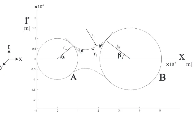
Figure 1: Illustration of the static liquid bridge geometry. Dimensional variables are used (as in equations (1) and (2)). A contact angle ofθ= 10o,α= 40o,β= 38o. The radius of particle A isrA= 0.1mm and particle BrB = 0.15mm.

The length of the bridge is0.12mm.

Static Bridges

Considerfigure 1 which illustrates a liquid bridge with cylindrical symmetry between two spherical particles ‘A’ and ‘B’ of radiirAandrB. Coordinatesrandxdefine the position of the liquid bridge surface along with the radii of curvaturer1andr2which lie in ther−xandr−yplanes respectively. The curvature

in ther-xplane is therefore given by 1

r1, and the curvature in ther-yplane by

1

r2. Allowing∆pto denote

the pressure deficiency caused by the presence of the liquid droplet (∆p >0when the internal pressure of the bridge is higher than the external (ambient) pressure), the Young-Laplace equation relates the surface tension of the binderγto the pressure difference∆pand the mean curvature of the bridge surface,

γ

1

r1

+ 1

r2

= ∆p. (1)

Gravity does not appear in (1) as the mass of the liquid bridge is very small in comparison with the surface tension force between particles. Upon substitution of the vector calculus results for r11 and

1

r2 (see [8] for

details), equation (1) can be written

γ

r

(1 +r2)3/2 −

1

r(1 +r2)1/2

=−∆p. (2)

Equation (2) can be non-dimensionalised by introducing variablesX =_σxandR= r_σ, whereσis the scaling variable relating non-dimensional and dimensional variables. In the case offigure 1,σcan be chosen as eitherrAorrB. Also, a non-dimensional pressure difference∆P = ∆_γp σ is introduced, enabling the non-dimensional version of (2) to be written as

R

(1 +R2)3/2 −

1

R(1 +R2)1/2 =−∆P. (3)

In (3) the notationR = dR

dX andR = d2R

dX2 has been adopted. Initial values for the bridge heightR0and

tangentR₀(occurring on particle A above) are specified. The angle which the bridge makes contact with the tangent plane to the spheres is thecontact angleθand is specified for a given problem. The starting value for the bridge height (occurring atX0) is

R0=

rA

and that of the slope at the point of contact is

R0= cot(α+θ).

Using the information above, an analytic solution to equation (3) is possible upon making the substitution

U =

1 +R2

−1 2

. (4)

DifferentiatingU with respect toX gives

dU

dX =−

RR

1 +R2

3 2

. (5)

Rearranging the right hand sides of (4) and (5), substituting these equations into (5) and applying the chain rule (where dU

dX dX dR =

dU

dR), (3) can be written as the followingfirst order differential equation,

dU

dR+

U

R = ∆P. (6)

Integrating (6) gives

U = R∆P

2 +

E

R (7)

where the constant of integrationEis the energy of the liquid bridge surface. Equation (3) defines a Hamil-tonian dynamical system and hence the energyEis conserved. By combining (4) and (7),

E=R

1

1 +R2 − R∆P

2 . (8)

Substituting (4) into (7) and rearranging givesRas

R= dR

dX =±

R2−∆P R2

2 +E

2

∆P R2

2 +E

Rearranging the above, the shape of the bridge (whereR0≤R≤R1) is given by the integral

X =

R

R0

∆P R2

2 +E

R2₋∆P R2

2 +E

2dR. (9)

IfE = 0then (9) can be solved to give

X2+R2=

2 ∆P

2

(10)

showing that the liquid bridge then has a spherical shape.

IfE = 0, (9) can be completed using integral tables [9]. The following parametric solution in terms ofX

is produced, X = F R ξ, χ

−F

R0

ξ , χ η+

2E

∆P η

+η E R0

ξ , χ

−E

R ξ, χ

0 0.5 1 1.5 2 2.5 3 3.5 4 4.5 5

−100

−80

−60

−40

−20 0 20 40 60 80 100

−1

−2

−3

−4

−5

−6

−7

0 0.1

0.2 0.3 0.4

0.5

R ∆ P

φ

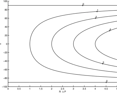
Figure 2: Phase portrait for∆P >0. Hereφ= arctanR. Contour labels are values ofE∆P.

where

η2, ξ2= 2 (∆P)2

(1−E∆P±√1−2E∆P

and

ξ=χ/η

such thatξ≤R≤η, and whereEandFare Jacobi elliptic functions of thefirst kind [9]. Equation (11)

de-fines the shape (R) of a bridge parameterised by the positionX, where the energy levelsEare determined from (8). Upon consideration of the discriminant of the the quadratic inX2 _{of (9), it can be shown that}

E∆P < 1₂.

Although equation (11) represents the liquid bridge configuration in terms of known mathematical functions, difficulty arises when attempting to integrate this solution to determine properties such as the bridge surface area and volume. In order to solve the problem in which certain properties are held constant, approximations to the bridge surface, or a numerical scheme, must be used (as in [2-6]).

Phase Portrait

The energy levelEis related to the height and slope of the bridge surface (R,R) by equation (8). Boundary conditions onRandR, along with the pressure difference∆Pdetermine the contour for a particular liquid bridge. Generic contours, characterising all liquid bridge configurations, can be obtained from (8) by scaling. Upon introducingR˜=R∆P andX˜ =X∆P, it follows that

E∆P = ˜R



 1

1 + ˜R2

−R˜ 2



. (12)

An angleφmeasured with respect to the horizontal coordinateXis introduced whereR= tanφand there-fore1 +R2= secφ. In terms ofφ, equation (12) becomes

E∆P = ˜R

cosφ−

˜

R

0 0.5 1 1.5 2 2.5 3 3.5 4 4.5 5

−100

−80

−60

−40

−20 0 20 40 60 80 100

1 2

3 4

5 6

7 8

9

10 0

0

R ∆ P

φ

(a) Phase portrait for∆P <0, in whichφ= arctanR is plotted againstR∆P. Contour labels are values of E∆P.

0 0.5 1 1.5 2 2.5 3 3.5 4 4.5 5

−100

−80

−60

−40

−20 0 20 40 60 80 100

0

0 1 2

3 4

R ∆ P

φ

(b) Phase portrait for∆P = 0. Labels are values ofE.

E∆P = ˜R

cosφ+

˜

R

2 for∆P <0 (13b)

and

E=Rcosφ for∆P = 0. (13c)

The phase portraits for equations (13a)-(13c) are shown infigures 2, 3(a) and 3(b). Thesefigures show that 5 distinct types of liquid bridges exist. With reference tofigure 2, forE∆P >0, periodic solutions exist for|φ| < 90o. For this case, the shape of the liquid surface is that of a ‘wavy’ cylinder. For the contour

E∆P = 0.5,φ ≡ 0o and this corresponds to the cylinder solution. ForE∆P < 0, the liquid surface begins with initial heightR0, and curves upwards reaching a maximum heightRmax > R0. The critical

contour atφ= 90o(E∆P= 0) is the sphere described in (10), which separates the cylinder and upwardly curved solutions.

When the pressure inside the bridge is equal to the external (ambient) pressure (as infigure 3(b)), two types of liquid bridges occur : for|φ| = 90o_{, the bridges start with initial heightR}

0and then curve inward

achiev-ing a heightRmin< R0. Forφ = 90o, the solution corresponds to two vertical planes separated byfluid.

When the pressure inside the bridge is lower than ambient (∆P <0), the bridges curve inward as shown in

figure 3(a).

Dynamic Bridges

Dynamic liquid bridges have previously been studied by Enniset. al[10]. Their study was directed towards establishing the relative importance of certain dimensionless groups which govern an axially strained dy-namic liquid bridge. We follow a different approach byfinding a vertically averaged pressure gradient for thefluid and then the subsequent bridge motion.

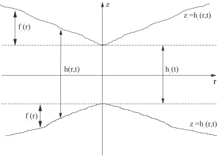
Theory is presented for two general surfacesz1(r, t)andz2(r, t), as shown infigure 4, with cylindrical

sym-metry about thezaxis separated by a gap distanceh(r, t). h0(t)is the closest approach distance between

the surfaces, andf1(r)andf2(r)describe the shape of each surface relative to a radial datum line occurring

atz=−h0(t)

2 andz=

h0(t)

2 .z= 0is defined to be midway between the closest approach points of the two

surfaces, which approach each other along thezaxis. The particular case for two approaching spheres with a constant bridge volumeV0, as illustrated infigure 5, will then be examined.

So that the dynamics can be studied, a simple approximation is made that the shape of the bridge is a cylin-der. Thefluid velocityv is assumed to be steady and at low Reynolds number (Re 1), implying that the inertial force is negligible in comparison with the viscous force of the bridge, and thefluid has constant viscosityµ. Thefluid has constant and uniform densityρ(as isothermalflow is assumed), and is isotropic and incompressible. Only viscous forces are studied. No other particle interactions, such as van der Waals, surface tension, electrostatics, or the body force effect of gravity are considered.

Balance Equations

Cylindrical coordinates(r, θ, z)are used, and the velocity vector isv = (vr, vθ, vz)wherevris the radial

fluid velocity,vθthefluid velocity about ther-zaxis, andvzthefluid velocity in thezdirection. For this system, the mass conservation equation from Hughes & Gaylord [11] is used,

1

r ∂

∂r(rvr) + ∂vz

∂z = 0 (14)

Neglecting inertial terms, that is assuming Re1, the momentum equations from [11] reduce to

0 =−∂P ∂r +µ

∂2_v

r

∂r2 +

1 r

∂vr

∂r + ∂2_v

r

∂z2 − vr

r2

(15)

0 =−∂P

∂z −ρg+µ ∂2vz

∂r2 +

1 r

∂vz

∂r + ∂2vz

∂z2

(16)

whereP = P(r, z)is the pressure difference between the inside and outside of the liquid bridge, defined to be positive when the pressure is higher internally. To make progress on this problem, an approximation thatvz vris introduced. Physically this means that the bridges must have a small volume, and that a small gap distancehmust separate the particles when compared to the volume and radius of a fundamental particle with radiusR. Sincevz vr, and because gravity is not considered in this approximation, only equation (15) is applicable to the solution.

Figure 4: Figure showing two general surfaces that are approaching each other, described byz1 =h1(r, t)andz2 = h2(r, t), separated by a distanceh0(t)which is the distance of closest approach between the two surfaces.

Velocity Pro

fi

le

Consider the volumeflow rateQoffluid displaced when surfacesz1andz2move toward each other. Since

the surfaces have cylindrical symmetry,

Q=

h2(r,t)

h1(r,t)

2πr vrdz. (17)

To determineQ, we manipulate (17) by taking the partial derivative ofQwith respect tor, and then dividing through byr. Upon completing this, we obtain

1 r

∂ ∂r

Z h2(r,t)

h1(r,t)

2πrvrdz

! = 2π

r

Z h2(r,t)

h1(r,t) ∂ ∂r(rvr)dz

+2π r

∂h2

∂r vr(r, h2(r, t), t)− ∂h1

∂r vr(r, h1(r, t), t)

(18)

where the second term in (18) arises upon application of the fundamental theorem of calculus and the chain rule. Now, since thefluid is unable to move through the surfaces,

Figure 5: The scenario in which two approaching equi-sized spheres, of radiusR, are connected together via a dynamic liquid bridge shown by the dotted lines.

This reduces (18) to

1

r ∂Q

∂r =

2π r

h2(r,t)

h1(r,t)

∂

∂r(rvr)dz. (19)

Substituting (14) into (19) yields

1

r ∂Q

∂r =−2π

h2(r,t)

h1(r,t)

∂vz

∂zdz

=−2π(vz(r, h2(r, t), t)

−vz(r, h1(r, t), t))

(20)

The separation functionsh1(r, t)andh2(r, t)can be written as the sum of a time dependent functionh0(t),

changing as the surfaces move, and a radial functionf1(r)andf2(r)as shown infigure 4. It is then possible

to writeh1(r, t) =−1₂h0(t) +f1(r)andh2(r, t) =1₂h0(t) +f2(r). Now

vz(r, h1(r, t), t) =

∂h1

∂t (r= 0, t) =−

1 2 ˙

h0(t)

vz(r, h2(r, t), t) =

∂h2

∂t (r= 0, t) =

1 2 ˙

h0(t),

so it follows that equation (20) is equivalent to

1

r ∂Q

∂r =−2π

1 2 ˙

h0(t)−−

1 2

˙

h0(t)

Therefore

Q(r, t) =−2π

r

0

rh˙0(t)dr=−πr2h˙0(t). (22)

For laminarflow, a parabolic radial velocity profile can be assumed,

vr(r, z, t) =A(r, t) [z−h1(r, t)] [h2(r, t)−z] (23)

whereA(r, t)is unknown andh1(r, t)≤z≤h2(r, t). Substituting (23) into (17) gives

Q=

Z h2(r,t)

h1(r,t)

2πr vrdz

=

Z h2(r,t)

h1(r,t)

2πrA(r, t) [z−h1] [h2−z]dz

= πr

3A(r, t) (h2(r, t)−h1(r, t))

3

(24)

Equating (24) with (22) gives the unknown functionA(r, t) = −3rh˙0(t)

h2−h1 , and the radial velocity profile is

therefore

vr(r, z, t) =−

3r[z−h1(r, t)] [h2(r, t)−z]

[h2(r, t)−h1(r, t)]

3 h˙0(t) (25)

Equation (25) is used tofind the pressure profile within the liquid bridge.

Finding the Pressure

Thermomentum equation (15) is used to consider the pressure. Rearranging (15) gives

1 µ ∂P ∂r = 1 r ∂ ∂r

r∂vr ∂r

+∂

2_v

r

∂z2 −

vr

r2 (26)

After differentiating (23) tofind ∂vr ∂r and

∂2_v

r

∂z2, and substituting these results in (26), we obtain, after some

tedious algebra, 1 µ ∂P ∂r =

−27_h4

∂h ∂r+ 36r h5 ∂h ∂r 2

−_h9r4

∂2_h

∂r2

z2h˙0

+ 18 h3 ∂h ∂r − 18r h4 ∂h ∂r 2

+6r

h3

∂2_h

∂r2

zh˙0

+6r ˙

h0

h3

(27)

which is valid for general surfaces described by a separation functionh. The radial pressure profile∂P ∂r for the case of equi-sized spheres of radiusRis obtained byfirst calculating the separation distance function

h(r, t), which is illustrated infigure 5. For spheres,

h(r, t) =h0(t) + 2(R−Φ)

whereΦ =√R2−_r2_.

Therefore

h(r, t) =h0(t) + 2

Differentiating (28) gives ∂h ∂r =

2r

√

R2_−r2 and

∂2_h

∂r2 =

2R2

(R2_−r2₎32. Substituting these into (27) gives

1 µ ∂P ∂r = ˙ h0

(R2−_r2₎32h3

54r3−72rR2

h z

2

+

;

28rR2−36r3z #

+ r

3

(R2−_r2_)h4 h

144 ˙h0z2−72zh˙0 i

+6r h3h˙0

(29)

Equation (29) includeszterms and this makes integration difficult tofind the pressureP. However, since thefluid layer is small in comparison toR, the vertically averaged pressureP¯provides an accurate approx-imation. Vertical averaging, given by

∂P¯

∂r =

1

h

h(r,t)

0

∂P

∂r dz, (30)

removes the explicitzdependence, and integration tofindP¯ is then straightforward. Substitution of (29) into (30) and integrating gives

∂P¯

∂r =

6rµ(R2+r2)

h3_(R2−_r2₎h˙0. (31)

If the pressure of the liquid bridge at somer=r0is at ambient pressurePamb, and then the bridge expands

tor > r0then vertically averaged pressure is

¯

P(r, t) =Pamb+ r

r0

∂P¯ ∂rdr

=P_amb+ 6µh˙0(t)

r

r0

r(R2_+r2₎

h3_(R2−_r2₎dr,

and the pressure difference

¯

P(r, t)−Pamb= 6µh˙0(t)

r

r0

r(R2_+r2₎

h3_(R2_−r2₎dr. (32)

Force

The pressure difference between the internal and external regions of the liquid bridge,P¯(r, t)−Pamb,

pro-vides the force which decelerates the particles.

The forceFbridgeis given by integrating the pressure difference over the cross-sectional area of the liquid

bridge. Using equation (32), the force is

Fbridge=m¨h0(t)

= Zr0

0

;_¯

P(r, t)−Pamb dA

= Zr0

0

2πrˆ

6µh˙0(t)

Zr

r0 ˆ

r(R2+ ˆr2)

h3_(R2_−rˆ2₎dr

r

dr drˆ

= 6πµh˙0

Zr0

0

Z r

0

2ˆr(R2_{+ ˆr}2₎

h3_(R2_−rˆ2₎r drdrˆ

−Zr0

0

r dr

Zr0

0

2ˆr(R2_{+ ˆr}2₎

h3_(R2_−rˆ2₎ drˆ

i.e.

¨

h0=

6πµh˙0

m {G(r0, h0)−

1 2r0

2_H(r

0, h0)} (34)

where the functions

G(r0, h0) =

r0

0

r

0

2ˆr(R2_{+ ˆr}2₎

h3_(R2_−rˆ2₎r dˆrdr

H(r0, h0) =

r0

0

2r(R2_+r2₎

h3_(R2−_r2₎ dr

(35)

are evaluated for current radiusr0and separationh0. Fourth order Runge-Kutta integration (Matlab’s ode45)

is used to evaluate the integrals on the right hand sides of (35). (Note that the functionhappearing in (35) is the separation function (28)). OnceGandHare evaluated, the bridge acceleration is determined using (34).

Numerical Solution

To maintain a constant liquid bridge volume ofV0, we specify a radiusrf correspondingh0 = 0(i.e. the

case where the spheres are touching). The volume to be maintained is then

V0=

rf

0

2πr

R−R2_−r2_dr

= R

√ R2_−r2

f

2πΦ (R−Φ)dΦ

where the substitutionΦ =√R2_−r2_{has been used. It follows that}

V0= 2π

1 3(R

2_−r2

f)

3 2 ₊1

2Rr

2

f − 1 3R

3

(36)

whereV0is the bridge volume.

The problem begins with the initial separationh0(0)specified. As the separation distance changes, the

cur-rent bridge radiusr0changes in order to maintain the constant volumeV0. Ifr0andh0are the bridge radius

and separation distance at timet, we are required to solve

V0= 2π

(R2_−r2 0)

3 2

3 +

Rr2 0

2 −

R

3

+πr2₀h0. (37)

For givenV0andh0there is a unique solution forr0which is determined numerically.

Equations (34) and (37) define a second order differential algebraic equation (DAE) subject to one constraint. Integration of (34) to obtain the bridge velocity and separation distance is achieved using a fourth order Runge Kutta integrator.

Depending on the initial values ofh0andh˙0, the liquid bridge exhibits four types of behaviour. Two cases

occur forh˙0 <0. If a small initial gap distance separates the particles, and provided the magnitude of the

initial velocityh˙0(0)is sufficient, then the particles will collide. However, since thefluid has no inertia,

energy is not stored in the liquid bridge and the particles do not rebound.

0 0.1 0.2 0.3 0

0.01 0.02 0.03 0.04

t

h0

0 0.1 0.2 0.3

−2.5

−2

−1.5

−1

−0.5 0 0.5

t

dh

0

/dt

0 0.1 0.2 0.3

0.56 0.57 0.58 0.59 0.6

t

r0

0 0.01 0.02 0.03 0.04

−3

−2.5

−2

−1.5

−1

−0.5 0

dh

0

/dt

h 0

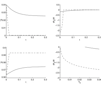
Figure 6: Two solutions from (34)-(37) are plotted for an initial separation ofh0(0) = 0.04mm. The solid line case

has initial particle velocityh˙0(0) =−0.2mm s−1, and the dashed line caseh˙0(0) =−2.2mm s−1.

equalising to that of external (ambient) pressure. Since no pressure difference exists across the liquid bridge, the bridge forceFbridge= 0(c.f. equation (34)) and no further particle movement occurs. Critical values for

the initial separation and velocity are a function of the parameters for the problem (such asR,mandµ).

Two cases occur when the particles are initially moving away, i.e. h˙0 > 0. Given this initial condition,

an escape velocityh˙∗exists such that ifh˙0(0) <h˙∗, the liquid bridge is able to retard the motion and the

particles will then come to a stop. Ifh˙0(0)≥h˙∗the particles continue to move apart.

An Example

Infigure 6 two examples are shown. The dashed line plot shows two spheres approaching, slowing, and colliding. The initial conditions used areh0(0) = 0.04mm andh˙0(0) =−2.2mm s−1. The solid line case

shows approaching spheres which do not collide, using the initial conditionsh0(0) = 0.04mm,h˙0(0) =

−0.2mm s−1_{. For both examples, the values of the parameters used areR = 1mm,r}

0 = 0.7mm,µ =

Nomenclature

Static

Variable Description Units

r Vertical coordinate m

x Horizontal coordinate m

y Bridge coordinate m

θ Contact angle o

α Half angle for particle ‘A’ o β Half angle for particle ‘B’ o

∆p Pressure difference Pa

σ Scaling variable m

R Non-dimensional bridge -vertical coordinate

X Non-dimensional bridge -horizontal coordinate

∆P Non-dimensional

-pressure difference

E Energy level

-Dynamic

Variable Description Units

r Vertical coordinate m

R Sphere radius m

z Vertical Coordinate m

h Separation function m

h0 Closest separation m

v Velocity vector m s−1

ρ Fluid density kg m−3

g Acceleration due to gravity m s−2

µ Dynamic Viscosity kg m−1

P Pressure within liquid bridge Pa

Pamb Ambient pressure Pa

¯

P Vertically averaged pressure Pa

Re Reynolds number

-Fbridge Force N

V0 Constant bridge volume m3

References

[1] Sherrington P J and Oliver R.Granulation. Heyden and Sons Ltd, 1981. London.

[2] Erle M A, Dyson D C and Morrow N R. Liquid bridges between cylinders, in a torus, and between spheres.AIChE Journal, 17(1):115–121, 1971.

[3] Lian G, Thornton M J and Adams M J. A theoretical study of the liquid bridge forces between two rigid spherical bodies. Journal of Colloid Interface Sciences, 161:138–147, 1993.

[4] Simons S J R and Seville J P K. An analysis of the rupture energy of pendular liquid bridges.Chemical Engineering Sciences, 45:2331–2339, 1994.

[6] Willett C D, Adams M J, Johnson S A and Seville J P K. Capillary bridges between two spherical bodies.Langmuir, 16:9396–9405, 2000.

[7] Batchelor G K.An Introduction to Fluid Dynamics. Cambridge Univerisity Press, 1967. Cambridge. [8] Hsu H P.Applied Vector Analysis. Harcourt Barace Jovanovic, 1984. Florida USA.

[9] Gradshteyn I S and Ryzhik I M.Table of Integrals, Series and Products. Academic Press, 1980. [10] Ennis B J, Tardos G , Pfeffer R. The influence of viscosity on the strength of an axially strained pendular

liquid bridge.Chemical Engineering Science, 45(10):3071–3088, 1990.