M. Campos Pinto and F. Charles, Editors
ELECTROMAGNETIC PIC SIMULATIONS WITH SMOOTH PARTICLES: A
NUMERICAL STUDY
∗Martin Campos Pinto
1, Mathieu Lutz
2and Marie Mounier
3Abstract. In this article we study a charge-conserving finite-element particle scheme for the Maxwell-Vlasov system that is based on a div-conforming representation of the electric field and we propose a high-order deposition algorithm for smooth particles with piecewise polynomial shape. The numerical performances of the method are assessed with an academic beam test-case, and it is shown that for an appropriate choice of the particle parameters the efficiency of the resulting method overcomes that of similar finite-element schemes using point particles.
R´esum´e. Cet article pr´esente un sch´ema ´el´ements-finis conservant la charge pour le syst`eme de Vlasov-Maxwell bas´e sur une repr´esentation div-conforme du champ ´electrique, ainsi qu’un algorithme d’ordre ´elev´e pour d´eposer le courant port´e par des particules r´eguli`eres polynˆomiales par morceaux. Les performances num´eriques du sch´ema coupl´e sont ´evalu´ees `a l’aide d’un cas test acad´emique de faisceau, et nous montrons que pour un choix appropri´e des param`etres des particules, cette m´ethode se r´ev`ele plus efficace que d’autres sch´emas similaires coupl´es avec des particules ponctuelles.
Introduction
We consider a numerical scheme for the 2D Transverse Electric (TE) Maxwell system
∂tE−c2curlB=−1
ε0J (1)
∂tB+ curlE= 0 (2)
coupled with a Vlasov equation to model the transport of particles with elementary chargeqand massm,
∂tf+v·∇xf + q
m(E+v×B)·∇vf = 0. (3)
Heref =f(t,x,v) is the plasma distribution function in phase-space, with x= (x, y) the position variable,
v = (vx, vy) the velocity variable. In the above TE mode, the electromagnetic field takes the form E =
(Ex(x, t), Ey(x, t)),B=Bz(x, t) and the 2D reduction yields two curl operators, namely
curlB= (∂yB,−∂xB) and curlE=∂xEy−∂yEx,
as well as two vector product operators: one acting on a pair of vectors (u,w) inR2 seen as vectors inR3 with vanishing third component, and another one acting on a pair (u, w) whereu is again a vector in R2 seen as the vector (ux, uy,0)∈R3, and wis a scalar seen as the vector (0,0, w)∈R3. Thus, it yields
u×w=uxwy−uywx and u×w= (uyw,−uxw).
∗ An important part of this work was carried out in the Congapic project during the Cemracs 14 research session, with
funding support from the AMIES agency.
1 CNRS, Sorbonne Universit´es, UPMC Univ Paris 06, UMR 7598, Laboratoire Jacques-Louis Lions, 4, place Jussieu 75005,
Paris, France
2 Universit´e de Toulouse, UMR5219, Institut de Math´ematiques de Toulouse, F-31062 Toulouse, France 3 Nucl´etudes, CS 70117, 91978 Courtaboeuf cedex, France
c
EDP Sciences, SMAI 2016
Finally the charge and the current density are given by
ρ(t,x) :=q Z
R2
f(t,x,v) dv, (4)
J(t,x) :=q Z
R2
vf(t,x,v) dv (5)
and we recall that they satisfy a continuity equation
∂tρ+ divJ = 0. (6)
As is well known and formally verified by taking the divergence of the Amp`ere equation (1), this property of the source guarantees that the solutions of the above Maxwell evolution system satisfy the Gauss law
divE = 1
ε0ρ (7)
at any time t, as long as it is the case for the initial solution E0. (For the magnetic field the Gauss law is degenerate since B=Bz(x, t) has a zero divergence by construction.) The aim of this article is to describe
a FEM-PIC scheme with smooth particles for the above Maxwell-Vlasov system that is charge-conserving in the sense that it preserves a (strong) Gauss law for the numerical solution, and to study its numerical performances with an academic beam test-case.
The outline is as follows. In Section 1 we describe a mixed finite-element method for the time-dependent Maxwell system (1)-(2) that is based on a div-conforming representation of the electric field E, and we recall the particle approximation of the Vlasov equation (3). In this charge-conserving scheme the current is discretized using a Raviart-Thomas interpolation that is recalled in Section 2.1, and in Sections 2.2 and 2.3 we describe how to apply it using numerical Fekete quadratures in the case whereJ is approximated by smooth particles. Finally we show in Section 3 some numerical results obtained for a smooth electron beam in a simple domain. In particular, we discuss how the accuracy and efficiency of the resulting FEM-PIC scheme vary with some parameters of the smooth particles, and we compare it with two FEM-PIC methods using point particles.
1.
Description of the numerical scheme
In the present Section we describe the numerical method used to simulate the Maxwell-Vlasov system. We consider a bounded computational domain Ω with Lipschitz boundary that is partitioned by a regular family of conforming simplicial meshes (Th)h>0, and inside each triangleT ∈ Thwe assume that the vertices
{xT
0,xT1,xT2}are numbered counterclockwise. We denote the corresponding edges byE(T) ={eT0, eT1, eT2}, so
thateT
i andxTi are opposite. We also letnTe be the outward unit vector ofT that is normal toe, andτTe the
associated tangent vector obtained by rotating nT
e through + 90 degrees. We then write Eh=∪T∈ThE(T) and assuming that the triangles are given arbitrary indices, we fix an orientation for the edges as follows. For any e∈ Eh, we letT−(e) be the triangle of minimum index for which e is an edge. If e is shared by
another triangle we denote the latter byT+(e). Note that, due to the conformity of the mesh, no more than
2 triangles can haveeas an edge. The edgeeis then oriented by setting
xe0:=xT −(e) i+1 , x
e 1:=x
T−(e)
i+2 whereiis such thate=e T−(e)
i (8)
(and where for simplicity we have identifiedxTi−(e) andxTi+3−(e)). We also set
ne:=nT −(e) e ,
and observe that ifeis an interior edge then we havene=−nTe+(e). We denote by ˆT a reference triangle
with vertices
ˆ
x0:=
0 0
, x1ˆ :=
1 0
, x2ˆ :=
0 1
and we let
FT : ˆT →T, xˆ 7→xT0 +FTxˆ, FT := xT
1 −xT0 xT2 −xT0 yT
1 −yT0 y2T −y0T
(9)
be the affine function that maps ˆT on anyT ∈ Th(and preserves the numbering of the vertices). As for the
boundary conditions, we will consider standard metallic and Silver-M¨uller boundary conditions, namely
n×E=
(
0 on the metallic boundaries ΓM ⊂∂Ω
n×(n×cB) =cB on the absorbing boundaries ΓA=∂Ω\ΓM
(10)
wherenis the outward unit vector normal to∂Ω.
1.1.
Finite element scheme for the Maxwell system
For the Maxwell system we consider a space discretization that relies on a mixed formulation with a strong Amp`ere equation. It involves a continuous finite-element space for the magnetic field
Vhµ:=Pp(Th)∩H(curl; Ω) =Pp(Th)∩H1(Ω) ={u∈ C(Ω) :u|T ∈Pp(T), T ∈ Th} (11)
where Pp(T) denotes the space of polynomials of total degree ≤pon T (note that the spaces H(curl; Ω)
andH1(Ω) coincide in 2D), and a div-conforming Raviart-Thomas finite-element space for the electric field
Vhε:=RTp−1(Ω,Th) ={u∈H(div; Ω) :u|T ∈ RTp−1(T), T ∈ Th} (12)
with RTp−1(T) :=Pp−1(T)2+ x
yPp−1(T) see e.g. [1, 4] for further details on H(div) conforming spaces.
Here the exponentsµandεstand for “magnetic” and “electric” respectively. In a semi-discrete setting, the approximate electro-magnetic field is then defined as the solution (Bh(t),Eh(t))∈V
µ h ×V
ε
h to the system
(h∂
tBh, ϕi+hEh,curlϕi+chBh, ϕiΓA= 0 ϕ∈V µ
h ⊂H(curl; Ω)
h∂tEh,ϕi −c2hcurlBh,ϕi=−ε10hJh,ϕi ϕ∈V
ε
h ⊂H(div; Ω)
(13)
whereJh∈Vhε is an approximate current density. This discretization is of course not new. Its convergence
is established in [8] (for the 3D Maxwell system) and its charge conservation properties are advocated in [9], where it is presented as a “D/H formulation” due to the fact that it essentially relies on representing the electric field (and the current density) as a 2-form defined through its fluxes.
This discretization has several interesting properties. First, using the embedding curlVhµ ⊂Vε h we see
that the discrete Amp`ere equation holds in a strong (i.e., pointwise) sense inVε h
∂tEh−c2curlBh=−ε1
0Jh, (14)
and for this reason we may call (13) a “strong-Amp`ere” discretization. Second, we observe that if Jh is
defined as
Jh:=πhdivJ (15)
where πdiv
h is the finite-element interpolation on the Raviart-Thomas space V ε
h (see Section 2), then the
approximate electric field satisfies a (strong, i.e., pointwise) Gauss law involving an approximate charge density. Indeed, as can be verified with integrations by parts, the finite-element interpolation satisfies a commuting diagram property
divπhdivu=Phdivu, u∈H1(Ω) (16)
wherePh:L2(Ω)→Pp−1(Th) is theL2-projection on the piecewise polynomials of degree≤p, i.e.,
hPhu, ϕi=hu, ϕi, ϕ∈Pp−1(Th).
In particular, taking the divergence of the strong Amp`ere equation (14) and using the continuity equation (6) yields
divEh= 1
ε0 ρh
Remark 1.1. We observe that the electric fieldEhcan be computed in a discontinuous spaceV˜ε
h containing Vε
h, indeed the discrete Amp`ere equation holds in a strong (i.e., pointwise) sense, so that the electric field Eh will belong to thediv-conforming Raviart-Thomas spaceVε
h as long as its initial valueEh does so. Remark 1.2. A probably more usual finite-element discretization of the TE Maxwell system(1)-(2)consists of looking for Eh(t)in acurl-conforming space VhεandBh(t)in a spaceV
µ
h containingcurlV ε
h, such that
h∂tEh,ϕi −c2hBh,curlϕi+chn×Eh,n×ϕiΓA =− 1
ε0hJh,ϕi ϕ∈V
ε
h ⊂H(curl; Ω)
h∂tBh, ϕi+hcurlEh, ϕi= 0 ϕ∈Vhµ⊂L2(Ω).
(17)
Such a discretization may be called “strong-Faraday”, as it leads to a Faraday equation being satisfied point-wise by the discrete solutions. Compared to (13), an explicit time discretization based on (17) leads to inverting at each time step a mass matrix in acurl-conforming space (forEh) instead of acurl-conforming space (for Bh). Because the former consists of vector-valued fields, it results in more expensive solves. We note that this advantage is lost in 3D, since both the electric and magnetic fields have their values in R3.
There, the differences of the “strong-Amp`ere” and “strong-Faraday” discretizations essentially lie in the type of degrees of freedom that are used to determine the discrete fields, and in the proper approximation operators that one should use for the current density, as described in [3].
1.2.
Particle method for the Vlasov equation
The Vlasov equation (3) is discretized by a particle method which consists of approximating f by a collection ofN numerical particles,
fN(t,x,v) := N X
k=1
ωkS(x−xk(t))S(v−vk(t)). (18)
Here the shape functionS can either be a Dirac measure or a smooth, symmetric function (S(−v) =S(v)) with compact support and unit integral. As for the phase-space particle centers (xk,vk), they are initialized together with the particle weightsωk in such a way that fN(t = 0) approximates the initial data f0 in a
function or in a measure’s sense, and they are transported by following the characteristic curves associated to (3), i.e.,
dxk
dt =vk
dvk
dt = q m
E(xk, t) +v⊥kB(xk, t)
.
(19)
Accordingly, we can define a current and a charge density from the above particle approximation, namely
ρN(t,x) :=q Z
R2
fN(t,x,v) dv=q N X
k=1
ωkS(x−xk(t))
JN(t,x) :=q Z
R2
vfN(t,x,v) dv =q N X
k=1
ωkvk(t)S(x−xk(t))
(20)
where we have used the symmetry ofS in the last equality.
The coupling between the Vlasov and the Maxwell discretizations is then essentially carried out by using the discrete fieldsEh,Bhin the above ODE, and by settingJ =JN in the finite element scheme (13)-(15).
1.3.
Fully discrete FEM-PIC scheme
For computational issues it will be more convenient to represent the electric fieldEh in a fully
discontin-uous space ˜Vε
h which contains the div-conforming space V ε
h, see Remark 1.1. Let us denote by
σλµ, λ∈Λµh, σελ, λ∈Λε
h and σ˜ ε
three bases of degrees of freedom for the respective spacesVhµ,Vε
h and ˜Vhε, with Λ µ h, Λ
ε
hand ˜Λεh appropriate
sets of indices or multi-indices. We next denote by
ϕµλ, λ∈Λµh, ϕ ε
λ, λ∈Λεh and ϕ˜ ε
λ, λ∈Λ˜εh (21)
the associate bases for the spaces themselves, that are bi-orthogonal to the above degrees of freedom in the sense that
σµλ(ϕµγ) =δλ,γ, σελ(ϕ ε
γ) =δλ,γ and ˜σλε( ˜ϕ ε
γ) =δλ,γ
holds for allλand γ in Λµh, Λ ε h and ˜Λ
ε
h, respectively. Note that the basis for the div-conforming space V ε h
will be constructed explicitely in Section 2.1 below. Then, introducing the matrices
Mµ=hϕµλ, ϕµγi λ,γ∈Λµh
, M˜ε=hϕ˜ελ,ϕ˜εγi
λ,γ∈Λ˜ε h
, C˜ε=σ˜ελ(curlϕµγ)
(λ,γ)∈Λ˜ε h×Λ
µ h
,
and Aµ=
hϕµλ, ϕµγiΓA
λ,γ∈Λµh,
(22)
and the column vectors corresponding to the fields and the current density
B= σµλ(Bh)λ∈Λµ h
, E˜ = ˜σλε(Eh) λ∈Λ˜ε
h
, and ˜J= ˜σελ(πdivh J) λ∈Λ˜ε
h
, (23)
the conforming method (13) reads:
d dtM
µB+ ( ˜Cε)tM˜εE˜ +cAµB= 0 d
dtE˜ −c
2C˜εB=
−1 ε0
˜
J. (24)
A leap-frog time stepping with implicit treatment of the absorbing boundary conditions on ΓA leads then
to the following fully discrete scheme
MµBn+1
2 =MµBn− 1
2 −∆t ( ˜Cε)tM˜εE˜n+cAµBn+ 1 2,
˜
En+1= ˜En+ ∆t c2C˜εBn+1 2 − 1
ε0
˜
Jn+1 2.
(25)
Now, because in practice the characteristic curves (19) are advanced with the leap-frog scheme
xn+1k =xnk+ ∆tvn+12
k ,
vn+
1 2
k =v n−1
2
k + q∆t
m
E n h(x
n k) +
vn+12
k −v n−1
2
k
2
!⊥
Bhn(xnk)
,
(26)
we need to compute the Bh field on the integer time steps. Thus, we decompose the Faraday equation in
two half-time steps. Using again an implicit treatment of the absorbing boundary terms we obtain
(Mµ+c∆t 2 A
µ)Bn=MµBn−1 2 −∆t
2 ( ˜C
ε)tM˜εE˜n
(Mµ+c∆t 2 A
µ)Bn+1
2 =MµBn−∆t
2 ( ˜C
ε)tM˜εE˜n
˜
En+1= ˜En+ ∆t c2C˜εBn+1 2 − 1
ε0
˜
Jn+1 2.
(27)
Note that since here the entries of the column vectors Bn and ˜En represent coefficients in the bases (21),
the discrete fieldsEnh andBhn can be evaluated at anyx∈Ω with
Bnh(x) = X
λ∈Λµh
(Bn)
λϕµλ(x) and E n h(x) =
X
λ∈Λ˜ε h
( ˜En)
λϕ˜ελ(x).
The procedure to compute ˜Jn+1
2.
The Raviart-Thomas current deposition
2.1.
Interpolation on Raviart-Thomas finite elements
On the (local) Raviart-Thomas spaceRTp−1(T) (see Section 1.1) associated with some arbitraryT ∈ Th,
we recall that the classical degrees of freedom (see, e.g., [4] or [1, Sec. 2.3.1 and Ex. 2.5.3]) correspond to spaces of linear forms given by
(
Mε
T(u) :={ R
Tu·π : π∈Pp−2(T) 2
}
Mε
e(u) :={ R
e(u·ne)π : π∈Pp−1(e)} for every edge e∈ E(T).
(28)
As is well known these degrees of freedom are unisolvent and H(div)-conforming. Now, to compute the Raviart-Thomas projection of a current density one needs to specify a basis of degrees of freedom, i.e., a particular set of linear forms that span the above spaces Mε
T(u) and Mεe(u) for any (smooth) function u. Here we shall use Bernstein bases for the polynomial weights in Pp−2(T) and Pp−1(e), although other
bases may be considered. We recall that given a multi-index α in N3, resp. N2, the associated Bernstein polynomial on the triangleT, resp. edgeeis defined by
πT ,α:= (λT0) α0(λT
1) α1(λT
2)
α2 for α
∈N3 resp. πe,α:= (λe0) α0(λe
1)
α1 for α
∈N2, (29)
whereλT
i, resp. λei, is thei-th barycentric coordinate ofT, resp. e(i.e., the affine function which values are
1 on xT
i , resp. xei, and 0 on the other vertices). As is well known, bases ofPq(T) andPq(e) are then given
by the collections{πT ,α :α∈Γ2q}and{πe,α:α∈Γ1q}, where the sets Γdq contain the multi-indices of length d+ 1 and weightq, i.e.,
Γd
q :={α= (α0, . . . , αd)∈Nd+1: α0+· · ·+αd=q},
Using these bases we consider the following degrees of freedom:
( σε
T ,d,α(u) := R
T(F
−1
T u)dπT ,α for T ∈ Th, d= 0,1, α∈Γ2p−2 σε
e,β(u) := R
e(u·ne)πe,β for e∈ Eh, β∈Γ 1 p−1.
(30)
Here FT is the 2×2 matrix defined in (9), and the values 0 and 1 of the index d refer to the respective
dimensionsxandy. Accordingly, we denote the sets of multi-indices for the degrees of freedom by
Λεh:= Λ ε h,vol∪Λ
ε
h,edge with (
Λε
h,vol:=Th× {0,1} ×Γ2p−2
Λε
h,edge:=Eh×Γ1p−1.
(31)
The corresponding finite element interpolation onVhε:=RTp−1(Th; Ω), that we denote
πdivh :H1(Ω)→Vhε,
is then obtained by stitching together local projectorsπdiv
T onRTp−1(T) which are defined by the relations
Mε T(π
div
T u−u) ={0}, M ε e(π
div
T u−u) ={0}, e∈ E(T), (32)
in the sense that πdiv h u :=
P T∈Thπ
div
T u. We can verify that this amounts to computing the approximate
current densityJh=πdivh (J) from (15) with
Jh= X
λ∈Λε h
σελ(J)ϕελ. (33)
2.2.
Smooth particle current deposition with numerical quadratures
Since a discrete version of the continuity equation (6) can be obtained in particle schemes by averaging the time-dependent current density (20) over the time step, and evaluating the charge density attn (see [2]
and the reference therein), we consider the following smoothed, time-averaged current density:
Jn+12
N (x) := Z tn+1
tn
JN(t,x)
dt
∆t =q N X
k=1 ωk
Z tn+1
tn
vn+1/2k S(x−xk(t))
dt
∆t. (34)
Here the characteristic trajectories can be taken piecewise affine,xk(t) :=xn k+v
n+1 2
k (t−tn) with constant
speeds on [tn, tn+1], updated with (26). As forSwe choose a tensor-product shape function with univariate
degree 2a,a∈N, and radius >0, derived from the one proposed by Jacobs and Hesthaven in [6], i.e.,
S(x) =S(x) :=S1d(x)S 1d
(y) with S 1d (s) :=
(c
a h
1− s
2ia
ifs∈[−, ]
0 otherwise, (35)
where ca := 1/(2W(2a+ 1)) and W(m) := Rπ2
0 cos(θ)
mdθ is the standard Wallis integral. This choice is
motivated by the fact that these shapes are polynomial on their support, unlike spline particles which are made of several polynomial pieces. Because the long-term charge conservation properties of the scheme require an exact evaluation of the time integrals resulting from the deposition of the time-averaged current density (34), this feature will simplify and speed up the current deposition scheme. To deposit the current carried by the smooth particles in the H(div)-conforming spaceVε
h we will approximate the values of the
coefficients in (33) with quadrature formulas. To this aim we use the popular Fekete points of degreeq∈3N computed in Ref. [10]. On every triangleT they provide a quadrature formula
Z T u≈ Nvol X j=1
wT ,jNIu(xNIT ,j) withNvol:= dim(Pq(T)) =
(q+ 1)(q+ 2)
2 quadrature points (36)
that is exact foru∈Pq(T). Here NI stands for “Numerical Integration”, and for simplicity the dependence
ofNvol,wNIT ,j andxNIT ,j onqhas been made implicit.
In addition to having very good interpolation properties [5], one advantage of the Fekete points is that in the “volume” quadrature (36), a subset of the quadrature points belong to the edges of T where they coincide with the Gauss-Lobatto points, hence providing quadrature formulas for the edges. In other words, on every edgee∈ E(T) we have a quadrature formula
Z e u≈ Nedge X j=1
wNIe,ju(xNIe,j) with {xNIe,j :j= 1, . . . , Nedge} ⊂ {xNIT ,j:j = 1, . . . , Nvol}. (37)
Moreover (37) involvesNedge:=q+ 1 Gauss-Lobatto points, hence it is exact foru|e∈P2q−1(e). Equipped
with these formulas we then let the discrete current in (27) be defined by ˜Jn+1/2:= ˜σε γ(J
n+1 2
h )
γ∈Λ˜ε h
with
Jn+
1 2
h =π div,NI h (J
n+1 2
N ) := X
λ∈Λε h
σε,NIλ (Jn+
1 2
N )ϕ ε
λ, where (38)
σε,NIT ,d,α(Jn+
1 2
N ) := PNvol
j=1 w NI T ,j(F
−1 T J
n+1 2
N (xNIT ,j))dπT ,α(xNIT ,j) for T ∈ Th, d= 0,1, α∈Γ2p−2
σε,NIe,β (Jn+12
N ) := PNedge
j=1 w NI e,j(J
n+1 2
N (x NI
e,j)·ne)πe,β(xNIe,j) for e∈ Eh, β∈Γ1p−1.
(39)
From the inclusion in (37) we then see that the Fekete point values of Jn+1/2N computed for the volume degrees of freedom can be reused for the edge degrees of freedom. Because every such value has a significant computational cost (see in particular Algorithm 2.2 below), this will prove a useful feature in the method.
Remark 2.1. In practice we can choose the degree q∈3Nof the Fekete formulas so that the order of the
the approximation πdiv h J ≈π
div,NI
h J is exact forJ ∈Pp−1(Th)
2. When applied to the edge quadratures this
yields2q−1≥2p−2and for the volume quadratures it givesq≥2p−3. Thus, forp≤3we can takeq= 3.
2.3.
The current deposition algorithm
To computeJn+
1 2
h we need the point values J n+1
2
N (x NI
T ,j),T ∈ Th, j= 1, . . . , Nvol (see (38), (39) and the
inclusion in (37)). Consequently in view of (34) we have to compute elementary contributions of the form
CT ,jNI(k, n) :=
Z tn+1
tn
S(xNIT ,j−xk(t))
dt
∆t. (40)
Using the piecewise affine structure of the particle trajectories, and writing for simplicity
˜
xk(τ) = ˜xk(T, j, n;τ) :=xNIT ,j−xk(t) =xNIT ,j−xnk−τvn+
1 2
k for τ:=t−tn ∈[0,∆t],
the elementary particle contribution (40) can be computed exactly with the following procedure.
Algorithm 2.2 (Exact computation of the time-averaged elementary particle contributionCNI T ,j(k, n)). Let us write(˜xk,y˜k) = ˜xk the abovek-th particle trajectory relative to thej-th Fekete point ofT.
(1) Find the biggest intervals[τ?
1, τ2?]and[τ3?, τ4?]such that−≤x˜k(τ)≤on[τ1?, τ2?]and−≤y˜k(τ)≤ on[τ?
3, τ4?]. Then set τ?:= max (0, τ1?, τ3?),τ?:= min (∆t, τ2?, τ4?), and observe that we have
CT ,jNI(k, n) =
Z τ?
τ?
S1d(˜xk(τ))S1d(˜yk(τ))
dτ
∆t.
(2) Noticing thatx˜k(τ)andy˜k(τ)are affine on[τ?, τ?]and that S1d is a polynomial function on [−, ] (see(35)), it is an easy game to compute an explicit formula for the primitive ofS1d (˜xk(τ))S1d(˜yk(τ)).
The discrete currentJn+
1 2
h is then implemented with a loop over the particles. To each particle with index k= 1, . . . , N, we associate a current density
Jn+
1 2
k :=qωk Z tn+1
tn
vn+1/2k S(x−xk(t))dt ∆t
and we observe that the quadraturesCT ,jNI(k, n) computed in Algorithm 2.2 satisfy
qωkCT ,jNI(k, n)v n+1/2 k =qωk
Z tn+1
tn
vn+1/2k S(xNIT ,j−xk(t))dt ∆t =J
n+1 2
k (x NI
T ,j). (41)
In particular, the particle’s contribution to the projected current reads
πdiv,NIh (Jn+1/2k ) = X
λ∈Λε h
σλε,NI(Jn+12
k )ϕ ε λ
= X
T∈Th
X
d=0,1 X
α∈Γ2
p−2 hNXvol
j=1
wNIT ,jπT ,α(xNIT ,j)(F
−1 T J
n+1 2
k (x NI T ,j))d
i ϕεT ,d,α
+ X
e∈Eh
X
β∈Γ1
p−1 h
Nedge X
j=1
we,jNIπe,β(xNIe,j)(J n+1
2
k (x NI e,j)·ne)
i ϕεe,β
=qωk X
T∈Th
X
d=0,1 X
α∈Γ2
p−2 h
Nvol X
j=1
wNIT ,jCT ,jNI(k, n)πT ,α(xNIT ,j)(F
−1 T v
n+1/2 k )d
i ϕεT ,d,α
+qωk X
e∈Eh
X
β∈Γ1
p−1 h
Nedge X
j=1
wNIe,jCT ,jNI0(k, n)πe,β(xNIe,j)(v n+1/2 k ·ne)
i ϕεe,β,
where j0=j0(j) is such thatxNIT ,j0 =xNIe,j, see (37). Specifically, we computeπ div,NI h (J
n+1/2
k ) with a call to
the following recursive algorithm (starting from the cellT that containsxnk).
Algorithm 2.3 (Recursive computation of the k-th particle contribution toJn+12
h ). Given a cell T, and assuming that the contributions to the volume dofs ofT have not been computed yet, proceed as follows.
(a) For every quadrature pointxNI
T ,jon the cell, use Algorithm 2.2 to compute (and store) the elementary particle contributionsCT ,jNI(k, n).
(b) Ford= 0,1 andα∈Γ2
p−2, compute the contribution
σε,NIT ,d,α(Jn+
1 2
k ) = Nvol X
j=1
wNIT ,jπT ,α(xNIT ,j)(F− 1 T J
n+1 2
k (x NI T ,j))d
=qωk Nvol X
j=1
wNIT ,jCT ,jNI(k, n)πT ,α(xNIT ,j)(F
−1 T v
n+1/2 k )d
and add it to the Raviart-Thomas coefficient (T, d, α)of the deposited current πhdiv,NI(Jn+1/2k ).
(c) For e ∈ E(T): if the contributions to the edge dofs associated with e have not been computed yet, then forβ∈Γ1
p−1, compute the contribution
σe,βε,NI(Jn+
1 2
k ) = Nedge
X
j=1
we,jNIπe,β(xNIe,j)(J n+1
2
k (x NI e,j)·ne)
=qωk Nedge
X
j=1
wNIe,jCT ,jNI0(k, n)πe,β(xNIe,j)(v n+1/2 k ·ne)
(where j0 =j0(j) is such that xNI
T ,j0 =xNIe,j, see (37)) and add it to the Raviart-Thomas coefficient
(e, β)of the deposited currentπdiv,NIh (Jn+1/2k ).
(d) For every cell T0 sharing an edge with T, do: if T0 intersects the support of the moving particle, that is the convex set ΩS(k, n) := [
−, ]2+
{xk(t) :t∈[tn, tn+1]}, see Remark 2.4 below, and if the particle contributions to the volume dofs associated withT0 have not been computed yet, then
– recursively call Algorithm 2.3 withT=T0, – otherwise do nothing (i.e., stop the recursion).
BRIEF ARTICLE
THE AUTHOR
xn k
T xnk+1
ϵ
ΩS(k, n)
Figure 1. Your figure
1
Figure 1. Example of a triangular mesh cellT(with its Fekete points forq= 3) intersecting the convex support ΩS(k, n) of thek-th particle moving on the time step [t
n, tn+1].
Remark 2.4. To test whetherT intersects the convex setΩS(k, n) := [
−, ]2+
{xk(t) :t∈[tn, tn+1]}(i.e., the moving particle support, see Figure 1), we can compute the determinants associated with the edgeseT
T, namely the set
det(xTi+2−x,xTi+1−x) for x∈nxnk+
θx θy
+τvn+1/2k : θx, θy ∈ {−1,1}, τ∈ {0,∆t} o
.
If for somei∈ {0,1,2}these determinants are all positive (or zero), then the intersection has a zero measure and the particlek has no current contribution on the dofs associated to the cellT (nor to one of its edges). Otherwise, the intersection may have a positive measure.
3.
A numerical study
3.1.
An academic beam test case
To assess the performances of the above method we simulate an academic diode in a 2D square do-main Ω = [0,0.1m]2 with metallic boundary Γ
M = {0,0.1m} ×[0,0.1m] and absorbing boundary ΓA =
]0,0.1m[×{0,0.1m}. On the left boundary a beam of electrons is steadily injected and accelerated by a constant external field which derives from the electric potential imposed on both the cathode (φext = 0 on
the left boundary) and the anode (φext= 105V on the right boundary). Due to the propagation of the beam
into the domain (initially empty of charges) a self-consistent electro-magnetic field develops and is added to this constant external field, and in turn the trajectories of the electrons are no longer straight lines. However this modification is of small relative amplitude and the resulting solution tends towards a smooth steady state, so that the convergence of the numerical approximations can be easily assessed.
For simplicity, we consider that the beam is injected with a given distribution finj corresponding to a
smooth space-density ninj(y) over the injection window x= 0, y−inj := 0.03m ≤ y ≤ 0.07m =: yinj+ and a
Maxwellian distribution in the (first) velocity variable. Specifically, we consider
finj(t,x,v) :=ninj(y)Minj(vx)δ0(vy) for x∈ {0} ×[yinj−, y +
inj], v∈R+×R (43)
with
ninj(y) :=
¯
ninjπ
2 sin
π(y−y−inj)
yinj+ −yinj− !
and Minj(vx) := me
2πkTe
exp
−me(vx−vinj)
2
2kTe
.
Here the average injection speed isvinj:=c/2, and the kinetic electron temperature is such that the standard
deviation in velocity is σ = p
kTe/me = vinj/10. Given this high injection speed one may argue that a
relativistic model could be better suited here. For simplicity we shall nevertheless settle for Equation (3), as we are mostly interested in studying the accuracy of the numerical approximations and not the physical relevance of the solutions themselves. Finally we inject the electrons with an average current ¯Jinj=qen¯injvinj
of 104Am−2 (in absolute value), which determines the average density ¯n
inj. In Figure 2 we show the typical
profile of the solution in the steady state regime, together with the mesh used in the test cases below.
3.2.
Charge-conserving injection of smooth particles
The above inflow distribution (43) is discretized by loading macro-particles (Dirac or smooth) on the discrete times tn = n∆t, n = 0,1, . . ., as follows. To preserve the discrete Gauss law and to avoid a
systematic approximation error on the injection boundary when finite-size particles are used, we load the particles in a virtual region outside the computational domain similarly as in other approaches, see e.g., [7] for the case of Dirac particles.
We first describe our injection procedure for the case of a single injection speed, sayvinj. Since the basic
idea is to use a standard loading algorithm to approximate the injected beam before it enters the domain, we extend the inflow space density ninj uniformly forx <0, and we load the particles in a portion of this
virtual beam corresponding to x∈[x−inj, x+inj]. In order that no charge be loaded inside the computational domain, we takex+inj:=−where we recall thatis the radius of the particle shape support, see (35). Next, because particles in this virtual region are simply transported and feel no force, we see that (i) they will enter the computational domain with their loading velocity, and (ii) in order that the successive particle loadings correspond to a regular sampling of the injected beam, we must set
Figure 2. Academic beam test case. The self-consistentE field (left plot) and the numer-ical particles accelerated towards the right boundary (right plot) show the typnumer-ical profile of the solution in the steady state regime. For the considered geometry the external field is constantEext= (−106,0)Vm−1.
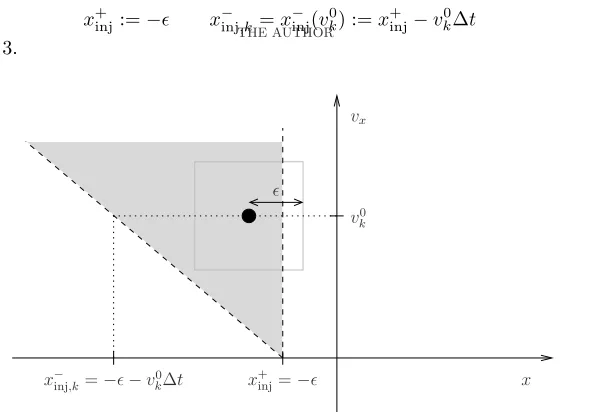
Finally, if we want to inject particles with different speeds the above procedure can be modified by adapting the length of the virtual loading region according to the actual velocity of each particle. Specifically, the random position of a particle loaded with velocityvx=v0k should be drawn on a virtual region [x
−
inj,k, x + inj]
corresponding to
x+inj:=− x−inj,k=x−inj(vk0) :=x+inj−v0k∆t (45) as depicted in Figure 3.
BRIEF ARTICLE
THE AUTHOR
ϵ
x x−
inj,k=−ϵ−vk0∆t x+inj=−ϵ
vx
v0
k
Figure 1. Your figure
1
Figure 3. Phase-space profile of the smooth particle injection. For a charge-conserving injection, particles must be loaded at each time step in a “virtual” region (outside the computational domainx≥0) where the inflow distributionfinjis extended uniformly with
respect tox < 0. For an accurate discretization with smooth shapes of radius , particles with an initial speed of vx = v0k must then be loaded following this virtually extended
distribution on an interval [−−vk0∆t,−].
3.3.
Numerical results
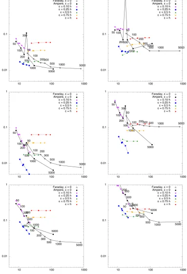
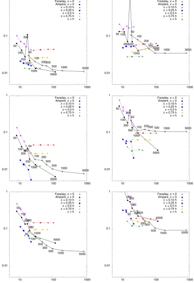
In Figures 4 and 5 we show the results obtained with the finite element scheme (13) coupled with the tensor-product Jacobs-Hesthaven particles (35) of degree 2a= 2 and 2a= 4 respectively, and we compare them with two standard mixed finite element schemes coupled with point particles. The key is as follows.
• All the curves display the relative error kFh−Frefk/kFrefk of some numerical fieldFh versus the
cpu time of the associated run. Here the considered fields are either the projected current density
Jh =π div,N I
the finite element magnetic field Bh (in the bottom rows), and the errors are measured inL2 (left
plots) andL∞(right plots).
• All the finite element schemes use the same mesh (an unstructured triangulation of the domain Ω = [0,0.1m]2 using 244 triangles with maximum diameterh
≈0.016 (m) and the same time range of about 1.6e−9 (seconds), chosen so that particles have travelled approximatively three diode lengths before the final time step where errors are measured. The time step ∆t has been computed from standard stability arguments for the leap-frog scheme. Its value is of about 4.5e−12, yielding about 360 time steps.
• The reference fields used to estimate the errors were obtained using a fine mesh of about 6000 triangles with maximum diameter h≈0.003, and about 250,000 smooth particles. Again the time step for these reference fields has been computed from standard stability arguments, its value is of about 9.1e−13, yielding about 1800 time steps. To validate their accuracy we have measured the distance (in L2 and L∞) between them and a sequence of solutions computed with meshes of
decreasing meshsize. These measures have allowed to estimate some upper bounds for the accuracy of the reference fields, and these bounds have been used as minimum values in the plotting ranges of the respective figures, so that every mark shown in Figures 4 and 5 is above those values. • Abscissas show the cpu times in seconds, each simulation being run on a 2.3 GHz Intel Core i7
laptop. Because depositing the current is the most expensive part, the runs were sped-up by a parallel treatment of the particles using 7 processes.
• Curves with dashed lines show results obtained with the “strong-Amp`ere” mixed finite-element method described (13) coupled with the smooth tensor-product particles (35). Each curve corre-sponds to a different ratio between the particle radius >0 and the mesh resolution h(defined as the maximum diameter of the triangles in the mesh), as indicated in the plots.
• Curves with solid lines show results obtained with point particles (= 0, that is S =δ) for com-parison, coupled with two different finite-element Maxwell solvers. The filled circles correspond to point particles coupled with the “strong-Amp`ere” finite-element scheme (13) and the empty cir-cles correspond to point particir-cles coupled with the standard “strong-Faraday” mixed finite-element scheme (17).
• In each curve, the different points correspond to different numbers Nppc of particles per cell. This
number determines the number of particles loaded in the virtual region outside the computational domain as described in Section 3.2. The value ofNppcis indicated in the point particles runs (where
it varies between 50 and 5000) but has been omitted for readibility in the smooth particle runs, where it varies between 5 and 50. Note that here the beam propagates on a region containing approximatively 90 triangular cells, so that in the steady-state regime the number of particles that are pushed at each time step in the computational domain is of about 90Nppc.
Observing first the convergence curves obtained with point particles (solid lines with circle points) we point out two facts.
• First, the “strong-Amp`ere” runs are much faster than the “strong-Faraday” ones. One reason for this is that in the latter runs one must solve at each time step a linear problem involving the mass matrix of the curl-conforming finite element space used for the electric field. In the “strong-Amp`ere” runs the linear problems to be solved involve the mass matrix of the continuous elements space for the magnetic field, which is much smaller sinceBis scalar valued. A second reason is that point particles deposit their current with less operations in the “strong-Amp`ere” scheme than in “strong-Faraday” schemes.
• Second, the Faraday” finite element scheme appears to be more robust than the “strong-Amp`ere” one, indeed with the latter we observe aberrant results for some values ofNppc. This may
be caused by the fact that when extended to point particles,πdiv h J
n+1/2
N is not a continuous function
of the particle positions. Indeed, when a particlekmoves exactly along a mesh edge this projection involves volume-based degrees of freedom ofJn+1/2k which are essentially products between a Dirac measure on an edge and a piecewise polynomial function that is fully discontinuous there. This effect does not appear when the particles deposit their current in the curl-conforming finite element space involved in the “strong-Faraday” scheme, as explained in [2, Lemma 3.1].
• Among the parameters for which different values are taken in our tests (i.e., the number of particles per cell Nppc, the ratio /h and the degree of the smooth particle shape), the most critical one
seems to be the ratio between the particle radiusand the maximum diameterhof the mesh cells. Specifically, our results indicate that the best results (in terms of accuracy and computational time) are obtained for smooth particles with radius in an approximate range of h/4 to h/2, and for particles shapes (35) with coordinate degree 2a= 4, the latter value seems to be the best choice for all the measured errors. Note that sincehis the maximumdiameterof the mesh cells, this amounts to taking smooth particles with approximatively the same diameter as the mesh cells.
• For the parameters chosen here, increasing the coordinate degree of the particles from 2a = 2 to 2a= 4 slightly improves the accuracy of the runs with particles radius of≥h/2 and it deteriorates those with≤h/4. It has no significant effect on the computational time.
• Increasing the numberNppc of particles per cell improves the numerical accuracy for small particles
(≤h/4) but has basically no impact for medium or large particles (≥h/2). On the other hand, it always deteriorates the cpu time of the runs.
• The best compromise between numerical accuracy and computational time seems to be obtained for smooth particles with coordinate degree of 2a= 4 and radius≈h/2 (i.e., particles with about the same diameter as the mesh cells), when usingNppc≈5−10 particles per cell. With those parameters
the computational time is about the same as when using the “strong-Amp`ere” finite element solver with about 200 point particles per cell, and the numerical accuracy is improved by a factor ranging from approximatively 2 (when measured inL2) to more than 4 (when measured inL∞).
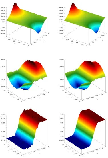
Finally, we show in Figure 6 the snapshots of the electro-magnetic fields corresponding to the “strong-Amp`ere” finite-element scheme coupled with about 200 point particles per cell (left plots) and about 5 smooth particles per cell (right plots), with the parameters described just above. As seen in Figure 5 these two runs took about the same cpu time (14 seconds), which clearly demonstrates the higher efficiency of the smooth particles for this test case.
Conclusion
In this work we have proposed a conforming finite-element scheme for the 2D time-dependent Maxwell sys-tem that preserves a strong Gauss law when the current is deposited from the particles with a Raviart-Thomas finite-element interpolation, and we have described an algorithm based on Fekete quadrature formulas for computing a numerical approximation of this current when the particles have a smooth shape. A numerical study involving an academic beam test-case with smooth injected current is used to assess the performances of the coupled scheme, and using a non-optimized implementation it is shown that with an appropriate choice of the particle parameters, the proposed method yields better results than two finite-element schemes coupled with point (Dirac) particles, for similar computation times.
References
[1] D. Boffi, F. Brezzi, and M. Fortin. Mixed finite element methods and applications, volume 44 of Springer Series in Computational Mathematics. Springer, 2013.
[2] M. Campos Pinto, S. Jund, S. Salmon, and E. Sonnendr¨ucker. Charge conserving FEM-PIC schemes on general grids.C.R. M´ecanique, 342(10-11):570–582, 2014.
[3] M. Campos Pinto and E. Sonnendr¨ucker. Gauss-compatible Galerkin schemes for time-dependent Maxwell equations. hhal-00969326i(to appear in Mathematics of Computation), 2014.
[4] V. Girault and P.-A. Raviart. Finite Element Methods for Navier-Stokes Equations – Theory and Algorithms. Springer Series in Computational Mathematics. Springer-Verlag, Berlin, 1986.
[5] J.S. Hesthaven. From Electrostatics to Almost Optimal Nodal Sets for Polynomial Interpolation in a Simplex. SIAM Journal on Numerical Analysis, 35(2):655–676, April 1998.
[6] G.B. Jacobs and J.S. Hesthaven. High-order nodal discontinuous Galerkin particle-in-cell method on unstructured grids.
Journal of Computational Physics, 214(1):96–121, May 2006.
[7] J. Loverich, C. Nieter, D. Smithe, S. Mahalingam, and P. Stoltz. Charge conserving emission from conformal boundaries in electromagnetic PIC simulations. Unpublished (2010),http://www.john-loverich.com/emission.pdf.
[8] P. Monk. A mixed method for approximating Maxwell’s equations.SIAM Journal on Numerical Analysis, pages 1610–1634, 1991.
[9] M.L. Stowell and D.A. White. Discretizing transient current densities in the Maxwell equations. In Proceedings of the ICAP 2009, 2009.
[10] M.A. Taylor, B.A. Wingate, and R.E. Vincent. An algorithm for computing Fekete points in the triangle.SIAM Journal on Numerical Analysis, 38(5):1707–1720, 2000.
Figure 4. Relative error curves vs. cpu times obtained with tensor-product Jacobs-Hesthaven particles of coordinate degree 2a= 2 and different values for the particle radius
>0. Filled and empty circles (black curves) correspond to simulations using point particles (= 0), see the text for details. Here the errors are measured inL2(left) andL∞(right) for
Figure 5. Relative error curves vs. cpu times obtained with tensor-product Jacobs-Hesthaven particles of coordinate degree 2a= 4 and different values for the particle radius
>0. Filled and empty circles (black curves) correspond to simulations using point particles (= 0), see the text for details. Here the errors are measured inL2(left) andL∞(right) for
Figure 6. Academic beam test-case. Snapshots of the self-consistent fields (Exon the top
row,Ey on the center row andB on the bottom row) obtained with the “strong-Amp`ere”
mixed finite-element scheme (13) coupled with point particles (left plots) and smooth Jacobs-Hesthaven particles (35) of radius = h/2 (right plots) with respective numbers Nppc of
![Figure 1. Example of a triangular mesh cellFigure 1. T Your figure (with its Fekete points for q = 3) intersectingthe convex support ΩS(k, n) of the k-th particle moving on the time step [tn, tn+1].](https://thumb-us.123doks.com/thumbv2/123dok_us/10064310.1992772/9.612.197.421.491.626/figure-example-triangular-cellfigure-fekete-intersectingthe-support-particle.webp)