Unsteady aerodynamics using high order methods

(1)

ePrints Soton

Copyright © and Moral Rights for this thesis are retained by the author and/or other

copyright owners. A copy can be downloaded for personal non-commercial

research or study, without prior permission or charge. This thesis cannot be

reproduced or quoted extensively from without first obtaining permission in writing

from the copyright holder/s. The content must not be changed in any way or sold

commercially in any format or medium without the formal permission of the

copyright holders.

When referring to this work, full bibliographic details including the author, title,

awarding institution and date of the thesis must be given e.g.

(2)

Unsteady Aerodynamics Using High-Order

Methods

By

Prithiraj Bissessur

Doctor of Philosophy

SCHOOL OF ENGINEERING SCIENCES

February 2007

(3)

(4)

FACULTY OF ENGINEERING SCHOOL OF ENGINEERING SCIENCES

Doctor of Philosophy

Unsteady Aerodynamics Using High-Order Methods

by Prithiraj Bissessur

Unsteady flows occur in many applications of engineering interest. One category of unsteady flows occur as self-sustaining oscillatory fluid motion, such as the flow over rectangular cavities. There has been a significant amount of research performed on this topic over the years, both experimentally and numerically. The unsteady flow over rectangular cavities is the case study in this research.

In this work, a generic numerical solver is developed and written to predict the near-field aero-dynamics of unsteady fluid motions at low Mach numbers. High order numerical schemes are employed to this effect. The Detached Eddy Simulation (DES) method is considered for the tur-bulence modelling part. At the start of this project, the combination of high order Computational Aeroacoustics (CAA) numerical schemes, non-reflecting boundary conditions and DES consti-tuted a state of the art approach to the simulation of unsteady compressible flow phenomena at low Mach numbers.

In the numerical study of 2D cavities, a number of cases with different length-to-depth (L/D) ratios were considered. Under the same flow conditions, the relation of the L/Dto the radiated sound in the farfield is sought. It is found that the nature of the flow interaction with the downstream corner, which changes withL/D, dictates the directivity and amplitude of the sound field observed at a far distance from the source.

To gain more insight into the topology of 3D cavity flows, an experimental study using non-intrusive measurement techniques is outlined. This explains the work performed on 3D cavities with different spanwise dimensions. A detailed flow visualisation of the meanflow patterns in various measurements planes describes the presence of strong 3D features. In particular, the sym-metrical flow behaviours at relatively large width-to-depth (W/D) ratios of 3 and 2 are highlighted. This provides the justification to employ a symmetry condition in the 3D DES study.

(5)

Acknowledgements

I am grateful to my supervisor, Professor Xin Zhang for his patience and invaluable guid-ance during the course of this project.

I would also like to thank Dr. Xiaoxian Chen, Dr. Graham Ashcroft and Dr. Kenji Takeda for their help and assistance during the early stages of the project. Their contribution to the high order flow solver described in this work is gratefully acknowledged.

To Simon, whom as my office mate had to endure my musical taste. Thanks to Ajay, Mahbs, Shu and Abdul for making my time in Southampton truly memorable.

Special thanks to Miss Sonya Davy for having accommodated me for three years. I am grateful for her friendship and support during the course of my project.

(6)

List of Tables

1.1 αfor variousL/D. . . 7

2.1 Stencil coefficients for the sixth-order forward and backward pre-factored compact operators. . . 31

2.2 Stencil coefficients for inter-block boundaries. . . 32

2.3 Biased stencil coefficients for the forward and backward operators. . . 32

2.4 Five-point stencil coefficients for the fourth-order optimized pre-factored scheme. . . 33

2.5 Biased stencil coefficients for the five-point fourth-order scheme. . . 34

2.6 LDDRK four/six stage scheme coefficients. . . 36

5.1 Mean re-circulation centre positions forW/D=3. . . 104

5.2 Mean re-circulation centre positions forW/D=2. . . 104

5.3 Mean re-circulation centre positions forW/D=1.5. . . 104

5.4 Mean re-circulation centre positions forW/D=1.0. . . 105

(13)

5.6 Mean re-circulation centre positions for 2D cavity. . . 105

(14)

List of Figures

1.1 Schematic of flow over a cavity. . . 19

1.2 Schematic of cavity flow feedback loop. . . 19

1.3 Schematic of flow over an open and transitional-open cavity and pressure distribution along the floor. . . 20

1.4 Schematic of flow over an closed and transitional-closed cavity and pres-sure distribution along the floor. . . 20

2.1 Laminar flat plate boundary layer. . . 41

2.2 Laminar flow over a flat plate, Mach 0.5. . . 42

2.3 Turbulent flat plate boundary layer. . . 43

2.4 Turbulent flat plate boundary layer computation. . . 44

3.1 Computational meshes employed for grid sensitivity study: (a) coarse mesh and (b) fine mesh. . . 50

3.2 Time variation of pressure fluctuations for the coarse and fine meshes: (a) pressure fluctuations and (b) spectra,∆St=0.0003. . . 51

(15)

3.4 Pressure variation along the cavity floor,y/D=-1.0. . . 52

3.5 Local Mach number variation alongy/D=₋0.9. . . 53

3.6 Time averaged streamline patterns: (a) coarse mesh and (b) fine mesh. . . 54

3.7 Time averaged vorticity contours: (a) coarse mesh and (b) fine mesh. . . . 55

4.1 2D cavity geometry. . . 74

4.2 Typical computational domain, with 574,000 cells. Flow from left to right. 74 4.3 Static pressure distribution along the cavity floor atM_∞=0.5. . . 75

4.4 Time-averaged streamline patterns;L/D=2, M∞=0.5. . . 75

4.6 Time-averaged streamline patterns;L/D=5, M_∞=0.5. . . 76

4.8 Time-averaged streamline patterns;L/D=10, M_∞=0.5. . . 77

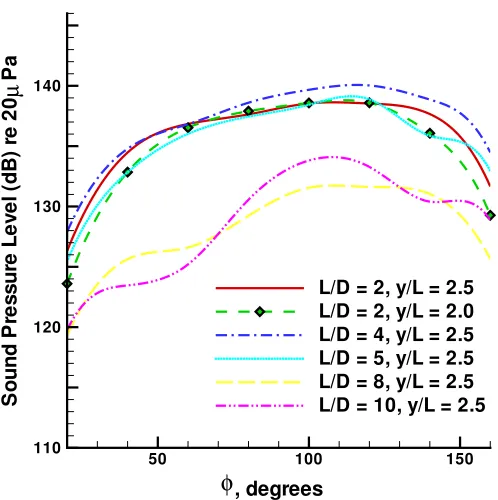
4.9 Sound Pressure Level in dB,L/D=2, x/L=0.5,∆St=0.0025. . . 78

4.10 Sound Pressure Level in dBL/D=4, x/L=0.5,∆St=0.0033. . . 78

(16)

4.15 Instantaneous non-dimensional vorticity Ω and dilatation (dashed lines)

Θ;L/D=4, M_∞=0.5. . . 82

4.16 Instantaneous non-dimensional vorticity Ω and dilatation (dashed lines) Θ;L/D=5, M_∞=0.5. . . 83

4.17 Instantaneous non-dimensional vorticity Ω and dilatation (dashed lines) Θ;L/D=8, M_∞=0.5. . . 84

4.18 Instantaneous non-dimensional vorticity Ω and dilatation (dashed lines) Θ;L/D=10, M∞=0.5. . . 85

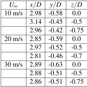
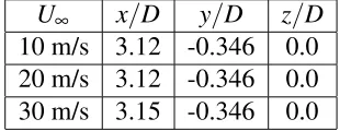
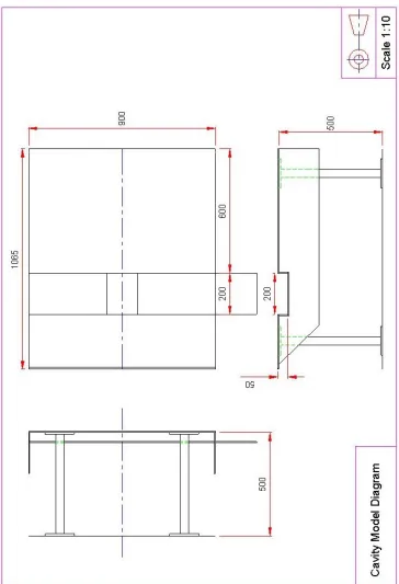
4.19 Far-field sound pressure level and directivity for varyingL/D;M_∞=0.5. 86 5.1 Cavity model drawing, all dimensions in mm. . . 106

5.2 2D cavity configuration. . . 107

5.3 3D cavity configuration. . . 107

5.4 Schematic of the model setup in the wind tunnel. . . 107

5.5 Unfolded view of surface flow visualization,W/D=3,U_∞=30m/s. . . . 108

5.6 Unfolded view of surface flow visualization,W/D=2,U∞=30m/s. . . . 109

5.7 Unfolded view of surface flow visualization,W/D=1.5,U_∞=30m/s. . 110

5.8 Unfolded view of surface flow visualization,W/D=1,U∞=30m/s. . . . 111

5.9 Unfolded view of surface flow visualization,W/D=0.5,U_∞=30m/s. . 112

(17)

5.11 Mean sectional streamlines at various spanwise positions,W/D=2,U_∞=

30m/s. . . 114

5.12 Mean sectional streamlines at various spanwise positions, W/D= 1.5,

U_∞=30m/s. . . 115

5.13 Mean sectional streamlines at various spanwise positions, W/D= 1.0,

U_∞=30m/s. . . 116

5.14 Comparison of 3DW/D= 0.5 cavity and 2DW/D= 18 cavity. Flow

from left to right. . . 117

5.15 Comparison of surface oil flow against PIV data,W/D=3, y/D=-0.9;

U∞=30 m/s. . . 118

U∞=30 m/s. . . 119

5.17 Comparison of surface oil flow against PIV data,W/D=1.5,y/D=-0.9;

U∞=30 m/s. . . 120

U_∞=30 m/s. . . 121

5.19 Comparison of surface oil flow against PIV data,W/D=0.5,y/D=-0.9;

U_∞=30 m/s. . . 121

5.20 LES decomposition with Galilean transformation (2D,W/D=18, U∞=

30m/s), Flow from Left to Right. . . 122

5.21 LES decomposition with Galilean transformation of the shear layer (3D,W/D=

3,U_∞=30m/s). . . 123

5.22 LES decomposition with Galilean transformation at the trailing edge (3D,W/D=

(18)

5.23 LES decomposition with Galilean transformation of the shear layer (3D,W/D=

1,U_∞=30m/s). . . 125

5.24 LES decomposition with Galilean transformation at the trailing edge (3D,W/D=

1,U_∞=30m/s). . . 126

6.1 3D cavity geometry. . . 138

6.2 Time averaged sectional streamlines across the cavity span, flow from left to right. . . 139

6.3 Static pressure distribution along the cavity floor at different spanwise locations. . . 140

6.4 Flow pattern along the cavity floor, flow from left to right. . . 141

6.5 Flow visualization along the cavity floor and vertical plane corresponding

toz/D=0.95. . . 142

6.6 Sound Pressure Level in dB,L/D=2,W/D=2,x/D=1.0,∆St=0.0012.143

6.7 Q-criterion visualization describing three-dimensional cavity time-dependent

flow ;M_∞=0.4. . . 144

6.8 Instantaneous density fluctuation (ρ/ρ_∞₋1): x₋yplane,z/D=0.0. . . . 145

6.9 Instantaneous density fluctuation (ρ/ρ∞−1): x−zplane,y/D=0.2. . . . 145

6.10 Instantaneous density fluctuation (ρ/ρ_∞₋1): y₋zplane,x/D=1.0. . . . 146

6.11 Acoustic field directivity at 100L in thex₋yplane aboutz/D=0.0. . . . 147

(19)

Nomenclature

a Speed of sound

Cp Pressure coefficient,(p−p∞)/1₂ρ∞U∞2

cp Specific heat coefficient at constant pressure

cv Specific heat coefficient at constant volume

e Specific internal energy

et Specific total energy

f Frequency

G Generic Green’s function

G0 Free space Green’s function

H() Heaviside function

J Jacobian

k Specific turbulent kinetic energy

M Mach number

p Static pressure

Pr Prandtl number

PrT Turbulent Prandtl number

qx,qy,qz Heat flux in Cartesian coordinate system

(20)

Re Reynolds number

St Strouhal number

t Time

T Temperature, unless otherwise stated

Ti j Lighthill stress tensor

u,v,w Cartesian coordinate velocity components

ui Cartesian velocity components (u1,u2,u3)≡(u,v,w)

U,V,W Contravariant velocity components

L Cavity length

D Cavity depth

W Cavity width or span

v Velocity vector

Greek Symbols:

α Phase lag in the Rossiter equation

ρ Fluid density

δ Boundary layer thickness

δi j Kronecker delta function

δ() Dirac delta function

δ∗ _{Displacement thickness}

µ Fluid molecular viscosity

ν Kinematic viscosity,ν=µ/ρ

τw Wall shear stress

τi j Viscous stress tensor

ξ,η,ζ Orthogonal curvilinear coordinate

φ Generic field notation

(21)

κ Wavenumber

κx,κy,κz Directional wavenumbers in Cartesian space

σi Root-mean-square of the velocity fluctuationu0_i

Π LES filter function

∆ Filter width

Superscripts:

() Time averaged quantity

e

() Favre averaged quantity

()∗ Dimensional quantity

()0 Fluctuation quantity

() Filtered quantity

Subscripts:

()0 Reference quantity

()_∞ Free stream quantity

()t Total stagnation condition

()T Turbulent quantity

(22)

<> Time averaged quantity

Abbreviations:

CAA Computational AeroAcoustics

CFD Computational Fluid Dynamics

CFL Courant-Friedrichs-Levy criterion (or Courant number)

DFT Discrete Fourier Transform

DRP Dispersion Relation Preserving

SPL Sound Pressure Level, decibels (dB)

MPI Message Passing Interface

FW-H Ffwocs Williams and Hawkings

FFT Fast Fourier Transform

PIV Particle Image Velocimetry

POD Proper Orthogonal Decomposition

DNS Direct Numerical Simulation

DES Detached Eddy Simulation

LES Large Eddy Simulation

RANS Reynolds Averaged Navier-Stokes

CCD Charged Coupled Device

2D Two-dimensional

3D Three-dimensional

RK Runge-Kutta

LDDRK Low Dispersion and Dissipation Runge-Kutta

(23)

Chapter 1 Introduction

1.1 Motivation

Cavity noise appears in large number of applications where a cutout of some description is subjected to an oncoming flow. When the conditions are right, self-sustained oscillations can occur inside the cavity where undesirable effects such as vibrations (fluid-structure interaction), noise generation, increase in drag and a change in the thermal transfer char-acteristics can arise.

The presence of a cavity creates large fluctuations in pressure, density or velocity, thereby giving rise to an intense acoustic radiation. The first experimental investigations into

cavity flows were in the years 1950−1960 [1, 2]. These were primarily dedicated to

military aircraft with bomb bays, which, when open resembled rectangular cavities. The cavities thus studied were of large physical dimension and the flow speeds were in the high

subsonic or supersonic regimes. In the 19700_s _{there was an apparent need to consider}

lower flow speeds where it was identified that aircraft landing gear wheel wells during take-off and landing were similar, in generic terms, to rectangular cavities [2, 3].

(24)

reso-nant systems such as the multi-stage compressor arrangement in the combustion chamber of jet engines. The resonance mechanism here is a function of geometric parameters and can be classed as a Helmholtz resonator [4, 5].

In non-aeronautical applications, cavities are also present, i.e. rail wagons (where the gap between carriages form a rather large cavity) and door cavities in the automobile appli-cations. The aeroacoustic oscillations created in such applications can be a significant detriment to the comfort of passengers as well as a nuisance to the surrounding environ-ment. The variety of applications and the complexity of the phenomena involved have inspired quite a number of experimental, theoretical and more recently computational investigation into cavity flow physics. Most research tends to focus on the flow charac-teristics and acoustics. However, recently a new trend has been set into devising methods for the active or passive control of cavity noise [6, 7, 8]. In the following sections, the terminologies associated with cavity flows are explained and the relevant experimental, theoretical and computational work over the years is reviewed.

1.2 Cavity Terminology

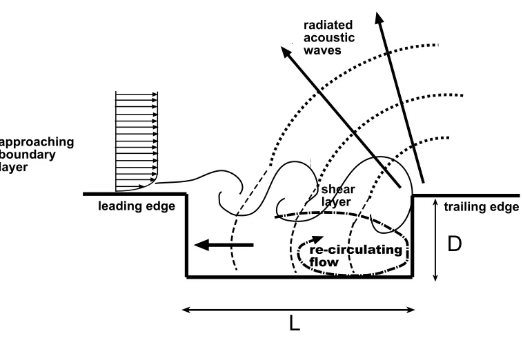
A generic rectangular cavity can be characterised by its length L, depthD and spanW.

These notations are shown in Figure 1.1, where a 2D cavity is represented. While the geometry is simple as shown in Figure 1.1, the underlying physics of the flow over such arrangements is complex. Cavity flows have been observed to exhibit flow phenomena rich in unsteady fluid dynamics, flow-acoustic interaction and flow-acoustic resonance. It is no trivial task to classify the flow regimes that can be observed over cavities. The

important parameters that can influence the flow regime observed are the inflow speedU_∞,

the incoming boundary layer momentum thicknessθ, the ambient fluid parameters such

as the air densityρ∞, the ambient speed of sounda∞and the basic geometric parameters

of the cavity,L,DandW.

(25)

param-eters. The ratios length to the depth and the length to width of the cavity are therefore

critical. Roshko [9] observed that the L/D has a strong influence over the nature of the

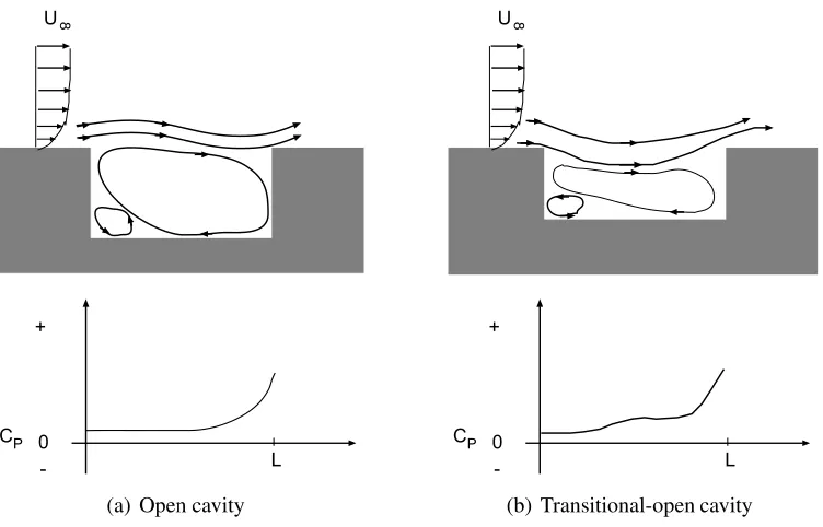
flow. Four basic types of cavity flow regimes observed in experimental studies [10, 11] are the open, closed, transitional-open and transitional closed. In the open flow regime as shown in Figure 1.3(a), the shear layer across the cavity opening bridges the leading and trailing edge corners. The flow is dominated by a main large-scale re-circulating structure within the cavity. The static pressure distribution is characterised by a single minimum corresponding to the centre of the flow recirculation. This type of flow regime is generally

observed for cavities ofL/D_≤6 up to a maximum ofL/D_≤8 at subsonic and transonic

speeds. The second type of cavity flow is the closed flow regime which concerns cavities termed as ‘shallow’. This characteristics of this flow regime is shown in Figure 1.4(a). In this case the shear layer re-attaches somewhere along the cavity floor and separates again as the flow passes the trailing edge corner. Two distinct re-circulating zones are observed, one upstream and the other downstream of the re-attachment and separation zone on the cavity floor. The static pressure along the cavity floor in this case is characterised by a strong adverse pressure gradient as shown in Figure 1.4(a). The occurrence of this flow regime is largely influenced by the flow Mach number. For subsonic and transonic speeds,

this flow regime can be observed forL/Dvalues between 9 and 15. At supersonic speeds,

the closed flow regime is observed for L/D_≥ 13. The flow regime that falls between

open and closed is termed transitional. Figure 1.3(b) shows the characteristic transitional-open cavity flow. The static pressure distribution along the floor is mainly uniform in the forward portion but increases towards the aft portion of the cavity. The fourth cavity flow regime is the transitional-closed flow shown in Figure 1.4(b). In this case, the static pressure experiences a continuous increase over most of the floor. Another important

ge-ometrical parameter is the ratio of length-to-width which defines 3D cavities. ForL/W _≤

1, the shear layer has been found to exhibit more or less a 2D behaviour, whereas for

L/W > 1, three dimensional effects come into play as shown by Maull and East [12].

Thus for relatively shallow cavities ofL/D_≥4 andL/W >1, 3D effects were observed

(26)

The type of flow regime largely influences the nature of the unsteady flow in and around the cavity. Closed cavity flows often display broadband pressure fluctuations whereas open cavity flows are typified by highly periodic flow phenomena. To determine the

influence of the cavity depth on the flow characteristics one must consider the ratioD/δ0,

whereδ0is the thickness of the oncoming boundary layer. Below a certain value ofD/δ0

the frequency of the oscillations is minimised. On the other hand, as shown by Kuo et

al [13], the re-circulation region inside the cavity can modulate the path and behaviour

of the shear layer. The transition from an open cavity to a closed cavity depends on the flow Mach number as shown by Tracy and Plentovich [14]. Sarohia [15] defined a

non-dimensional length, (L/δ0)pReδ0, where L is the length of the cavity and Reδ0 is the

Reynolds number based on the boundary layer thickness. For laminar flow over a cavity,

this non-dimensional length is independent of the normalised depthD/δ0forD/δ0≥2.

It is also found that if the non-dimensional minimum length is below a value of 0.29_×103

no cavity oscillation occurs [15].

The nature of the oscillations that may develop in an open cavity flow regime is dependent

on the value of L/D. For cavities where L/D are small, transverse standing waves are

present and the such cavities are classed as ‘deep’. For valuesL/Dwhich are sufficiently

large, longitudinal standing waves are observed and such cavities are termed as ‘shallow’.

Generally, cavities are classed as ‘deep’ when L/D<1 and classed as ‘shallow’ when

L/D> 1. Therefore, a second classification of the cavity flow problem is based on the

characteristics of the oscillations which occur. For this purpose, three distinct classes of interactions between the flow and the cavity have been identified:

• Dynamic (hydrodynamic or aerodynamic)

• Resonant (acoustic)

• Elastic (fluid-structure)

(27)

associated with the compressibility of the of the fluid (standing waves inside the cavity and Helmholtz type resonator). The elastic interaction is a fluid-structure interaction and has to do with the elastic deformation of solid surfaces. The current study is limited in scope to the dynamic and acoustic phenomena only.

1.3 Review of Experimental and Theoretical Work

The experimental work of Roshko [9] and that of Karamcheti [16] in 1955 constituted the first substantial investigation into cavity flow physics and the subsequent noise ra-diation. In particular, Roshko highlighted the importance of the geometrical parameters on the meanflow. For shallow cavities at low Mach numbers, a main vortical region with secondary re-circulating regions in the corner (Moffatt eddies) is observed. The main con-clusion from this study is that the drag on the cavity is directly related to the stagnation pressure occurring on the downstream wall when the shear layer impinges on it.

On the other hand, the work carried out by Karamcheti was the first attempt to consider the radiated noise and remains to this day as one of the rare references where the influence of the meanflow on the sound field is clearly illustrated. It was noted that the directivity of the radiation was towards the leading edge for high Mach numbers. The primary reason for this is due to the convection of the acoustic waves by the meanflow. In his study, the influence of the nature (laminar or turbulent) of the oncoming boundary layer was also investigated. It was observed that the peaks in the spectra of the pressure fluctuations were more intense when the incident boundary layer was laminar and more broadband for a turbulent one.

Plumbleeet al[17] investigated the acoustic resonance phenomenon. The authors showed

(28)

mech-anism of the acoustic modes related to the cavity geometry. However, this observation contradicts the observation that for the laminar case, the acoustic field is more intense.

In 1963, Maull and East [12], performed an experimental investigation to demonstrate the 3D nature of the flow inside the cavity. Cellular re-circulating structures were observed

for certain spanwise length W of the cavity. The existence of these structures and an

odd or even number of cells is directly related to the size of the primary vortex in the streamwise direction. The cellular structures are visible at low speeds but can also appear at high speeds. It was concluded that 3D effects can also play an important of role on the oscillations and hence the acoustic field.

In 1964, Rossiter [18] studied cavity flows in the L/D range from 1 to 10 and at Mach

numbers ranging from 0.4 to 1.2. This study provided the first satisfactory explanation of the aerodynamic coupling that produces self-sustained oscillations. It was concluded that the periodic pressure fluctuations might be attributed to an acoustic resonance within the cavity and is very similar to the ‘edge-tone’ excitation. Rossiter observed large-scale

vortical structures in the shear layer that span the cavity opening. For a cavity of lengthL,

the convection velocity of the large scale vortical structure isUcand thus the convective

time scale isL/Uc. In a free shear layer, the convection speed is anywhere between 0.4Uc

to 0.6Uc. With this information, a plot of Strouhal number(St= f L/U∞), where f is the

periodic shedding frequency, against Mach number (M) gives a direct empirical formula

which relatesSt,Mandn(the integer number of large scale vortical structures in the shear

layer). When a vortex impinges on the aft cavity wall, acoustic waves are generated and

propagate upstream of the cavity and reach the leading edge in timeL/a0, wherea0is the

speed of sound inside the enclosure which, at low Mach numbers, can be assumed equal

to the freestream sound speeda_∞. The amplitude of the periodic shedding gets amplified

by this process.

n

f =

L

Uc+

L

(29)

L/D α

4 0.25

6 0.38

8 0.54

10 0.58

Table 1.1:αfor variousL/D.

Rearranging equation (1.1) gives

St= f L

U∞ =

n U∞

Uc +M∞

(1.2)

When the impingement of the vortical structure occurs, there is a phase lag between the the emission of acoustic waves. Similarly, there is a phase lag between the arrival of a pressure wave at the leading edge and the roll-up of a new vortex. Thus equation (1.2) is re-written as,

St= f L

U_∞ =

n₋α

1

κ+M∞

(1.3)

Whereαis the phase lag andκis the ratio of the freestream velocity to the mean

convec-tion velocity. Usually, αis taken as 0.25. Table 1.1 gives values ofαfor a range ofL/D

from 4 to 10.

Although the Rossiter formula, equation (1.3), is a popular model for predicting cavity oscillations, it does not take into account the characteristics of the oncoming boundary

layer, the acoustic resonance modes and the influence of the cavity depthD, all of which

can significantly modify the properties of the flow if self-sustained oscillations occur and implicitly infers that the feedback mechanism is of an acoustic nature.

(30)

as described by Plumblee et al [17]. At high Mach numbers, the aeroacoustic feedback predominates and the Rossiter formula is applicable but at low Mach numbers, the two mechanisms co-exist. When the fundamental frequencies of the acoustic modes and the oscillation modes coincide, a double resonance effect is produced that amplifies the am-plitude of the shear layer oscillation.

Helleret al[20] accounted for the local variation of the speed of sound in the cavity and

extended the Rossiter results to high Mach numbers above Mach 1.2. At such speeds, the speed of sound inside the cavity can no longer be taken as equal to the freestream value but is determined by the local static temperature, thus

acavity

a∞ =

r

1+rγ−1

2 M2∞ (1.4)

whereris the thermal recovery factor

r= Tc−T∞

T0−T∞ (1.5)

where Tc is the temperature in the cavity and T0 is the stagnation temperature. At high

Mach numbers,r_'1. Substituting equation (1.4) into the Rossiter formula (1.3) gives,

St= f L

U_∞ =

n₋α

1

κ+q₁₊M_rγ∞−1 2 M2∞

(1.6)

(31)

parameters such as L/Dand the non dimensional length as defined by Sarohia [15] en-abled them to improve on the Bilanin and Covert model. The Tam and Block model takes into account the aeroacoustic coupling but cannot predict the acoustic depth modes that occur at low speeds.

On the other hand, Heller and Bliss [23] consider the fluid injection and ejection at the trailing edge corner of the cavity as the primary effect to the resulting oscillations. In their study, the downstream edge was substituted by a pseudo-piston. The mass addition and removal creates pressure fluctuations that travel upstream in the cavity and thereby further amplify the vortices that are shed at the leading corner. In this manner the cavity acoustic wave generated is coupled with the motion of the shear layer and thus completing the feedback loop.

In 1987, Gharib and Roshko [24] conducted an experimental investigation into an ax-isymmetric cavity flow where the transition of the shear layer oscillation modes to a new regime was found. Under the condition that the oncoming boundary layer was thin, the shear layer resembled the wake pattern behind a bluff body. This regime was appro-priately termed a ‘wake-mode’ type oscillation. In this case the cavity flow undergoes alternating filling and emptying phases in a manner that is indicative of an absolute

in-stability as shown by Theofilis et al [25]. This gives a large increase in the drag of the

cavity and is mainly observed for shallow cavities. Deep cavities tend to behave in a more quiescent fashion and this type of oscillation is termed the ‘shear-layer’ mode regime, i.e. the Rossiter modes.

In a series of experiments by Plentovich [26, 11] and Tracy and Plentovich [14, 27], detailed static pressure data have been compiled for 3D cavities at subsonic and transonic

speeds and high Reynolds numbers in order to characterise the flow field. The cavityL/D

ratio ranges from 4.4 to 20.0 in the experiments andW/Dbetween 1.0 and 4.5. A wide

range of flow speeds have been investigated, and the flow Reynolds number varied from

1.0_×106to 1.0_×108. Both static coefficients of pressure as well as the fluctuating sound

(32)

In 1996, Ahuja and Mendoza [28] delivered a comprehensive database on the influence

of various parameters such as L/D, L/W, the oncoming boundary layer properties and

temperature effects on the oscillations occurring in the cavity. This study is one of the rare cases where there is an attempt to relate the far-field directivity to the near-field flow physics (near-field pressure fluctuations). Also, to characterise the 3D effects, the authors

studied the effect of varying the cavity spanW. ForL/W<1, the behaviour of the radiated

noise was found to be that of a 2D cavity.

Particle Image Velocimetry (PIV) investigations enabled the near-instantaneous velocity field of cavity flows to be recorded. PIV measurements of the turbulent flow over a cavity

were carried out by Lin and Rockwell [29]. Kuoet al [13] recently used the same

tech-nique to study the effect of modifying the base of the cavity (i.e. replacing the floor with a slope) on the flow.

1.4 Dynamic Oscillations and the Feedback Mechanism

Since the edge-tone phenomenon was observed by Sondhaus in 1854, self-sustained os-cillations have been noted for a large number of flows where the shear layer strikes an obstacle. Rockwell and Naudascher [30] have compiled a comprehensive collection from the literature on these types of flows.

Self-sustained oscillations occur in the presence of a chain of events that are the necessary conditions for the flow instability to self-sustain,

• The feedback process takes place when perturbations at the cavity trailing edge due

to the impingement of the large scale vortical structures are propagated upstream to the leading edge corner. This region of the flow is particularly sensitive to distur-bances as the boundary layer separates there (receptivity process).

(33)

• These perturbations convectively amplify across the cavity mouth.

• New perturbations at the downstream cavity edge are formed by the impingement

of the shear layer fluctuations against the solid boundary. These perturbations travel upstream thus closing the feedback loop.

Experimental investigations into cavity flows under varying conditions have shown that the disturbances that propagate upstream are either acoustic or aerodynamic in nature.

At high speeds, when the characteristic acoustic wavelength λ is of the same order as

the length scale, L, it is important to take into account the speed of sound to determine

the retarded time between the impact zone and the separation zone. Powell [31] showed that there is an acoustic radiation towards the upstream region and suggested that simple acoustic sources be used to model the acoustic feedback. For flows at very low Mach numbers, the feedback process is instantaneous and occurs in the vicinity of the acoustic source. The feedback process is essentially of an aerodynamic nature. However, there is always an influence of the coherent vortical structures on the upstream flow. This has also been observed in flow without obstacles at both low and high Mach numbers. The ques-tion thus arising is to what extent an obstacle modifies the arrangement of the coherent structures of the flow to lead to a feedback process. In the cavity case, the distribution of coherent structures is of a deterministic nature due to the fact that there is more or less a constant phase lag between the shedding of a new vortex and the impingement of another on the aft wall.

It is useful to examine the cavity feedback process using elementary control theory. With

reference to Figure 1.2, let ui(s) be the random fluctuation of the oncoming boundary

layer at the cavity leading edge. This fluctuation is selectively amplified with convection in the shear layer, so that at the downstream cavity edge the fluctuation has grown into

uo(s). This process is represented by H(s)in Figure 1.2. The impingement of uo(s)on

the downstream cavity edge creates a feedback pressure p(s)that travels upstream. The

generation of the pressure wave is represented by p(s)in Figure 1.2. As the pressure wave

(34)

layer receptivityR(s). The disturbanceu_d(s)adds to anyui(s)thus closing the feedback loop.

As identified by Rossiter [18], the necessary condition for a limit cycle to self-sustain is

that H(s) x p(s) x R(s) =1. Recently Rowley et al [32] suggested that certain cavity

flow oscillations occur not as self-sustained instabilities but as lightly damped

oscilla-tions. These require a constant inputui(s)from the turbulent structures in the oncoming

boundary layer.

1.4.1 Vorticity fluctuations

The conversion of pressure fluctuations reaching the separation point into vorticity has been studied by Morkovin and Paranjape [33]. It was found that the transverse pressure gradient plays an important role in this conversion process (receptivity). Moreover, the authors suggested that the periodic motion of the disturbances enables the conversion of an essentially irrotational disturbance field (pressure fluctuations) to a rotational distur-bance field (vorticity fluctuations). Linear stability analysis of nearly parallel flows can thus be adapted to account for the thickening of the shear layer. The frequency of the self-sustained oscillations lies in the region where the growth rate of these disturbances across the mouth of the cavity is positive.

1.4.2 Creation of disturbances at the aft corner

Where the large scale vortical structures impinge on the rear cavity edge, their defor-mation creates fluctuating forces on the downstream edge. Rockwell and Knisely [34] identified three ways in which these structures strike the trailing edge wall:

• Complete destruction, where there is a total breakdown of the large eddies.

(35)

spill inwards and outwards.

• The large scale vortices simply go around the corner and out of the cavity

For thin and turbulent oncoming boundary layers, none of these three types of deformation is predominant and there is more or less a random combination of these events. These are probably at the source of high and low frequencies in the sound power spectrum. The main re-circulation region can also modify the shear layer trajectory and determine where

it strikes the aft wall, as shown by Kuoet al[13]. This effect is neglected in all the models

relating to cavity flow oscillations and could potentially explain the variable way in which the shear layer interacts with the aft wall. All three types of deformation mentioned can be the source of the pressure fluctuations that subsequently travel upstream to further excite the shear layer and self-sustain the cavity flow instability.

1.5 Review of Computational Work

The first Computational Fluid Dynamics (CFD) simulations on cavity flows were per-formed by Hankey and Shang [35]. They used the Cebeci-Smith RANS model with the

McCormack scheme on a 2D cavity of L/D=2.25 at Mach 1.5. The simulations

com-pared favourably to the observations by Heller and Bliss [23]. Cavity flow simulations using RANS methods became popular in the 1990’s and were mostly validated with

sur-face pressure distributions around the cavity walls. Tam et al [36] studied the influence

of the turbulence models and showed that the results were sensitive to the model used

due to inherent dissipative nature of most models. This was confirmed by Slimon et

al [37]. The predictive ability of the RANS approach on a self-sustained cavity flow

(36)

The first 3D computations were performed by Rizetta [38] using an unsteady RANS ap-proach with the Baldwin-Lomax turbulence model. The advantage of RANS turbulence closure methods is that they are relatively easy to add to most CFD codes and provide a means to study the effect of varying the cavity geometry on the flow behaviour (passive control). Kim [39] replaced the cavity floor by a porous wall and obtained the same trends as observed in the corresponding experiments. Baysal [40] replaced the trailing edge

cor-ner by a ramp and Zhanget al[41] modified the geometry at the leading edge. Sinhaet al

[42, 43] used thek₋εmodel and a one equations Large Eddy Simulation (LES) approach

with wall functions to perform 3D unsteady simulations. Soemarwoto et al [44] used a

k₋ω turbulence model to compute the flow over a 3D cavity of L/D= 4.5 at a Mach

number of 1.2. The aim was to study the effect of replacing the trailing edge corner by a 45 degree ramp.

Direct Numerical Simulations (DNS) of cavity flows have also been tackled, for instance the calculation performed by Kestens [45] at low Reynolds numbers on 2D cavities for the study of open or closed flow oscillation control. A 3D simulation on a deep cavity of

L/D=0.42 andL/W =2 at a Mach number of 0.8 was performed by Sagaut [46]. This

simulation was at a low Reynolds number but was adequate to show 3D effects.

1.5.1 Supersonic simulations

The acoustic radiation arising from the supersonic flow over a cavity consists of a family of unsteady shock waves as described by Heller and Delfs [47]. Given the intensity of the shock waves, a conventional second-order accurate CFD simulation is sufficient to obtain the radiated pressure field. Moreover, these pressure waves cannot travel upstream of the flow. Numerous compressible unsteady RANS simulations have given a radiated

sound field as those visualised experimentally. For example, Zhanget al [48, 49, 50, 51]

have used an unsteady RANS method with a modifiedk₋ω model to take into account

(37)

laminar 2D cavity (L/D= 3) flow at Mach 1.5. In an attempt to investigate the cavity

flow instability, the authors concluded that the dominant cavity oscillation mode, which characterises the flow instability, is of a flow-resonant nature. In another study, Rona and Brooksbank [53] performed a POD analysis of the turbulent flow over a 2D cavity of

L/D=3 at Mach 1.5. In this study a simple low order model representing the cavity flow

instability was developed. The control of such flow instabilities was thus studied numer-ically by Rona [54]. In this study, blowing was applied at the cavity leading edge. The unsteadiness of the pressure field was reduced and subsequently disrupted the formation of the feedback loop.

1.5.2 Subsonic simulations

The first 2D laminar simulations in the subsonic regime leading to the radiated acoustic field were performed by Colonius [55] and Shieh and Morris [56] in 1999 for Reynolds

numbers based on the depth D (ReD ' 5000). These are in effect DNS computations

(no turbulence model) using Computational Aeroacoustics (CAA) algorithms and

non-reflecting boundary conditions. In the study by Coloniuset al[57, 55], a transition in the

flow regime is depicted, notably, there is a change from the classical Rossiter oscillation modes (shear layer mode) to the wake mode regime. This confirmed the observations by Gharib and Roshko [24] for shallow cavities with thin oncoming boundary layers. Shieh and Morris [58] applied the developments in CAA to the unsteady RANS methodology for

high Reynolds (ReD'10×105) number simulations. In this study the Spalart-Allmaras

one-equation turbulence model was hybridised to give a coupled RANS/LES technique called Detached Eddy Simulation (DES) for accurately resolving the separation regions in the flow. The transition from the shear layer mode to the wake mode is still observed.

Ashcroftet al[59, 60] used and unsteady RANS method with thek₋ωmodel for a door

cavity problem and the results were in good agreement with the measurements taken by Henderson [61].

(38)

various geometries. In shallow cavities, the transition to the wake mode is still observed

and in the highly 3D case (L/W >1), the oscillations were observed to be quite random

thus showing that the coherence of the self-sustained oscillations is somewhat affected in

the 3D case. For cavities of larger spanW, the self-sustained oscillations had a nearly 2D

behaviour.

The LES computation for the compressible flow over a deep cavity was performed by

Larchevˆeque et al [63]. An accurate prediction of the peak levels of the fundamental

frequency and its first harmonics was achieved relative to the available experimental data.

In another study by Larchevˆequeet al[64], the simulation of the flow over weapons bays

was performed. This study highlighted the existence of both transverse strong acoustic modes and vortical structures. The approach employed by these authors highlights a trend in the use of LES for the numerical simulation of flow over cavities.

1.6 Objectives and Scope of the Present Study

The present study is part of on-going research to further the current understanding into cavity flow oscillations. The aerodynamics of the flow is complex and, although quite a few theoretical and experimental as well as numerical studies have been performed, the analysis is yet to be completed.

(39)

reflections back into the computational domain. In addition to the computational work, wind tunnel testing using PIV was used to observe and record the flow patterns in 3D

cav-ities of varyingL/W. An experimental database was assembled that can be used for the

purpose of validating numerical work as well as to provide the cavity research community with a comprehensive set of data.

1.7 Structure of the Thesis

This thesis comprises of three parts. Part 1 spans Chapters 1 to 3 and constitutes the introductory chapters. In Chapter 1, a literature review is outlined. Chapter 2 provides an overview of the mathematical and numerical models employed in the present work. In Chapter 2 the governing equations are outlined and the numerical implementation is discussed both in terms of the spatial and temporal discretisation requirements. Boundary conditions, namely, non-reflecting buffer zone type inflow/outflow conditions are high-lighted. In Chapter 3, a mesh sensitivity study is performed on a 2D cavity case. This Chapter focuses mainly on the aerodynamic flow field and the results from two simula-tions are presented.

Part 2 focuses on 2D cavity flows and comprises of Chapter 4 alone. The aerodynamic

and acoustic field of 2D cavities of various L/D are examined. The results from the

simulations are presented separately for the aerodynamic and the acoustic analyses, where the latter is obtained from the FW-H integral method.

(40)

Part 3 examines 3D cavity flows using experimental and computational methods. This

analysis spans Chapters 5 and 6. In Chapter 5 low speed 3D cavity flows ofW/Dratios

(41)

1.8 Chapter 1 Figures

re-circulating flow

L

D

shear

layer approaching

boundary layer

leading edge trailing edge

radiated acoustic waves

Figure 1.1: Schematic of flow over a cavity.

H(s) +

R(s) p(s)

+

p(s)

u (s)_i

u (s)

d

[image:41.595.125.504.187.432.2]

u (s)_o

(42)

C_P +

-0 U8

L

(a) Open cavity

C_P +

-0 U8

L

[image:42.595.129.505.109.350.2]

(b) Transitional-open cavity

Figure 1.3: Schematic of flow over an open and transitional-open cavity and pressure distribution along the floor.

C_P +

-0 U8

L

(a) Closed cavity

C_P +

-0 U8

L

(b) Closed-transitional cavity

[image:42.595.131.504.429.680.2]

(43)

Chapter 2 Mathematical and Numerical Models

2.1 Introduction

This chapter describes the numerical methods employed in the current research. The choice of spatial and temporal discretisation will be described in details. Boundary con-ditions are especially important as the solution must not be allowed to be spoiled due to spurious reflections within the computational domain.

2.2 Modelling Approach

(44)

and Hawkings (FW-H) acoustic analogy [65, 66]. Since the work in this research did not involve the development of the FW-H solver, this chapter is limited to the description of the near-field methodology.

2.3 Governing Equations - Generalized Coordinate

Sys-tem

The flow variables (u,v,w,p,et) in equation (A.1) are given in terms of variations with

respect to a Cartesian frame of reference. To proceed to a numerical solution of the Navier-Stokes equations a set of orthogonal curviliear coordinates system is introduced,

represented as (ξ,η,ζ,t), corresponding to (x,y,z,t) respectively. This type of

representa-tion is usually referred to as body-fitted coordinates. This is a common practice in CFD when dealing with complex geometries. The governing equations (A.1) are recast to a rectangular uniform grid in the computational domain which is easier to handle when dealing with finite differences. The grid spacing in all directions is unity and the Jacobian of transformation relates the geometrical properties of the physical space to the computa-tional space.

ξ = ξ(x,y,z,t) (2.1)

η = η(x,y,z,t) (2.2)

(45)

The derivatives in (A.1) are transformed using the chain rule and it follows that:

∂ ∂x =

∂ ∂ξ _∂ξ ∂x + ∂ ∂η _∂η ∂x + ∂ ∂ζ _∂ζ ∂x ∂ ∂y =

∂ ∂ξ _∂ξ ∂y + ∂ ∂η _∂η ∂y + ∂ ∂ζ _∂ζ ∂y (2.4) ∂ ∂z =

∂ ∂ξ _∂ξ ∂z + ∂ ∂η _∂η ∂z + ∂ ∂ζ _∂ζ ∂z

The terms in brackets are called the metrics and relate the two coordinate systems. The metrics are derived from the general transformations given by equations (2.1) - (2.3). The time derivative remains unchanged for the fixed grid used in this study.

Substituting the transformed derivatives into equation (A.1) leads to the Navier-Stokes Equations for a curvilinear coordinate system, as shown below:

∂Q

∂t +

∂(F₋F_v)

∂ξ +

∂(G₋G_v)

∂η +

∂(H₋H_v)

∂ζ =0 (2.5)

where the solution vectorQand the flux vectors are given by:

Q=J

           ρ ρu ρv ρw

ρet           

,F=J

           ρu

ρUu+pξx

ρUv+pξy

ρUw+pξz

U(ρet+p)

          

,G=J

           ρV

ρVu+pηx

ρV v+pηy

ρV w+pηz

V(ρet+p)

          

,H=J

           ρW

ρWu+pζx

ρWv+pζy

ρW w+pζz

W(ρet+p)

           (2.6)

where (U,V,W) are the contravariant velocity components given by:

(46)

V =ηxu+ηyv+ηzw (2.8)

W =ζxu+ζyv+ζzw (2.9)

the viscous flux vectors are now defined as follows,

Fv=J

           0

ξxτxx+ξyτxy+ξz+τxz

ξxτxy+ξyτyy+ξz+τyz

ξxτxz+ξyτyz+ξz+τzz

ξxbx+ξyby+ξzbz            ,

Gv=J

           0

ηxτxx+ηyτxy+ηz+τxz

ηxτxy+ηyτyy+ηz+τyz

ηxτxz+ηyτyz+ηz+τzz

ηxbx+ηyby+ηzbz

           ,

Hv=J

           0

ζxτxx+ζyτxy+ζz+τxz

ζxτxy+ζyτyy+ζz+τyz

ζxτxz+ζyτyz+ζz+τzz

ζxbx+ζyby+ζzbz            , (2.10)

In equation (2.10), (bx,by,bz) are the viscous contributions to the heat flux arising in the

energy equation and these are expressed as

bx=uτxx+vτxy+wτxz+qx (2.11)

(47)

bz=uτxz+vτyz+wτzz+qz (2.13)

2.4 Turbulence Modelling: Spalart-Allmaras One

Equa-tion Model

For the purposes of modelling separated turbulent flows, the Spalart-Allmaras (S-A) one-equation turbulence model was implemented. The motivation behind the emphasis on the S-A model will become clearer in subsequent sections. Most one-equation models are based on the transport of turbulent kinetic energy. Nee and Kovasznay (1986), and more recently Baldwin and Barth (1990) and Spalart and Allmaras (1992) [67], have devised model equations for the transport of the turbulent viscosity (eddy viscosity) or a parame-ter proportional to the turbulent viscosity. The S-A turbulent kinematic viscosity is given by;

νT =ν˜fν1 (2.14)

The parameter ˜ν is an eddy viscosity that is obtained from the following transport

equa-tion:

∂ν˜

∂t +Uj

∂ν˜

∂xj =cb1 ˜

Sν˜₋cw1fw

_ν_˜ d

2 +1

σ ∂ ∂xk

(ν+ν˜) ν˜

∂xk

+cb2

σ ∂ν˜

∂xk

∂ν˜

∂xk (2.15)

The closure coefficients and auxiliary relations are;

c_b₁=0.1355, c_b₂=0.622, cv1=7.1, σ=2/3 (2.16)

(48)

fv1= χ 3

χ3₊_c3 v1

, fv2=1− χ

1+χfv1, fw=g

"

1+c6_w₃

g6₊_c6

w3

#1/6

(2.18)

χ= ν_ν˜, g=r+cw2

r6₋r, r= _˜ ν˜

Sκ2_d2 (2.19)

˜

S=S+_κ₂ν˜

d2fv2, Si j=

p

2Ωi jΩi j (2.20)

Ωi jis the rotation tensor based on the mean velocity gradients, given by;

Ωi j= 1 2

_∂_u i

∂xj−

∂uj

∂xi

(2.21)

One important observation in the S-A one-equation model is thatdis the distance from the

closest surface and hence the presence of a solid wall is automatically detected. The model can also include a transition correction that introduces four additional closure coefficients and two more empirical functions. The source terms for the eddy viscosity depends on

the distance from the closest surface, d, as well as upon the gradient of ˜ν. Asd _→∞,

the model also predicts no decay of eddy viscosity in a uniform stream far from solid

boundaries. The model has been proved to be far superior than most k₋εmodels in the

simulation of separated flows. The S-A model is coupled to the RANS by

µT=ρνT (2.22)

(49)

contributions, namely the (eddy) turbulent and laminar parts i.e. (µ+µT). The coefficient

of the heat transfer terms is replaced by (µ/Pr+µT/PrT), where PrT is the turbulent

Prandtl number and is taken as 0.9.

2.4.1 RANS-LES hybridisation

The RANS approach tends to be the industry standard for the calculation of turbulent wall bounded flows as it permits the modelling of relatively high Reynolds number flows rele-vant to engineering applications. The RANS approach tends to give poor results for bluff body flows, where large-scale motion has an important impact on the spatial evolution of the mean flow field. On the other hand, DNS or LES are often too expensive to be applied to commercial CFD work. The Detached Eddy Simulation (DES) approach aims to deliver affordable predictions of separated flows at high Reynolds numbers relevant to engineering applications. It combines a the RANS approach in boundary layer regions with the LES approach in separated flow regions.

2.4.2 The Detached Eddy Simulation concept

Detached Eddy Simulation or DES is a concept introduced by Spalart et al [68] for the

(50)

For the RANS model, the S-A one equation was initially used [68, 69], although techni-cally there are no obstacles in implementing other turbulence models that function in a similar way to the S-A model. The main advantage of the S-A one-equation model is that it will automatically detect the presence of a wall, which is ideal when one is attempting a numerical solution of an external aerodynamic flow, such as that over a 3D wing. The

standard S-A one-equation model uses the distance to the closest wall,d, as a length scale.

The DES modification involves substituting ford everywhere in the equations by a new

length scale ˜d, which now depends on the grid spacing,

˜

d=min(d,CDES∆) (2.23)

∆is based on the largest dimensions of the grid spacing, i.e.,

∆=max(∆x,∆y,∆z) (2.24)

It is then a matter of calibratingCDES, the empirical model constant, which was proposed

as 0.65 in [68]. This value provided a₋5/3 power law for the turbulent energy spectrum.

2.4.3 The motivation behind DES

RANS simulations have proven to be inaccurate to predict unsteady cavity flows. LES and DNS are too expensive to be used for complex geometries. Therefore for a full simulation of a turbulent boundary layer, the RANS method is the only choice available at present. This is the first response of a DES motivation, i.e. to render the computational costs more manageable and maintain a high level of accuracy, approaching that of DNS/LES.

For massively separated flows, RANS methods usually struggle to predict the onset of flow separation and the flow downstream of it. In this respect LES is an attractive option

to capture the large scale eddies (instabilities) accurately in a separated flow region. IfLis

(51)

the grid spacing must be of the order of `at most. As the energy carrying eddies have

`L, they can create a formidable task in terms of computational cost and number of

grid points required to resolve their motion. On the other hand, the characteristic length

scale of the turbulent structures in a boundary layer `2<δ<L, which is much smaller

than ell and thus would require an even finer computational mesh. In the solution for a

DES implementation, there are regions of ˜d_≈d, where the model functions in a RANS

mode, corresponding to a boundary layer type mesh, where, ∆d. Then in regions of

˜

d_≈CDES∆the model acts as a sub-grid scale for LES. These two regions are not explicitly

defined, as there is a single velocity and eddy-viscosity field. There have recently been various attempts to apply DES to different flow problems, for example, axi-symmetric jets as in [70], flow around a sphere [71], and cavity flow simulations [56].

2.5 Numerical Method

Aeroacoustics involves inherently unsteady phenomena over a wide spectrum of frequen-cies and amplitudes. To faithfully represent the sound source physics it is essential that the numerical algorithm captures all the relevant scales in the flow field. Hence the discreti-sation method (spatial and temporal) must have a low dispersion and dissipation errors so that the wave propagation characteristics are preserved. An appropriate spatial discretisa-tion can be obtained from a high order finite difference methods such as the one proposed by Lele [72]. In this work, a high-order compact finite-difference scheme similar to the one by Hixon [73] is used. The governing equations are integrated in time by a fourth or-der Runge-Kutta methods. Special non-reflecting boundary conditions are implemented that were developed specifically for CAA applications.

2.5.1 Spatial discretisation

(52)

achieve high-order accuracy by solving for the spatial derivatives as independent vari-ables at each grid point. The drawback with such methods is that the inversion of a matrix system is required at any point in the computational domain to compute the local spatial derivatives. Recently, Hixon [73] applied a pre-factorisation procedure to reduce the size of the computational stencil, thereby simplifying the boundary condition specification and enhancing its robustness. This procedure reduces the tri-diagonal matrix to a system of lower and upper bi-diagonal system that may be solved in parallel, thus increasing ef-ficiency. Recently Ashcroft and Zhang [74] further optimized the pre-factored schemes proposed by Hixon [73, 75] to obtain even smaller computational stencils and also im-prove the numerical wavenumber resolution characteristics of the scheme. According to

Lele [72], a general compact approximation to the first-order derivative (∂f/∂x) is given

by

βDi−2+αDi−1+Di+αDi+1+βDi+2=c

fi+3−fi−3

6∆x +b

fi+2−fi−2

4∆x +a

fi+1−fi−1

6∆x

(2.25)

whereDi is the spatial derivative of f at pointi. In the pre-factorisation as presented by

Hixon [73] the derivative ofDat a pointiis defined as being half the sum of the forward

and the backward derivatives

Di= 1

2(DFi +DBi) (2.26)

where DF

i is the forward derivative andDBi is the backward derivative. By defining the

forward and backward derivative operators using equation (2.25), the generic stencils for the forward and backward derivative operators for a sixth-order is

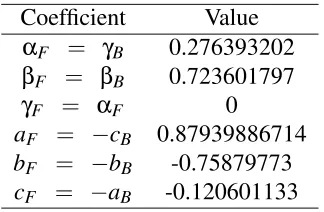
αFDFi+1+βFDFi +γFDFi−1= 1

∆x[aFfi+1+bFfi+cFfi−1] (2.27)

αBDB_i₊₁+βBD_iB+γBDB_i₋₁= _∆1

x[aBfi+1+bBfi+cBfi−1] (2.28)

(53)

orig-Coefficient Value

αF = γB 0.276393202

βF = βB 0.723601797

γF = αF 0

aF = −cB 0.87939886714

bF = −bB -0.75879773

[image:53.595.233.395.86.192.2]

cF = −aB -0.120601133

Table 2.1: Stencil coefficients for the sixth-order forward and backward pre-factored compact operators.

inal sixth-order central compact difference scheme is recovered. Using Fourier analysis as shown by Hixon and Turkel [75], it is possible to determine the coefficients of the scheme according to the required level of accuracy. In the present work, a sixth-order accurate scheme is chosen and the coefficients are given in Table 2.1.

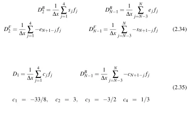
The central stencil presented in equations (2.27-2.28) are suitable only for the interior points of the computational space. If a multi-block approach is employed to subdivide the computational domain, at internal block boundaries, two eleven-point symmetric bound-ary stencils are employed. This stencil requires data from adjacent blocks. Thus the inter-block boundary stencil given by Hixon [76] is expressed as in equation (2.29). The corresponding stencil coefficients are given in Table 2.2. For other block boundaries, such as those at solid walls, two pairs of corresponding seven-point stencils are defined in equa-tion (2.30) for the forward and backward operators as developed by [73]. The one-sided stencil coefficients are given in Table 2.3.

DF_i = 1

∆x j=5

∑

j=−5

bifi+j DBi = _∆1_x

j=5

∑

j=−5−

bifi+j (2.29)

DF_i₌₁= 1

∆x 7

∑

j=1

−ejfi+j−1 DFi=N= _∆1_x N

∑

j=N−6

−sN+1−jfi+j−N

DB_i₌₁=_∆1

x 7

∑

j=1

sjfi+j−1 DBi=N=

1

∆x N

∑

j=N−6

Unsteady aerodynamics using high order methods

ePrints Soton

Copyright © and Moral Rights for this thesis are retained by the author and/or other

copyright owners. A copy can be downloaded for personal non-commercial

research or study, without prior permission or charge. This thesis cannot be

reproduced or quoted extensively from without first obtaining permission in writing

from the copyright holder/s. The content must not be changed in any way or sold

commercially in any format or medium without the formal permission of the

copyright holders.

When referring to this work, full bibliographic details including the author, title,

awarding institution and date of the thesis must be given e.g.

Unsteady Aerodynamics Using High-Order

Methods

By

Prithiraj Bissessur

Doctor of Philosophy

SCHOOL OF ENGINEERING SCIENCES

February 2007

Acknowledgements

Contents

List of Tables

List of Figures

Nomenclature

Greek Symbols:

Superscripts:

Subscripts:

Abbreviations:

Chapter 1

Introduction

1.1 Motivation

1.2 Cavity Terminology

1.3 Review of Experimental and Theoretical Work

1.4 Dynamic Oscillations and the Feedback Mechanism

1.4.1 Vorticity fluctuations

1.4.2 Creation of disturbances at the aft corner

1.5 Review of Computational Work

1.5.1 Supersonic simulations

1.5.2 Subsonic simulations

1.6 Objectives and Scope of the Present Study

1.7 Structure of the Thesis

1.8 Chapter 1 Figures

L

D

Chapter 2

Mathematical and Numerical Models

2.1 Introduction

2.2 Modelling Approach

2.3 Governing Equations - Generalized Coordinate

Sys-tem

2.4 Turbulence Modelling: Spalart-Allmaras One

Equa-tion Model

2.4.1 RANS-LES hybridisation

2.4.2 The Detached Eddy Simulation concept

2.4.3 The motivation behind DES

2.5 Numerical Method

2.5.1 Spatial discretisation

∑

∑

∑

∑

∑

∑