Improved Channel Occupancy Rate Estimation
Janne J. Lehtom¨aki,
Member, IEEE,
Miguel L´opez-Ben´ıtez,
Member, IEEE,
Kenta Umebayashi,
Member, IEEE,
and
Markku Juntti,
Senior Member, IEEE
Abstract—Channel occupancy rate (COR) is the fraction of the time that a channel is occupied, i.e., contains signal(s) in addition to noise. Estimation of COR is important, e.g., in cognitive radio systems, which can use this information for intelligently adapting their spectrum use to the operating environment. For COR esti-mation, both the ability to operate with weak signals (sensitivity) and closeness of the estimate to the true COR value (accuracy) are important. In this paper, an improved COR estimation (iCOR) method is proposed enabling the use of high false alarm probabilities to improve sensitivity without the overestimation usually associated with high false alarm probabilities. The iCOR method is compared with the conventional method in terms of worst-case root-mean-square error (RMSE), which refers to the RMSE for the COR level yielding the maximum RMSE. To fairly compare different COR estimation methods, it is required that the RMSE for strong signals equals a target value and the considered methods are compared by their RMSE for weaker signals. Comprehensive theoretical analysis is performed and both exact results and approximations are derived. Experimental results verify the theoretical analysis and show significant sensitivity gains from the iCOR method (around 5 dB).
Keywords—Channel occupancy rate, cognitive radio, duty cycle, energy detector, spectrum utilization, wireless LAN.
I. INTRODUCTION
More efficient spectrum utilization and sharing are critically important for enabling wireless innovation and economic de-velopment [1]. For example, dynamic spectrum access (DSA) [2] using cognitive ratios (CRs) has been considered for more efficient spectrum utilization and for making more spectrum available. In the database approach the licensed (primary) users make entries in the database about their current and future spectrum utilization and the CRs can use this information along with their current location to find spectrum to use for their communication. The database approach is widely considered for the television (TV) bands [3]. However, in bands with more dynamic spectrum utilization the database based approach is less attractive and the spectrum sensing based approach has been widely studied. Therein the CRs use signal detection techniques to determine if other signals are present or not before making decision about their own transmissions [4]–[7].
Manuscript received August, 2014, revised December, 2014. This work was supported by the Research Council of the University of Oulu and by the Strategic Information and Communications R&D Promotion Programme (SCOPE).
J. Lehtom¨aki and M. Juntti are with the Centre for Wireless Communica-tions (CWC), University of Oulu, Oulu, Finland.
M. L´opez-Ben´ıtez is with the Department of Electrical Engineering and Electronics, University of Liverpool, United Kingdom.
K. Umebayashi is with the Graduate School of Engineering, Tokyo Univer-sity of Agriculture and Technology, Tokyo, Japan.
Accurate spectrum sensing is often very challenging to realize [8]. However, it has been shown that spectrum sensing process can be significantly improved by using spectrum utilization information [9], which can also be used for adapting CRs’ medium access control (MAC) parameters [10]. The 3GPP LTE (Long Term Evolution) Advanced small cells in unlicensed bands [11] could use the spectrum utilization in-formation to find suitable component carrier center frequencies and bandwidths for use with the listen-before-talk technique while protecting co-existing users. Wireless local area net-works such as WiFi over narrow channels (WiFi-NC) using multiple narrow channels could use the spectrum utilization information for channel selection in the 2.4 GHz industrial, scientific and medical (ISM) band, which has potentially a high level of fragmentation making channel selection difficult [12].
Spectrum utilization can be characterized, e.g., by duty cycle (DC) or channel occupancy rate (COR). Most spectrum utilization measurements are based on using a large number of frequency bins with each bin covering only a small bandwidth such as 100 kHz [13]. A radio frequency (RF) channel of a particular radio technology (or an arbitrary CR channel) usually consists of several frequency bins. The COR is the fraction of time that the considered channel is occupied, i.e., contains signal(s) in addition to noise only [14]–[16]. The COR is defined so that even if only a portion of the channel is occupied, the whole channel is considered as occupied [16]. The DC is a special case of the COR: the DC is the COR for a channel consisting of only a single frequency bin. Numerous spectrum utilization measurement campaigns have been per-formed focusing on measuring the DC in frequency bins [13], [17], [18]. Long-term measurement campaigns enable making accurate spectrum utilization models [13], [19], [20].
The false alarm probability Pfa is the probability that the decision variable (such as energy) exceeds the threshold η when only noise is present. The value of η can be set based on the constant false alarm rate (CFAR) criterion so that Pfa equals a target value [5]. The statistics of the noise-only samples must be known to enable the threshold setting. Most works assume that the noise statistics are known. However, the knowledge of the signals to be detected is not required. In practice, the noise statistics can be determined, e.g., in a protected measurement space shielded from radio signals or while operating in a real environment. For example, we can measure a channel that is known to be idle (e.g., a TV channel that is known to be idle in the operating area of the CR device). Another option is to switch the RF front-end between the antenna and a matched load electronically so that the antenna is selected when transmitting/sensing and the matched load is selected when estimating/measuring the noise level of the channel. Even if no free channels are known, it is possible to estimate the noise level based on the received signal including both signals and noise [16], [23], [24]. These techniques could also be applied with the matched load, since very strong signals can leak to the receiver even with a matched load.
This manuscript considers estimation of COR. This is a problem different to spectrum sensing, which is performed in order to decide if a secondary user can begin transmitting or not. The performance metrics for spectrum sensing are detec-tion probability (protecdetec-tion of primary users) and also false alarm probability (which reduces achieved rate of secondary communications). The performance for COR estimation is related to how close the estimated values are to the true ones. There are many metrics for estimators. We use root mean square error (RMSE) and the mean absolute error (MAE). False alarm probability in this work is not a performance met-ric but a design parameter, affecting estimation performance, that needs to be optimised for an accurate COR estimation.
With the conventional method, which counts the fraction of detections in a set of samples, high Pfa values such as 0.10 lead to severe overestimation, because the DC or the COR estimate is around 10%, even when no signals are present. Lower Pfa values result in less overestimation at the cost of much reduced sensitivity. In this paper, we propose an improved COR estimation (iCOR) method, which is able to suppress overestimation by using the knowledge of the value of Pfato improve the tradeoff between the sensitivity and the estimation error. Our analysis focuses on the ED. However, the iCOR can be applied with any detection technique as long as Pfacan be set to an arbitrary target value. Our results are also applicable to DC estimation in addition to the COR estimation. Our contributions include the following:
1) We find closed-form expressions of the maximum al-lowed Pfa for a given estimation error level for the conventional method, which finds the COR estimateΨˆ as the number of observationskexceeding the threshold divided by the total number of observations M, i.e.,
ˆ
Ψ =k/M, for the Bernoulli [14] and the m-out-of-M signal occupancy models.
2) We propose the iCOR method, which does not require
any additional information compared to the conven-tional one. The iCOR output stays 0 until k is larger than a threshold depending on the usedPfa value. We find an approximation to the maximum allowedPfafor the iCOR. The results show that the iCOR method is able to use a much higher Pfa than the conventional method while yielding the same RMSE levels of the COR estimates leading to significant sensitivity gains. 3) The derived theoretical expressions are validated by
numerical examples and illustrations as well as real experiments with a spectrum analyzer.
4) We optimize the mapping function fromkto the COR estimate Ψˆ using two different optimization criteria and compare the resulting performance with the per-formance of the iCOR method to confirm the good performance of the iCOR method.
The remainder of this paper is organized as follows. The performance equations for a single observation with the ED are presented in Section II. In Section III, we present models for signal occupancy which characterize signal presence in a sequence ofM observations. In Section IV, we find the RMSE and MAE for a COR estimate with an arbitrary mapping func-tion, derive truncated Gaussian approximation to the RMSE and MAE for an arbitrary clipped linear mapping function, and define the worst-case RMSE and the worst-case MAE. The specific analysis of the conventional COR estimation method is presented in Section V and the iCOR method is proposed and analyzed in Section VI. The measurement setup, and numerical and measurement results are presented in Section VII. In Section VIII, we compare the iCOR to two numerically optimized mapping functions to show its validity. Conclusions are presented in Section IX.
II. SIGNALDETECTION FORSINGLEOBSERVATION
Assume thatN complex baseband temporal samplesri,i= 1,2,· · ·, N are obtained during a single observation period. We follow the random signal model with complex sampling [7]
H0: ri=ni
H1: ri=xi+ni (1) whereH0refers to the hypothesis with only noise present and
H1 denotes the case with also a signal present. Both noise and signal samples are assumed to be temporally and mutually independent, identically distributed (i.i.d) Gaussian. The noise samples (white due to the i.i.d assumption)ni∼ CN
(
0,2σ2 n
)
and the signal samples xi∼ CN
(
0,2σs2).
A. Conventional Energy Detection
The ED finds the sum of the magnitude-squared samples
V = N
∑
i=1
|ri| 2
. (2)
1) Ideal ED: The probability of false alarm is [7]
Pfa= Prob (V > η| H0) = ˜Γ
(
N, η 2σ2
n
)
where Γ˜ is the regularized gamma function defined as ˜
Γ (a, z) = Γ(1a)∫z∞ta−1e−tdtandΓ (·)is the gamma function [25, (6.1.1)]. Let us assume that the noise variance σn2 is perfectly known. Now, the threshold to obtain a givenPfavalue is
η= 2σ2nΓ˜−1(N, Pfa) (4)
where ˜Γ−1 is the inverse of the regularized gamma function. The probability of detection, i.e., the probability of correctly detecting a signal present under H1, is [7]1
Pd= Prob (V > η| H1) = ˜Γ
(
N, ˜
Γ−1(N, Pfa) 1 + SNR
)
, (5)
where the signal-to-noise ratio (SNR) is SNR =σ2 s
/
σ2 n. 2) ENP-ED: When using the energy detection with esti-mated noise power (ENP), the noise variance σ2
n is estimated based on K reference samples [7], [26]. Following [7], the probability of detection for the random signal model for given Pfaand assuming noise-only reference samples (such as from a known free channel or from a matched load) is2
Pd=Ix(K, N), (6)
whereIx(z, w)is the incomplete beta function defined as
Ix(z, w) =
Γ (z+w) Γ (z) Γ (w)
x
∫
0
tz−1(1−t)w−1dt, (7)
where
x= 1 + SNR
1/ζ+ SNR, (8)
andζ is the solution of
Pfa=Iζ(K, N). (9)
B. FFT based Energy Detector
The fast Fourier transform (FFT) based ED divides the N samples into blocks of NFFT samples. The time domain samples ri for FFT blockl= 1,2,· · ·, Lare
rl= [ri]i=(l−1)(1−γ)NFFT+1,···,(l−1)(1−γ)NFFT+NFFT, (10)
where γ ∈[0,1] is the overlap ratio indicating the degree of overlapping between different FFT blocks (γNFFTis assumed to be an integer) and the number of blocks Lis
L=
⌊
N−NFFT (1−γ)NFFT
⌋
+ 1, (11)
where ⌊ ⌋ denotes the floor function. A windowed FFT operation in each block can be represented as
yl=FWrl= [y0,l, y1,l,· · ·, yNFFT−1,l]
T
, (12)
where F = (e−2πjki/NFFT)
j,k=0,1,···,NFFT−1 is the discrete
Fourier transform matrix, i =√−1, and the diagonal matrix
1gammainc(gammaincinv(PFA,N,’upper’)/(1+SNR),N,’upper’)
in MATLAB
2betainc((1+SNR)/(SNR+1/betaincinv(PFA,K,N)),K,N)
W = diag (w0, w1,· · ·, wNFFT−1) contains the real-valued
window coefficients normalized as ∑NFFT−1
k=0 w 2
k = 1. Dif-ferent window functions have difDif-ferent pros and cons such as frequency resolution and spectral leakage [27]. The magnitude-squared frequency domain samples within the studied channel and from L FFT blocks are summed to find the decision variableV as [21]
V = L
∑
l=1
∑
i∈Θs
|yi,l|2, (13)
whereΘsdenotes the set of frequency bins within the studied channels. The total number of magnitude-squared values used for finding V is |Θs|L, where |·| denotes the cardinality of a set. The number of time-combined blocks L needs to be controlled to avoid overestimation resulting from the fact that with time-domain combining the output is not representing instantaneous channels state [16]. It is possible to control the overestimation by keepingN fixed so that the FFT sizeNFFT is reduced as L is increased leading to reduced frequency resolution [24]. The frequency domain averaging overΘsdoes not lead to problems, since even if a part of the channel is occupied, it is classified as occupied [16]. The distribution of V under noise-only case H0 has been found in [21] for bothγ= 0and γ >0. Because we did not use time-domain combining to avoid overestimation in the experimental tests there is no difference between these cases. Thus, we will use the results forγ= 0for an arbitraryL(L= 1corresponds to the experiments).
In order to determine the decision threshold for a particular Pfa, let us define |Θs| × |Θs|matrixA[21]
[A]pq= NFFT∑−1
l=0
wl2exp
(
2πl(p−q) i NFFT
)
(14)
and let us denote the eigenvalues of matrix A as λi. Both exact results and approximations using these eigenvalues are presented in [21]. The exact results are numerically difficult to evaluate. Therefore, we use an accurate approximation found by using the results for weighted sums of chi-squared variables in [21], [28]:
η=σn2
{
c1+ 2˜Γ−1
(
h′ 2, Pfa
) √
c2 h′ −
√
c2h′
}
, (15)
where
cj= 2L N∑FFT
i=1
λji (16)
and
h′ =c 3 2 c2 3
. (17)
between the signal and noise power within the considered channel (Θs). We get the probability of detection Pd for Gaussian signals in additive white Gaussian noise (AWGN) channel (corresponding to the random signal model) as
Pd,AWGN(SNR) = ˜Γ
(
h′ 2,
α 2
√
h′ c2
)
(18)
where
α=
c1+ 2˜Γ−1(h′ 2, Pfa
) √c2
h′ −
√
c2h′
1 + SNR −c1. (19)
If we also include the Rayleigh (flat) fading channel, we get
Pd,RAYL(SNR) =
∞ ∫
0
Pd,AWGN(x) 1
SNRe
− x
SNRdx, (20)
whereSNRrefers now to the average signal-to-noise-ratio.
III. SIGNALOCCUPANCYMODEL
We assume that the COR estimation is performed based on the results of M observations. Two models for signal occupancy are considered: 1) the Bernoulli model, and 2) the m-out-of-M model.
A. Bernoulli Model
The Bernoulli model corresponds to the case of binomial probability of success Ψ generating the signal occupancies. We want to estimate this fundamental parameter Ψ (the true COR level) based on a finite number of observations M [14]. Let us define p as the probability to observe the channel as occupied. Now,
p= (1−Ψ)Pfa+ ΨPd, (21)
where Pd < 1 leads to not all true signal occupancies being detected and Pfa > 0 leads to false alarms. Let us definepk as the probability thatkobservations out of M are detected as occupied. We assume the independence between observations. It is reasonable for swept spectrum analyzers, since it takes time to visit a frequency again, but not valid for real-time spectrum analyzers, which sample the whole bandwidth simultaneously. Thus, pk is given by the binomial probability mass function (PMF)
pk =
(
M k
)
pk(1−p)M−k. (22)
B. m-out-of-M Model
In them-out-of-M model, the aim is to estimate the instan-taneous CORΨ =m/M, wheremis the number of observa-tions containing signals in the current observation period. In this model, we specify that a realization of an arbitrary process generating the occupancies led to m observations containing signals in the current observation period. By convolving the
binomial PMFs corresponding tomobservations with signals present (H1) andM −mobservations with only noise (H0),
pk= M∑−m
i=0 pH1
k−ipHi 0 (23)
wherek= 0,1,· · ·, M, and
pH0
z =
(
M−m
z
)
Pfaz(1−Pfa)M−m−z, (24)
z= 0,1,· · · , M−mcorresponding to theM−mnoise-only observations, and
pH1
z =
(
m z
)
Pdz(1−Pd)m−z (25)
when z= 0,1,· · ·, m (and zero otherwise) corresponding to the mobservations with signals.
IV. RMSE & MAE ANALYSIS
The RMSE of the COR estimate is defined as
rmse (Ψ) =
√
E[(Ψˆ −Ψ)2
]
, (26)
whereE[·]denotes expectation,Ψ is the true COR, and Ψˆ is the estimated COR. The MSE (square of RMSE) is equal to the sum of the variance of the estimator and its squared bias. For unbiased estimators, the RMSE is equal to the standard deviation. The MAE is defined as
mae (Ψ) =E[Ψˆ −Ψ
]
, (27)
For example, if we say that a channel is actually busy for 80% of the time (the true COR) but we estimate it as busy for 75% of the time (estimated COR), both MAE and RMSE are 5%. In practice, the estimated COR is a random variable leading to differences between the metrics as the MAE puts less emphasis on large errors. We will consider both metrics with the main focus on the RMSE.
For any arbitrary function Ψ (ˆ k) mapping k to an COR estimate Ψˆ, the RMSE is
rmse (Ψ) =
v u u t∑M
k=0
[
pk
(
ˆ
Ψ (k)−Ψ
)2]
. (28)
The corresponding MAE is
mae (Ψ) = M
∑
k=0
pkΨ (ˆ k)−Ψ. (29)
A. Truncated Gaussian Approximation
of Ψˆ are between 0 and 1, we use clipping leading to
ˆ Ψ (k) =
{ 0 a1k+a0<0
a1k+a0 0≤a1k+a0≤1 1 a1k+a0>1
(30)
Let us approximate the distribution of k with a normal distribution with mean µk and variance σk2. For the Bernoulli model µk = M p and σk2 = M p(1−p). For the m -out-of-M model µk = mPd+ (M −m)Pfa and σ2k = mPd(1− Pd) + (M − m)Pfa(1 −Pfa). The clipping in Ψˆ can be represented by limiting the values of k. Let us denote the limited values of k as k′. The values of k > (1−a0)/a1 are set to k′=b= (1−a0)/a1 so thata1b+a0= 1 and the values of k < −a0/a1 are set to k′ = a =−a0/a1 so that a1a+a0= 0.
Let us define µk′,1 =E[k′] andµk′,2 =E
[
k′2
]
. We find µk′,1by using the theory of truncated Gaussian variables [29] and by taking into account the clipping leading to
µk′,1=ad4+µk(d3−d4)−b(d3−1)−σk(d1−d2), (31) where
d1=ϕ((b−µk)/σk), d2=ϕ((a−µk)/σk), d3= Φ ((b−µk)/σk), d4= Φ ((a−µk)/σk),
(32)
and ϕ and Φ denote the density and cumulative distribution functions of the standard normal random variable, respectively. Similarly, we getµk′,2 as
µk′,2=
σ2 k
(
d2(a−µk) σk −
d1(b−µk) σk d3−d4 −
(d1−d2)2
d2 3
+ 1
)
+
(
µk−σk(dd1−d2)
3−d4 )2
×(d3−d4) +a2d4−b2(d3−1)
(33) Finally, we get an approximation to the RMSE for any linear mapping function as
rmse (Ψ)≈
√
E[(a1k′+a0−Ψ) 2]
=
√ E[a2
1k′2+ 2a1(a0−Ψ)k′+ (a0−Ψ) 2]
=
√
a2
1µk′,2+ 2a1(a0−Ψ)µk′,1+ (a0−Ψ) 2
.
(34)
In order to find an approximation to the MAE, we define ϑ1=E[(a1k′+a0−Ψ)] =a1µk′,1+a0−Ψandϑ22=ρ−ϑ21, whereρ=E
[
(a1k′+a0−Ψ) 2]
, which is equal to the square
of (34). The parameters ϑ1 and ϑ22 correspond to the mean and variance ofa1k′+a0−Ψ, respectively. Since the absolute value of a normal random variable follows the folded normal distribution [30], we get
mae (Ψ)≈E[|a1k′+a0−Ψ|] =ϑ2√2/πexp(−ϑ21/2ϑ
2 2
)
+ϑ1[1−2Φ (−ϑ1/ϑ2)]. (35)
B. Worst-case RMSE & MAE
Since Ψis unknown, it is reasonable to consider the worst-case RMSE of a COR estimator, i.e.,
rmsemax= max
Ψ∈[0,1]rmse (Ψ). (36) to characterize estimation error. As the worst-case RMSE is found by considering all possibleΨvalues, it includes RMSE with only noise present (Ψ = 0). In the remainder of this paper, we require that the worst-case RMSE of the considered COR estimators when Pd = 1 is less than or equal toλW,RMSE. The specified constraint valueλW,RMSE (such as 0.05) determines the maximum allowed Pfa. The constraint value is defined forPd= 1. Guaranteed worst-case RMSE with strong signals, i.e.,Pd≈1, is reasonable, since at least with strong easy-to-detect signals the COR estimators should give a good performance. Performance of different estimators is then compared by their RMSE with medium to low signal powers, i.e.,Pd<1.
Similarly, the worst-case MAE is
maemax= max Ψ∈[0,1]
mae (Ψ) (37)
and the constraint value in terms of MAE forPd= 1is denoted asλW,MAE.
V. CONVENTIONALCOR ESTIMATOR
The conventional DC/COR estimate is [13], [14], [18]
ˆ
Ψ = k
M (38)
corresponding to a1 = 1/M and a0 = 0, and k is the number of observations out ofM total samples whose decision variables exceed the thresholdη.
A. Bernoulli Model
The RMSE for the Bernoulli model is
rmse (Ψ) =
√ E[(k
M −Ψ
)2]
=
√ E[(k
M
)2]
−2ΨE[Mk]+ Ψ2
=
√
p(1−p)
M +p2−2Ψp+ Ψ2,
(39)
wherepis given in (21) and the expected values are obtained from the properties of the binomial random variables. We get the maximum allowedPfa for the Bernoulli model for given constraintλW,RMSEas (42) on p. 7 (the proof is in Appendix A). We point out that
lim M→∞P
∗
fa=λW,RMSE (40)
Typically,Ψ = 0(or close to 0) is the the worst-case. When Ψ = 0, the error is solely from the false alarms leading to RMSE≈Pfa. One might think that by subtractingPfa from the estimated COR, i.e.,
ˆ
Ψ = k
we could remove the bias of the estimate due to false alarms. However, it would just move the worst-case RMSE to occur at Ψ = 1 instead of (say) Ψ = 0. The reason is that when Ψ = 1 and Pd = 1, all observations are detected leading to k=M so thatΨ = 1ˆ −Pfa. Since the real value Ψ = 1, this corresponds to RMSE =Pfa leading to no improvement.
B. m-out-of-M Model
We use (28) together with (23) and obtain the optimization problem for finding the maximum allowedPfa(to achieve good sensitivity):
max Pfa
s.t. m∈{0max,1,···,M}
√
M
∑
k=0
[
pk(k−m) 2]
≤M λW,RMSE,
0≤Pfa≤1, Pd= 1
(43) wherepk depends on Pfa as shown in (23). Since
M
∑
k=0
pk(k−m) 2
= (M−m)Pfa(1−Pfa) + (M−m)2Pfa2
=
[
(M−m)Pfa+(1−Pfa) 2
]2
−(1−Pfa)2 4
(44) reaches its maximum when m= 0 we usem= 0 to get the maximum allowedPfa as
Pfa∗ =
√
4 (M2−M)λ2
W,RMSE+ 1−1
2 (M −1) (45)
when 0≤λW,RMSE ≤1 and otherwise there is no solution. The above solution is exactly the same as that for the Bernoulli model whenΨ = 0is its worst-case. This is reasonable, since, whenΨ = 0, there is no difference between the Bernoulli and m-out-of-M models.
VI. IMPROVEDCOR ESTIMATOR
A. Bernoulli Model
Because theSNR, and thusPd, are assumed to be unknown, we find the maximum likelihood estimator (MLE) of Ψ for Pd = 1. Because the constraint λW,RMSE is specified for Pd = 1, this makes Pd = 1 a reasonable choice, but does not mean that during the actual operation Pd should be very close 1, although high Pfa values enabled by the iCOR do increasePd. The choicePd= 1is just an assumption used to derived the MLE which is then used for the actual input signal with unknown Pd. In the numerical and experimental results in Section VII, we present performance as a function ofSNR leading to varying Pd(from almost 0 to almost 1).
The MLE for (22) assuming Pd= 1 is
ˆ
Ψ (k) = max ˜ Ψ∈[0,1]
{(
M k
) [(
1−Ψ˜
)
Pfa+ ˜Ψ
]k
×[1−
(
1−Ψ˜
)
Pfa−Ψ˜
]M−k} (46)
and by taking the derivative of the expression inside the curly brackets with respect toΨ˜ and setting the result equal to zero we obtain
ˆ Ψ (k) =
k M −Pfa
1−Pfa . (47)
IfΨˆ is negative, it is not a valid outcome and the boundary point zero is selected instead, i.e.,
ˆ Ψ (k) =
{ k
M−Pfa
1−Pfa k≥M Pfa
0 k < M Pfa (48)
We refer to this approach as the iCOR method. The exact RMSE for iCOR can be obtained with (28) and the coefficients for the truncated Gaussian approximation are
a1=− 1
M(Pfa−1)
, (49)
a0= Pfa
Pfa−1. (50)
Even with the truncated Gaussian approximation it is dif-ficult to find the maximum allowed Pfa for given λW,RMSE. Therefore, we use the standard (untruncated) Gaussian approx-imation. Straightforwardly, we obtain an approximation
Pfa∗ ≈1−
1 M λ2
W,RMSE+ 1
, (51)
which is reasonably accurate when M ≥ 1000 and 0.02 ≤ λW,RMSE ≤ 0.09. In Section VII-B, we use the exact Pfa values found with a numerical search but also state the values obtained with the above approximation.
B. m-out-M Model
The MLE forPd= 1 and them-out-of-M model is
ˆ
Ψ (k) = 1
M m∈{max0,1,···,k}
(
M −m
k−m
)
Pfak−m(1−Pfa)M−k (52) which can be found by a numerical search over a finite set. Since the resulting mapping function is very close to the iCOR, we will apply the iCOR also for the m-out-of-M model.
VII. NUMERICAL ANDEXPERIMENTALRESULTS
In this section, we present the measurement setup (VII-A) used in the experimental tests. Then in sections VII-B–VII-C we present both exact theoretical results and the results with the truncated Gaussian approximation. Finally, we show both measurements results and theoretical results in section VII-D.
A. Measurement Methodology
Pfa∗ =
2M λW,RMSE√4M λ2W,RMSE−1−4M λ 2
W,RMSE+1 (4M2−4M)λ2
W,RMSE+1
√
1
4M ≤λW,RMSE≤
√√
8M+1−4M+1 8M−8M2 −1
M+
√
4λ2
W,RMSE(1−1/M)+1/M2
2(1−1/M) 1≥λW,RMSE>
√√
8M+1−4M+1 8M−8M2
No solution possible otherwise
(42)
where
√
1
4M is the ultimate performance limit with the Bernoulli model and 1 is the maximum possible RMSE.
−20 −15 −10 −5 0
0 0.1 0.2 0.3 0.4 0.5 0.6 0.7 0.8 0.9 1
SNR [dB]
W
o
rs
t-ca
se
R
M
S
E
iCOR,Pfa= 0.735
Conventional method,Pfa= 0.0495
Truncated Gaussian approximations
[image:7.612.92.510.52.105.2]ENP-ED Ideal ED
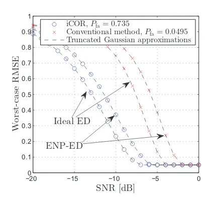
Fig. 1. Worst-case RMSE,M= 1000, ideal ED withN= 100, ENP-ED withN= 100andK= 100,λW,RMSE= 0.05, Bernoulli model.
L = 1. Signal following the IEEE 802.11b standard is generated with a signal generator with a random payload. The reference COR Ψ = 0.40 is obtained by controlling the idle time between packets. The signal generator output is connected to a channel emulator input and the channel emulator output is connected to the measurement system input. With this approach measurements can be controlled with a high precision. Both AWGN and time-variant and frequency selective ETSI BRAN WLAN model A (corresponding to a typical office environment) channels are utilized. We measured 100 000 noise-only ED decision variables in a measurement chamber shielded from radio signals (matched load was used to further suppress any possible signals) to estimateσ2nand to set threshold for any targetPfa with (15).
B. iCOR vs Conventional Method
Figs. 1 and 2 show the worst-case RMSE for iCOR and conventional COR estimation methods for M = 1000 obser-vations and the ED (both ideal and ENP-ED with K = 100) with N = 100 complex samples used for each observation. Results show an excellent agreement of the truncated Gaussian approximation to the exact theoretical results by (28). SinceM is large, the used occupancy model is not significantly affecting the results. The noise estimation in the ENP-ED results in a few dB loss.
[image:7.612.69.273.139.335.2]The gain of the proposed iCOR method for λW,RMSE = 0.05(Fig. 1) is around 4 dB at the worst-case RMSE = 0.1,
TABLE I. MEASUREMENT SETUP
Instrument Agilent N6841A
Center frequency 2450 MHz
Frequency span 100 MHz
Resolution bandwidth 242.27 kHz Frequency bin separation 109.375 kHz
Window type Gausstop window
NFFT (in a frequency segment) 256
L 1
Digital IF bandwidth 20 MHz Number of frequency points 916
Sweep time ≈10 ms
Filter Creowave filter
Band-pass frequency range 2400–2500 MHz Insertion loss (pass-band) 0.8 dB
Rejection bands 0–2300 MHz & 2600–5500 MHz Rejection at rejection bands ≥90 dB
Low noise amplifier Mini-Circuits ZRL-3500
Frequency range 700–3500 MHz
Gain (2.45 GHz) 19.5 dB
Noise Figure (2.45 GHz) 2.5 dB
Signal generator Agilent E4438C ESG
Signal type IEEE 802.11b
Actual COR levelΨ 0.40
Data rate 11 Mbit/sec
Total packet size 1508 bytes
Center frequency 2472 MHz
Channel emulator EB Propsim F8
Channel types AWGN
ETSI WLAN A Channel for COR estimation IEEE 802.15.4 channel
Number of frequency bins|Θs| 18
Bandwidth 2 MHz
Offset to the signal center freq. 7 MHz
and around 7 dB at RMSE = 0.8. For λW,RMSE = 0.02 in Fig. 2 the iCOR gain is around 2 dB at RMSE = 0.1, and around 4 dB at RMSE = 0.8. Therefore, the improvement observed is around 4–7 dB in Fig. 1 and 2–4 dB in Fig. 2.
[image:7.612.293.568.142.556.2]−20 −15 −10 −5 0 0
0.1 0.2 0.3 0.4 0.5 0.6 0.7 0.8 0.9 1
SNR [dB]
W
o
rs
t-ca
se
R
M
S
E
iCOR,Pfa= 0.209
Conventional method,Pfa= 0.019
Truncated Gaussian approximations
[image:8.612.348.540.53.218.2]ENP-ED Ideal ED
Fig. 2. Worst-case RMSE,M= 1000, ideal ED withN= 100, ENP-ED withN= 100andK= 100,λW,RMSE= 0.02, Bernoulli model.
0 0.2 0.4 0.6 0.8 1
0 0.1 0.2 0.3 0.4 0.5 0.6 0.7 0.8 0.9 1
Pfa
W
o
r
s
t
-c
a
s
e
R
M
S
E
iCOR
Conventional method
Pd−Pfa
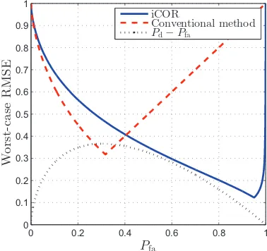
Fig. 3. Worst-case RMSE as a function ofPfa,SNR =−10dB,M= 1000,
ideal ED withN= 100, Bernoulli model.
λW,RMSE = 0.02, the conventional method can use Pfa = 0.019 while iCOR can use Pfa= 0.209 (approximation (51) gives 0.29). Fig. 3 shows the worst-case RMSE as a function of Pfa for SNR = −10 dB. We can see that the optimal Pfa for the conventional method is around the point where Pd −Pfa reaches its maximum. However, since the iCOR can suppress the effect of Pfa, its optimal point is at Pfa of more than 0.9. Since the worst-case RMSE with Pd = 1 is constrained, neither of these methods is able to use their optimalPfa(for this particularSNRlevel). However, the iCOR can use Pfa = 0.735, which is much closer to its optimal point than the conventional method tied to a very small value (Pfa= 0.0495).
In Fig. 4, we show the RMSE contour as the functions of SNR and Ψ. The worst-case RMSE can be obtained by selecting for each SNR the highest value in the vertical direction corresponding to selecting the value of Ψ leading
0.05
0.05
0.05
0.1
0.1
0.1
0.2
0.2
0.2
0.3
0.3
0.3
0.4
0.4 0.4
0.5
0.5
SNR [dB]
Ψ
a) Conventional method,Pfa= 0.0495
−20 −15 −10 −5 0
0 0.5 1
0
0.05
0.05 0.05
0.1
0.1 0.1
0.2
0.2
0.3
0.3
0.4
0.4
0.5
0.5
SNR [dB]
Ψ
b) iCOR,Pfa= 0.735
−20 −15 −10 −5 0
[image:8.612.81.269.54.232.2]0 0.5 1
Fig. 4. Contour plot of RMSE vsSNRandΨ,M = 1000, ideal ED with
N= 100, a) conventional method, b) iCOR,λW,RMSE= 0.05, Bernoulli
model.
−20 −15 −10 −5 0
0 0.1 0.2 0.3 0.4 0.5 0.6 0.7 0.8 0.9 1
SNR [dB]
W
or
st
-c
as
e
M
A
E
iCOR,Pfa= 0.817
Conventional method,Pfa= 0.05
Truncated Gaussian approximations
Fig. 5. Worst-case MAE,M= 1000, ideal ED withN= 100,λW,MAE= 0.05, Bernoulli model.
to the highest RMSE.
Fig. 5 shows the worst-case MAE for the iCOR and the conventional COR estimation methods for M = 1000 obser-vations and ideal ED with N = 100 complex samples used for each observation. The constraint value used isλW,MAE= 0.05. The gain of the proposed iCOR method is around 4–7 dB. By comparing Fig. 5 with the results for ideal ED in Fig. 1 we observe that the results for MAE and RMSE do not have significant differences.
C. Effect of the Signal Occupancy Model
[image:8.612.351.538.268.442.2] [image:8.612.80.269.275.453.2]−20 −15 −10 −5 0 0
0.1 0.2 0.3 0.4 0.5 0.6 0.7 0.8 0.9 1
SNR [dB]
W
o
rs
t-ca
se
R
M
S
E
iCOR
Conventional method
Truncated Gaussian approximations
m-out-of-M model
[image:9.612.351.540.52.233.2]Bernoulli model
Fig. 6. Worst-case RMSE,M= 110, ideal ED withN= 100,λW,RMSE= 0.05, Bernoulli andm-out-of-M models.
model, but it can be up to 4 dB, which is a remarkable improvement, under them-out-of-M model. Thus, for them -out-of-M model the iCOR significantly improves performance compared to the conventional method. The reason for this behaviour lies in the allowedPfa values. The allowedPfafor the conventional method is 0.0279 for the Bernoulli model and 0.0459 for the m-out-of-M model. For the iCOR solutions, the allowedPfais 0.047 for the Bernoulli model and 0.239 for them-out-of-M model. The truncated Gaussian approximation still gives very good accuracy.
D. Experimental Results
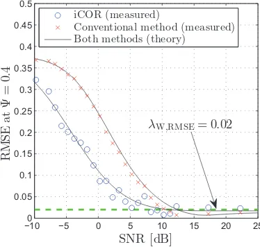
The measurement results in Fig. 7 for the AWGN channel validate the iCOR method and also show an excellent fit between the experimental and theoretical results. Small dif-ferences result from the random signal model not being exact and from the limited number of measurement samples.
In Fig. 7, for SNR values around 5 dB, it is observed that the theoretical RMSE for the conventional method increases with the SNR and then converges to a final level. Usually, the RMSE is a non-increasing function of the SNR. This behavior is caused by the false alarms. WhenPd= 1, the false alarms can only be harmful. WhenPdis close to one, the false alarms can offset the loss due missing actual signals.
The RMSE at high SNR can be smaller for the conventional method. The reason is the fact that we limit the worst-case RMSE to the worst actual COR level. The conventional method has its worst RMSE, when the actual COR is around zero, but the iCOR estimate has its worst RMSE at a higher COR level. The value Ψ = 0.4utilized in the experiments is closer to the COR level leading to the worst-case RMSE for the iCOR than that for the conventional method.
Fig. 8 shows the results with the ETSI BRAN A WLAN channel model. For the theoretical results we use the Rayleigh fading channel model providing excellent fit to the measure-ments.
−15 −10 −5 0 5
0 0.05 0.1 0.15 0.2 0.25 0.3 0.35 0.4 0.45 0.5
SNR [dB]
R
M
S
E
at
Ψ
=
0
.
4
iCOR (measured)
Conventional method (measured) Both methods (theory)
[image:9.612.81.269.54.232.2]λW,RMSE= 0.02
Fig. 7. Real measurement and theoretical results, AWGN channel (theory and measurement), 802.11b signal (measurement), Gaussian signal (theory),
Ψ = 0.4,λW,RMSE= 0.02(shown with a green dashed line),M= 5000.
−10 −5 0 5 10 15 20 25
0 0.05 0.1 0.15 0.2 0.25 0.3 0.35 0.4 0.45 0.5
SNR [dB]
R
M
S
E
at
Ψ
=
0
.
4
iCOR (measured)
Conventional method (measured) Both methods (theory)
λW,RMSE= 0.02
Fig. 8. Real measurement and theoretical results, ETSI BRAN-A WLAN channel (measurement), Rayleigh fading (theory), 802.11b signal (measure-ment), Gaussian signal (theory),Ψ = 0.4,λW,RMSE= 0.02(shown with a
green dashed line),M= 5000.
VIII. OPTIMIZEDMAPPINGFUNCTIONS
We may ask: is the mapping function (48) for the proposed iCOR method optimal? We already know that it is the MLE for Pd = 1. However, this does not imply the optimality for the RMSE. In this section, we compare the iCOR to two differently optimized mapping functions with them-out-of-M model.
A. RMSE-optimal forPd= 1
[image:9.612.350.537.288.466.2]0 20 40 60 80 100 0
0.1 0.2 0.3 0.4 0.5 0.6 0.7 0.8 0.9 1
k
ˆΨ
90 95 100
0.9 0.95 1
k
ˆΨ
RMSE-optimal forPd= 1,Pfa= 0.276 iCOR,Pfa= 0.222
Conventional method,∀Pfa
Optimal linear,Pfa= 0.2029
[image:10.612.84.268.52.208.2]zo om
Fig. 9. Mapping function fromktoΨˆfor RMSE-optimal weights forPd= 1,
iCOR, conventional method, and optimized linear weights,M = 100, ideal ED withN= 100,m-out-of-M model,λW,RMSE= 0.05.
for a given Pfa is
min
Ξ
max
m∈{0,1,···,M}
∑
k∈{0,1,···,M} pk
(
ξk− m M
)2
, (53)
whereΞ = [ξ0ξ1 · · · ξM] corresponds to an arbitrary vector mapping k to Ψˆ and pk is found with (23) assuming Pd = 1. We solve the optimization problem and increase the target Pfa value as long as the worst-case RMSE-optimal mapping function satisfies the λW,RMSE constraint. This leads to the mapping function allowing the highest possible Pfa for the specified constraint λW,RMSE.
B. Optimized Linear
We numerically optimize the coefficients a1 and a0 of the linear function (30). The optimization target was to find the coefficients that minimize the required SNRfor reaching the worst-case RMSE of0.1 (corresponding to2λW,RMSE) while satisfying the constraintλW,RMSE. The aim here is to not only optimize for Pd = 1but also to consider weaker signals for whichPd<1.
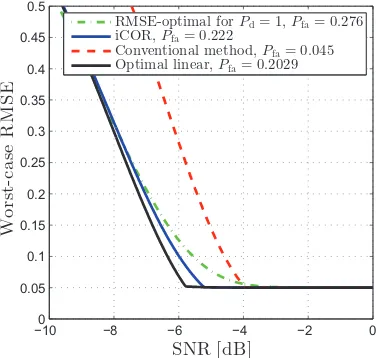
C. Results for Mapping Function and Worst-case RMSE ForM = 100andλW,RMSE= 0.05, the resulting mapping functions are presented in Fig. 9. The RMSE-optimal weights for Pd= 1are slightly non-linear and allow using the highest Pfa from all the considered methods as it should be, because this was the optimization target. However, as shown in Fig. 10, even with the higher Pfa, the performance of the RMSE-optimal mapping function for Pd = 1 is worse for medium signal power levels than the performance of the iCOR method. This is because the mapping function optimized for Pd= 1is not necessarily optimal for lower SNR values. The RMSE-optimal mapping function for Pd = 1 uses Ψˆ less than 1 even whenk=M. When the signal power is reduced, signals are not always detected, i.e., Pd < 1. In this case, it would be better to use higher output COR values to compensate for
−10 −8 −6 −4 −2 0
0 0.05 0.1 0.15 0.2 0.25 0.3 0.35 0.4 0.45 0.5
SNR [dB]
W
o
rs
t-ca
se
R
M
S
E
RMSE-optimal forPd= 1,Pfa= 0.276 iCOR,Pfa= 0.222
Conventional method,Pfa= 0.045 Optimal linear,Pfa= 0.2029
Fig. 10. Worst-case RMSE for RMSE-optimal weights forPd= 1, iCOR,
conventional method, and optimized linear weights, ideal ED withN= 100,
m-out-of-M model,λW,RMSE= 0.05.
the undetected signals. In fact, the optimized linear mapping function is doing exactly this. It has the highest output COR from all the considered methods for large values of k. The iCOR was also found assumingPd= 1(it is MLE forPd= 1). However, its output is significantly larger at high values ofk than the RMSE-optimal mapping function forPd= 1, leading to better performance whenPd<1. The conventional method also has large output values at high values ofk, but it greatly suffers from too large output when k is small (leading to no suppression of false alarms). The linear mapping function has a slightly better performance than iCOR. However, the performance of the iCOR is close and a significant amount of computation is required to find the optimal linear mapping function. Thus, the iCOR presents an excellent compromise between the complexity and performance.
IX. CONCLUSION
[image:10.612.351.539.53.232.2]APPENDIXA
Proof that the maximum allowed Pfa for conventional COR estimation under Bernoulli model is(42): The RMSE is given in (39). For Pd= 1 and given Pfa, the extremum point obtained by solving d[mse(Ψ)]dΨ = 0 (extremum points are the same for mseandrmse) is
Ψ (Pfa) = 3Pfa+ 2M P 2 fa−2P
2 fa−1 4Pfa+ 2M P2
fa−2Pfa2−2
(54)
which is valid, i.e., Ψ∈[0 1], if
0≤Pfa≤
√
8M + 1−3
4 (M −1) (55)
The MSE for the extremum point is
− (Pfa−1)
2
4M(2Pfa+M P2 fa−P
2 fa−1)
(56)
The MSE for the boundary point Ψ = 0is
Pfa
M +P
2 fa
(
1− 1 M
)
(57)
As the extremum point MSE is always greater than or equal to MSE of Ψ = 0 (within its validity region), we get that the worst-case MSE is
− (Pfa−1)2 4M(2Pfa+M Pfa2−P
2 fa−1)
0≤Pfa≤
√
8M+1−3 4(M−1) Pfa
M +P 2 fa−
P2 fa
M otherwise
(58)
This results into maximum allowed Pfagiven by (42).
REFERENCES
[1] “Expanding America’s leadership in wireless innovation,” The White House, Washington D.C., Jun. 2013.
[2] Q. Zhao and B. M. Sadler, “A survey of dynamic spectrum access,” IEEE Signal Process. Mag., vol. 24, no. 3, pp. 79–89, May 2007. [3] Federal Communications Commission, “Second memorandum opinion
and order, FCC 10-174,” Sep. 2010.
[4] I. F. Akyildiz, W.-Y. Lee, M. C. Vuran, and S. Mohanty, “A survey on spectrum management in cognitive radio networks,”IEEE Commun. Mag., vol. 46, no. 4, pp. 40–48, Apr. 2008.
[5] T. Y¨ucek and H. Arslan, “A survey of spectrum sensing algorithms for cognitive radio applications,” IEEE Commun. Surveys Tuts., vol. 11, no. 1, pp. 116–130, 2009.
[6] M. L´opez-Ben´ıtez and F. Casadevall, “Signal uncertainty in spectrum sensing for cognitive radio,”IEEE Trans. Commun., vol. 61, no. 4, pp. 1231–1241, Apr. 2013.
[7] A. Mariani, A. Giorgetti, and M. Chiani, “Effects of noise power estimation on energy detection for cognitive radio applications,”IEEE Trans. Commun., vol. 59, no. 12, pp. 3410–3420, Dec. 2011. [8] Y. Zeng, Y.-C. Liang, A. T. Hoang, and R. Zhang, “A review on
spec-trum sensing for cognitive radio: Challenges and solutions,”EURASIP J. Adv. Signal Process, vol. 2010, Jan. 2010.
[9] M. Wellens, A. Baynast, and P. M¨ah¨onen, “On the performance of dynamic spectrum access based on spectrum occupancy statistics,”IET Commun., vol. 2, no. 6, pp. 772–782, Jul. 2008.
[10] K. Umebayashi, Y. Suzuki, and J. Lehtom¨aki, “Dynamic selection of CWmin in cognitive radio networks for protecting IEEE 802.11 primary users,” inProc. CROWNCOM, Jun. 2011, pp. 266–270.
[11] “1000x: More spectrum-especially for small cells,” Tech. Rep., Nov. 2013. [Online]. Available: http://www.qualcomm.com/media/ documents/files/1000x-more-spectrum-especially-for-small-cells.pdf [12] K. Chintalapudi, B. Radunovic, V. Balan, M. Buettener, S. Yerramalli,
V. Navda, and R. Ramjee, “WiFi-NC: WiFi over narrow channels,” in Proc. NSDI, 2012.
[13] M. L´opez-Ben´ıtez and F. Casadevall, “Methodological aspects of spec-trum occupancy evaluation in the context of cognitive radio,”European Trans. Telecommun., vol. 21, no. 8, pp. 680–693, Dec. 2010. [14] A. D. Spaulding and G. H. Hagn, “On the definition and estimation
of spectrum occupancy,”IEEE Trans. Electromagn. Compat., vol. 19, no. 3, pp. 269–280, Aug. 1977.
[15] R. Bacchus, T. Taher, K. Zdunek, and D. Roberson, “Spectrum utiliza-tion study in support of dynamic spectrum access for public safety,” in Proc. DySPAN, Apr. 2010.
[16] J. Lehtom¨aki, R. Vuohtoniemi, and K. Umebayashi, “On the measure-ment of duty cycle and channel occupancy rate,”IEEE J. Sel. Areas Commun., vol. 31, no. 11, pp. 2555–2565, Nov. 2013.
[17] M. Biggs, A. Henley, and T. Clarkson, “Occupancy analysis of the 2.4 GHz ISM band,”IEE Proc. Commun., vol. 151, no. 5, pp. 481–488, Oct. 2004.
[18] M. Wellens and P. M¨ah¨onen, “Lessons learned from an extensive spectrum occupancy measurement campaign and a stochastic duty cycle model,”Mobile Netw. Appl., vol. 15, no. 3, pp. 461–474, 2010. [19] M. Wellens, J. Riihij¨arvi, and P. M¨ah¨onen, “Empirical time and
fre-quency domain models of spectrum use,” Phys. Commun., vol. 2, no. 1-2, pp. 10–32, Mar. 2009.
[20] M. L´opez-Ben´ıtez and F. Casadevall, “Time-dimension models of spectrum usage for the analysis, design, and simulation of cognitive radio networks,”IEEE Trans. Veh. Technol., vol. 62, no. 5, pp. 2091– 2104, Jun. 2013.
[21] S. Wang, F. Patenaude, and R. J. Inkol, “Computation of the normalized detection threshold for the FFT filter bank-based summation CFAR detector,”Journal of Computers, vol. 2, no. 6, pp. 35–48, Aug. 2007. [22] J. Naganawa, H. Kim, S. Saruwatari, H. Onaga, and H. Morikawa,
“Distributed spectrum sensing utilizing heterogeneous wireless devices and measurement equipment,” inProc. DySPAN, May 2011, pp. 173– 184.
[23] J. J. Lehtom¨aki, R. Vuohtoniemi, K. Umebayashi, and J.-P. M¨akel¨a, “Energy detection based estimation of channel occupancy rate with adaptive noise estimation,”IEICE Trans. Commun., vol. E95-B, no. 4, pp. 1076–1084, Apr. 2012.
[24] K. Umebayashi, R. Takagi, N. Ioroi, J. Lehtom¨aki, and Y. Suzuki, “Duty cycle and noise floor estimation with Welch FFT for spectrum usage measurements,” inProc. CROWNCOM, Oulu, Finland, Jun. 2014. [25] M. Abramowitz and I. Stegun,Handbook of Mathematical Functions.
New York: Dover, 1964.
[26] J. J. Lehtom¨aki, M. Juntti, and H. Saarnisaari, “CFAR strategies for channelized radiometer,”IEEE Signal Process. Lett., vol. 12, no. 1, pp. 13–16, Jan. 2005.
[27] F. J. Harris, “On the use of windows for harmonic analysis with the discrete Fourier transform,”Proc. IEEE, vol. 66, no. 1, pp. 51–83, 1978. [28] J. P. Imhof, “Computing the distribution of quadratic forms in normal
variables,”Biometrika, vol. 48, no. 3/4, pp. 419–426, Dec. 1961. [29] N. Johnson, S. Kotz, and N. Balakrishnan, Continuous univariate
distributions. Wiley, 1994, vol. 1.