This is a repository copy of
Robust control of uncertain multi-inventory systems via Linear
Matrix Inequality
.
White Rose Research Online URL for this paper:
http://eprints.whiterose.ac.uk/89749/
Version: Accepted Version
Proceedings Paper:
Bauso, D., Giarré, L. and Pesenti, R. (2008) Robust control of uncertain multi-inventory
systems via Linear Matrix Inequality. In: Proceedings of the American Control Conference.
2008 American Control Conference, June 11-13, 2008, Westin Seattle Hotel, Seattle,
Washington, USA. Institute of Electrical and Electronics Engineers , 4081 - 4086. ISBN
9781424420797
https://doi.org/10.1109/ACC.2008.4587132
[email protected] https://eprints.whiterose.ac.uk/ Reuse
Unless indicated otherwise, fulltext items are protected by copyright with all rights reserved. The copyright exception in section 29 of the Copyright, Designs and Patents Act 1988 allows the making of a single copy solely for the purpose of non-commercial research or private study within the limits of fair dealing. The publisher or other rights-holder may allow further reproduction and re-use of this version - refer to the White Rose Research Online record for this item. Where records identify the publisher as the copyright holder, users can verify any specific terms of use on the publisher’s website.
Takedown
If you consider content in White Rose Research Online to be in breach of UK law, please notify us by
Robust control of uncertain multi-inventory systems via Linear Matrix
Inequality
D. Bauso, L. Giarr´e and R. Pesenti
Abstract— We consider a continuous time linear multi– inventory system with unknown demands bounded within ellipsoids and controls bounded within ellipsoids. We address the problem ofǫ-stabilizing the inventory since this implies some reduction of the inventory costs. As main result, we provide conditions under which ǫ-stabilizability is possible through a saturated linear state feedback control. All the results are based on a Linear Matrix Inequalities (LMIs) approach.
I. INTRODUCTION
We consider a continuous time linear multi–inventory sys-tem with unknown demands bounded within ellipsoids and controls bounded within ellipsoids. The system is modelled as a first order one integrating the discrepancy between controls and demands at different sites (buffers). Thus, the state represents the buffer levels. We wish to study conditions under which the state can be driven within an a-priori chosen target set through a saturated linear state feedback control. Let ǫ be a maximal dimension of the target set, the above problem corresponds toǫ-stabilizing the state.
Motivations for ǫ-stabilizing the state derive from the benefits associated to keeping the state and consequently also the inventory costs bounded. This work is in line with some recent literature on robust optimization [1], [6] and control [2] of inventory systems. Here as well as in [2] we focus on saturated linear state feedback controls since such controls arise naturally in any system with bounded controls. The main results of this work can be summarized as follows. Initially we introduce the necessary and sufficient conditions for theǫ-stabilizability in the form of an inclusion between convex sets. In the case where both demands and controls are bounded within polytopes, it is well known that verifying such conditions is NP-hard [9]. Here, we prove that verification becomes easy when both demands and controls are bounded within ellipsoids. This is possible by rewriting the inclusion between ellipsoids in terms of unconstrained quadratic maximization.
We first characterize invariant sets through a fourth degree condition. As verifying such a condition is difficult, we then propose the best quadratic approximation of the same condition. We proceed by describing the region of linearity
This work was supported in part by PRIN “Advanced control and identification techniques for innovative applications”, and PRIN “Analysis, optimization, and coordination of logistic and production systems”.
D. Bauso is with Dipartimento di Ingegneria Informatica-DINFO, Uni-versit`a di Palermo, 90128 Palermo, Italy, (e-mail: [email protected])
L. Giarr´e is with Dipartimento di Ingegneria dell’Automazione e dei Sistemi-DIAS, Universit`a di Palermo, 90128 Palermo, Italy (e-mail: [email protected])
R. Pesenti is with Dipartimento di Matematica Applicata-DMA, Univer-sit`a di Venezia, 30123 Venezia, Italy, (e-mail: [email protected])
of the control and conclude by providing LMI conditions on the target set under which the saturated controlǫ-stabilizes the system. The case where demands are bounded within ellipsoids and controls are bounded within polytopes is an open problem and sufficient LMI conditions to solve it are presented in [3].
All the results are based on a Linear Matrix Inequalities (LMIs) approach in line with the recent work [7] on inven-tory/manufacturing systems.
This paper is arranged as follows. In Section II, we formu-late the problem. In Section III, we introduce necessary and sufficient conditions for the admissibility of the problem. In Section IV we study the problem with ellipsoidal constraints. In Section V, we provide numerical illustrations. Finally, in Section VI, we draw some conclusions.
II. PROBLEMFORMULATION
Consider the continuous time linear multi–inventory sys-tem
˙
x(t) =Bu(t)−w(t), (1) where x(t) ∈ IRn is a vector whose components are the buffer levels,u(t)∈IRm is the controlled flow vector,B∈
Qn×m, with m ≥ n and rank(B) = n is the controlled
process matrix andw(t)∈IRn is the unknown demand. To
model backlog x(t) may be less than zero. Demands and controls are bounded within ellipsoids, i.e.,
w(t) ∈ W={w∈Rn:wTRww≤1} (2)
u(t) ∈ U ={u∈Rm:uTR
uu≤1}. (3)
For any positive definite matrix P ∈ Rn×n, define the
function V(x) = xTP x and the ellipsoidal target set Π =
{x ∈ IRn : V(x) ≤ 1}. In addition, for any matrix K ∈
Rn×n, define as saturated linear state feedback control any
policy
u=sat{−Kx}= ½
−Kx ifKx∈ U
u(x)∈∂U otherwise (4) where hereafter∂F indicates the frontier of a given setF.
Problem 1: (ǫ-stabilizing) Given system (1), find condi-tions on the positive definite matrix P ∈ Rn×n, under
which there exists a saturated linear state feedback control
u = sat{−Kx} such that it is possible to drive the state
x(t)within the target setΠ.
Solving the above problem corresponds toǫ-stabilizing the statexwhere the relation betweenǫ andΠ is
ǫ:= max
u
1u
2 [image:3.612.109.249.54.119.2]w
Fig. 1. Graph with one node and two arcs.
Example 1: Throughout this paper we consider, as illus-trative example, the graph with one node and two arcs depicted in Fig. 1. The incidence matrix is B = [1 1]. The continuous time dynamics is
˙
x(t) = [1 1] | {z }
B
·
u1(t)
u2(t) ¸
| {z }
u
−w=u1(t) +u2(t)−w(t),
with demand bounded in the ellipsoid
w2≤1
and with the following either ellipsoidal constraints on the control u
(u1+u2)2≤1, (6) Finally, the target set is the sphere of unitary radius Π =
{x∈R:x2≤1}.
III. STABILITY NECESSARY AND SUFFICIENT CONDITIONS
System (1) isǫ-stabilizable if and only if for all w∈ W, there existsu∈int{U}such that Bu=w (see, e.g., [4]). For the short of notation, the previous condition is usually expressed as
BU ⊃ W. (7)
Deciding whether (7) holds is NP-hard, whenU andW are polytopes. Here, we prove that verifying (7) becomes easy when both U and W are ellipsoids. Observe that we can rewrite Bu =w as uB =B−1w− B−1N u
N, where B =
[B|N]beingBa basis ofB andN the remaining columns of
B, correspondinglyuBare thencomponents ofuassociated to the basis B and uN are the m−n components of u
associated to the columns inN.
As we observe that (7) is equivalent to
max
w∈W u∈Rminm
:Bu=wuRuu <1,
Condition (7) holds if and only if
max
w∈WuNmin∈Rm−nf(uB(w, uN), uN) =
=£wTB−T−uT
NNTB−T|uTN
¤
Ru (8)
·
B−1w− B−1N u
N
uN
¸
<1
When we consider the illustrative example in Section 1, we have B= [1],N= [1]then problem (9) becomes
max
−1≤w≤1umin2∈R
f(uB(w, u2), u2) = = [w−u2|u2]
· 1 0 0 1
¸ ·
w−u2
u2 ¸
= (w−u2)2+u22<1
Now consider, function f(uB(w, uN), uN). It is a
dif-ferentiable convex function in uN. Then, for any w ∈ W
we can analytically determine the best response u∗
N(d) =
argminuN∈Rm−nf(u
B(w, uN), uN), by imposing
∇uNf(uB(w, uN), uN) =
2£−NTB−T|I¤R u
·
B−1w− B−1N u
N
uN
¸ = 0,
whereIis the(m−n)×(m−n)identical matrix. We obtain
u∗
N(w) =−M w,
where0is the (m−n)×nnull matrix and
M = µ
£
−NTB−T
|I¤Ru
·
−B−1N
I
¸¶−1
£
−NTB−T|I ¤R u
·
B−1 0
¸
.
In the example under consideration, we have
u∗
2(w) = − µ
[−1|1] ·
1 0 0 1
¸ ·
−1 1
¸¶−1 [−1|1] ·
1 0 0 1
¸ · 1 0
¸
w= w
2.
For anyw∈ W the minimal value off(uB(w, uN), uN)is
f(uB(w, u∗N(w)), u∗N(w)) =w∗TΦw∗,
where
Φ = [B−T +MTNTB−T| −MT]
| {z }
HT
Ru
·
B−1+B−1N M
−M
¸
| {z }
H
=HTR
uH (9)
is a positive definite n×n matrix, as M is full rank. So far, we have shown that we can find the optimal value of problem (9) by solving problem
max
w∈Ww
TΦw,
(10)
and checking that the optimal value is less than one. We are ready to observe that problem (10) is easy as it reduces to determining the eigenvectors of ann×nmatrix.
Theorem 3.1: System (1) is ǫ-stabilizable if and only if w∗TΦw∗ < 1, for all w∗ eigenvectors associated to
the maximum eigenvalue of matrix R−1
w Φ whose weighted
quadratic normw∗TR
ww∗ is equal to 1.
Proof: AswTΦw is convex, its optimal valuew∗ lays
on the frontier ∂W of the set W, i.e., for w∗TR ww∗ =
1. Imposing the Karush Kuhn Tucker first order optimality condition, we obtain2(Φ−λRw)w∗= 0. Then the optimal
values of w∗ are some of the matrix R−1
w Φ eigenvectors
whose weighted quadratic normw∗TR
ww∗ is equal to 1. In
particular,w∗are the eigenvectors associated to the maximal
eigenvalues ofR−1
w Φ.
In the example under considerationΦ =£1 2 ¤
andw∗=±1
then w∗TΦw∗ = 1
In the following we discuss for which initial state the system is certainlyǫ-stabilizable through a (pure) linear state feedback control; hence we show that if we saturated the previous linear policy the system is ǫ-stabilizable for any initial state.
IV. ELLIPSOIDAL CONSTRAINTS
Let us start by considering only the constraints (2) onw
and neglect the ellipsoidal constraints (3) on u. Among the saturated linear state feedback control (4) we prove that we can solve Problem 1 using controls of typeu=sat{−kHx}, withk∈RandH ∈Rn as defined in (9). Note that matrix
H is a right inverse ofB, that isBH=I. We motivate the choice ofu=sat{−kHx}withH as defined in (9) as such a control describes the best response ofuunder the worstw
as proved in the previous section. Also, note that the scalar
k∈Rmust be lower than a certain value, which means that we cannot use a bang-bang control. This is motivated by the following reason. If we use a controlu=sat{−kHx}, then the necessary and sufficient condition (7) becomes
BUlin ⊃ W (11)
where
Ulin={u∈Rm: u=−kHx, k2xTHTRuHx≤1}.
Following the derivation of (10) in the previous Section, we have that (11) holds if and only if
k2w∗TΦw∗<1.
For k = 1 the above condition holds true as it reduces to (10). Obviously, the valuekˆ=qw∗T1Φ
w∗ is an upper bound fork, namely, we must chooseksuch thatk <ˆkif we wish the necessary and sufficient condition (11) be satisfied.
With the above considerations in mind, we can conclude that the dimensions of the target Π where it is possible to drive the state are lower bounded.
Denote byλmax(Z) the maximum eigenvalue of a given
matrixZ. In the following theorem we prove thatV˙(x)<0 within a given set (invariant set). This result will allow exploiting V(x) as a Lyapunov function to prove the con-vergence to the target setΠ.
Theorem 4.1: Consider system (1) subject to the only ellipsoidal constraints (2) on w, and controlled via linear state feedback u = −kHx, with H such that BH = I. Then condition V <˙ 0holds if and only if
k2(xTP x)2−xTP R−1
w P x >0. (12)
Proof: For H such that BH =I, condition V <˙ 0 is equivalent to
2kxTP x+ 2wTP x >0. (13) We aim at proving thatV <˙ 0holds for anyxexternal to an appropriate smooth closed surface. To do this, we look for anx∈Rn inducing a solution strictly greater than zero for
the following problem
min
w∈Wζ(x, w) = 2kx
TP x+ 2wTP x. (14)
Asζ(x, w) is linear in w, the optimalw∗ must lay on the
boundary of set W. The Karush Kuhn Tucker conditions impose thatP x=−λRww∗ for someλ≥0, that is w∗=
−λ1R−
1
w P x. Note that beingP full rank, it necessarily holts
thatλ 6= 0 for all x 6= 0. Then, ζ(x, w∗) = 2kxTP x−
2
λxTP R−
1
w P x > 0. As w∗ lays on the boundary of W,
we have w∗TR
ww∗ = x T
P R−1
w P x
λ2 = 1 from which λ =
p
xTP R−1
w P x. Hence,ζ(x, w∗)>0, and therefore also (13)
holds, if and only if (12) holds.
We now exploit V(x) = xTP x as a Lyapunov function
to prove the convergence to the target setΠ. We determine under which conditions onP andkwe have thatV <˙ 0or, equivalently, inequality (12) hold for anyx6∈Π.
When P = νRw, (12) becomes k2xTP x > ν. Then, in
this case, we can useV(x)to prove the convergence of the system toΠ for k2≥ν.
In the following, we consider the general case whenP6=
νRw.
Lemma 4.2: Consider system (1) subject to the only el-lipsoidal constraints (2) onw, and controlled via linear state feedback u = −kHx, with H such that BH = I. Then,
k2(xTP x)2−xTP R−1
w P x >0 holds for anyx6∈Π if and
only ifk2−xTP R−1
w P x≥0 holds for anyx∈∂Π.
Proof: (Necessity). Assume that there exists xˆ ∈ ∂Π such that k2 −xTP R−1
w P x < 0. Then, there also exists
a ball Ball(ˆx, r) centered in xˆ with a sufficiently small radius r > 0 such that for all x ∈ Ball(ˆx, r) we have
k2−xTP R−1
w P x <0. This implies that there existx6∈Π
for which condition (12) does not hold. (Sufficiency). Assume that k2−xTP R−1
w P x ≥ 0 holds
for any x ∈ ∂Π. By contradiction, consider xˆ 6∈ Π, i.e., ˆ
xTPxˆ =ρ > 1, such that k2(ˆxTPxˆ)2−xˆTP R−1
w Px <ˆ 0,
that is k2ρ2 −xˆTP R−1
w Px <ˆ 0. Then, there exists x˜ =
ˆ
x
√ρ ∈∂Πsuch thatk2ρ2−ρx˜TP R−1
w Px <˜ 0, that isk2ρ−
˜
xTP R−1
w Px <˜ 0. This latter result is contradictory as we
cannot havek2ρ <x˜TP R−1
w Px˜≤k2, forρ >1.
Lemma 4.3: Consider system (1) subject to the only el-lipsoidal constraints (2) onw, and controlled via linear state feedback u=−kHx, with H such that BH =I. We can use V(x) to prove the convergence of the system toΠ for
k2≥λmax(R−w1P).
Proof: Conditionk2−xTP R−1
w P x≥0 holds for any
x∈ ∂Π if and only if minx∈∂Π{k2−xTP R−w1P x} ≥ 0.
Imposing the Karush Kuhn Tucker first order optimality con-dition, we obtain2(P R−1
w P−λP)x∗= 0. Then the optimal
values of x∗ are some of the matrix R−1
w P eigenvectors
whose weighted quadratic norm x∗TP x∗ is equal to 1. In
particular, x∗ are the eigenvectors associated to the
maxi-mal eigenvalues of R−1
w P. For vectors x∗, condition k2−
x∗TP R−1
w P x∗ ≥0 becomes k2−λmax(R−w1P)x∗TP x∗≥
0, that isk2−λ
Observe that the system converges to the target setΠR=
{x : k2xTR
wx ≤ 1} as any feasible target set Π = {x :
xTP x≤1}, with k2≥λ
max(R−w1P)includesΠR. Indeed,
Π⊇ΠR if xTP x−k2xTRwx=xT(P−k2Rw)x≤0 or
equivalently if P−k2R
w¹0. In turn, the latter condition
is equivalent to R−1
w P −k2I ¹ 0 that certainly holds as
k2≥λ
max(R−w1P)
In the next theorem we introduce the constraints on controls (3). To this end, we need to define the family of ellipsoids
Σ0(ξ) ={x∈Rn:xTP x≤x(0)TP x(0) :=ξ} (15) parametrized inξ≥1.
Theorem 4.4: Given system (1), we can drive the state
x(t) from any initial value x(0) ∈ Σ0(ξ) to the target set Π via linear state feedback u = −kHx if the following conditions hold
k2≥λmax(Rw−1P) (16)
k2ξλmax(P−1Φ)≤1. (17)
Proof: By Lemma 4.3, under condition (16) it holds ˙
V(t)<0for all x(t)6∈Π and thenV(x)can be considered as a Lyapunov function for the convergence of the state to the set Π when the linear controlu= −kHx is implemented. ConditionV˙(t)<0also implies thatΣ0(ξ)is invariant with respect to the same linear feedback as ξ ≥1 which means Σ0(ξ)⊇Π. Then
max
t≥0 u
T(t)R
uu(t)≤ max x∈Σ0(ξ)
k2xTHTRuHx=
= max
x∈Σ0(ξ)
k2xTΦx=k2ξλ
max(P−1Φ).
Therefore the constraintu=−kHx(t)∈ U for all t≥0 is enforced if (17) holds true.
The following theorem provides a solution to Problem 1. Let us denote byX the set of statesxwhere we can define a linear controlu(x) =−kHx, i.e.,X ={x:−kHx∈ U}. Consider the saturated linear state feedback control of type
u(x) = (
−kHx if x∈X
−√ Hx
xT HT
RuHx if x6∈X .
(18)
Theorem 4.5: Given system (1), for any positive definite matrix P ∈ Rn×n satisfying condition (16), the saturated linear state feedback control (18) drives the statex(t)within the target setΠ for any initial statex(0).
Proof: By construction, u(x) is a continuous function withU as codmain. When we use such a control, we know that V˙(x) < 0 also holds for any x 6∈ Π, if Π ⊂ X and
k2≥λ
max(R−1P)(see Lemma 4.3).
First observe that, for all x ∈ ∂X, we have xTP x >
k2xTHTR
uHx = 1, where the latter inequality holds as
Π⊂X. Then, for anyx6∈X, that is fork2xTHTR uHx >
1, we have xTP x xT
HT
RuHx > k
2 ≥ λ
max(R−1P) since
bothxTP xandxTHTR
uHxare positive definite quadratic
forms.
α(10−2) 1 2 3 4 5 6 7 8 9
ξ 31 15 10 7.7 6.2 5.1 4.4 3.8 3.4
α(10−2) 10 15 20 25 30 35 40 45 50
ξ 3 2 1.5 1.2 1 0.8 0.7 0.6 0.6
TABLE I
DEPENDENCE OFξONαIN THE CASE WHERERu:=αIANDk= 1:
THE HIGHERαTHE BIGGER THE REGIONΣ0(ξ)AS IN(15)AND ALSO THE REGION OF LINEARITYX={x:−kHx∈ U}.
In Lemma 4.3, we have proved that V˙(x) < 0 for x ∈ X\Π. Now, we considerx6∈X. We haveV˙(x)<0if and only if−xTP Bu(x) +xTP w >0, for allw∈ W, that is
min
w∈W
(
xTP x
p
xTHTR uHx
+xTP w
)
>0 (19)
must hold. Applying the Karush-Kuhn-Tuker conditions, we transform (19) in x
T P x
√
xT HT
RuHx −
p
xTPTR−1
w P x > 0. In turn, the latter inequality
holds if xTxTP x HT
RuHx − λmax(R−
1P) > 0, as
xTPTR−1
w P x ≤ λmax(R−1P)xTP x. We then conclude
thatV˙(x)<0since x
T P x xT
HT
RuHx > k
2≥λ
max(R−1P).
Observe that the saturated linear state feedback control (18) is not decentralized in the sense that the genericith con-trolui in general depends on the demand at different nodes
and on the other controlsuj, j6=i. This is due to either the
structure of matrixH or the ellipsoidal constraints (3).
Example 2: Consider the graph depicted in Fig. 1, with one node and two arcs and incidence matrix B = [1 1]. Controls are subject to ellipsoidal constraints (6). Then we have, Rw = 1, Ru = I and Φ = 12. We can stabilize the system within Π = {x∈ R: x2 ≤1} for any initial state
x(0)≤√2 via a pure linear state feedback u=−kHx. To see this takeQ=I, and observe that the matrix inequality on
Q(??) is satisfied for anyk≥1. Furthermore, if we assume
k= 1, then from (17) we must have k2= 1≤ 2
ξ2 =
2
x(0)2.
V. NUMERICALILLUSTRATIONS
Consider the constrained dynamics (1)-(3) for the flow network system withn= 5nodes andm= 9arcs depicted in Fig. 2 and take without loss of generality Rw =I and
Ru=αI for different values ofα= 0.01, . . . ,0.5. Trivially,
the higher the value of the parameter α, the weaker the constraints on the control (3). Also, from condition (17), we have that the weaker the constraints (3), the bigger the region Σ0(ξ) as defined in (15) and also the region of linearity X = {x : −kHx ∈ U}. In Table I, we display the dependence ofξon increasing values ofαwhenk= 1.
2
3
4
5 1
8
1
2 5
6
4
7
[image:6.612.91.263.66.202.2]9 3
Fig. 2. Example of a system with5nodes and9arcs.
withk= 13,12,1 and matrixH ∈Rn defined as
H =
0 1 0 0 0
0 0 0.5 0 0
−0.1 0 0.5 0 0
−0.2 0 0 0 0
0 0 0 0 0
0 0 0.5 0 0 0.1 0 0 1 0 0.6 1 1 0 0 0.4 0 0 1 1
. (20)
Note that matrixH is a right inverse ofB, that isBH =I. Basically, the columns of the above matrix establish that i) the demand at node 2 is satisfied by a flow through arc 8 and 1, ii) the demand at node 3 is satisfied by a flow through arc 8, which splits in two equal parts, the first one going through arc 2 and the second one through arc 3 and 6, iii) the demand at node 4 is entirely satisfied by a flow through arc 9 and 7, iv) finally the demand at node 5 is satisfied by a flow through arc 9. Obviously, the first column has no particular meaning since the demand at node 1 is null.
[image:6.612.316.553.199.391.2] [image:6.612.79.256.277.394.2] [image:6.612.317.557.456.650.2]Now, we simulate the system with initial state x(0) = [0 4 4 4 4]T and random demand w(t) for (a) k = 1
3, (b)
k = 12 and (c) k= 1. Demand w(t) is randomly extracted from the set{w(1), w(2), w(3), w(4)} with uniform probabil-ity where
w(1)= [0 ±1 0 0 0]T w(2) = [0 0 ±1 0 0]T
w(3)= [0 0 0 ±1 0]T w(4)= [0 0 0 0 ±1]T.
Actually, imposing a maximal (in this case the maximal demand componentwise is1) non null demand only at one node at each time translates into larger oscillations of the buffers (variable x). For this reason the above demand can be reviewed as a sort of “worst case” demand.
Fig. 3 displays the time plot of the state variable x(t) and observe that in all of the three cases, from about
t >10 on, the state x(t)never exceeds the interval[−k, k] componentwise. With the above choices ofk= 1
3, 1 2,1, and
Rw = I, the possible values for P satisfying condition
(16) are P = k2I. Fig. 4 plots the evolution of function
V(x(t))−1 with V(x(t)) =k2xTx for k = 1 3,
1 2,1. The latter function decreases and from a certain time on (about
t >10) we always haveV(x(t))≤1. This means that in all the three cases, we can drive the state within the target sets Π ={x∈Rn: k2xTx≤1}.
From Table I we have that the value ofξassociated toα
is0.62. Such a value identifies the regionΣ(ξ) ={x∈Rn:
xTx ≤ 0.62} used to approximate the region of linearity
X ={x:−kHx∈ U}. Actually, condition (17) guarantees the conditionΣ(ξ)⊆X.
0 50 100 150 200 250 300
−4 −2 0 2 4 6
x
(a)
k=1/3
0 50 100 150 200 250 300
−4 −2 0 2 4 6
x
(b)
k=1/2
0 50 100 150 200 250 300
−4 −2 0 2 4 6
x
(c) time
k=1
Fig. 3. Time plot of the state variable x(t)when the saturated linear feedback control (18) is applied withHas in (20) and with gain (a)k=1
3,
(b)k= 1
2 and (c)k= 1. Demandw(t)is randomly generated.
5 10 15 20 25
0 5 10 15 20 25 30 35 40
V(x)−1
time k=1/3,1/2,1
Fig. 4. Time plot of functionV(x(t))−1 when the saturated linear feedback control (18) is applied withHas in (20), andk=1
3 (solid line),
k=1
2 (dotted line), andk= 1(dashed line). FunctionV(x(t))decreases
and for aboutt >8it satisfies the conditionV(x(t))≤1.
3 (a). Starting at point[4 4]T, the trajectory (dotted) is soon
confined within the target setΠ ={x∈Rn : k2xTx≤1}
described by the dashed sphere of radius 3 and centered in the origin.
Finally we choose a different matrix
Rw=
1 0 0 0 0
0 1 0 0 0
0 0 3 4 −
1 4 0 0 0 −1
4 3 4 0
0 0 0 0 1
. (21)
Note that with the new choice ofRw we have bilinear terms
in w3 and w4 in the constraints 2. Then, a possible value for P satisfying condition (16) is P =k2R
w. In Fig. 6 we
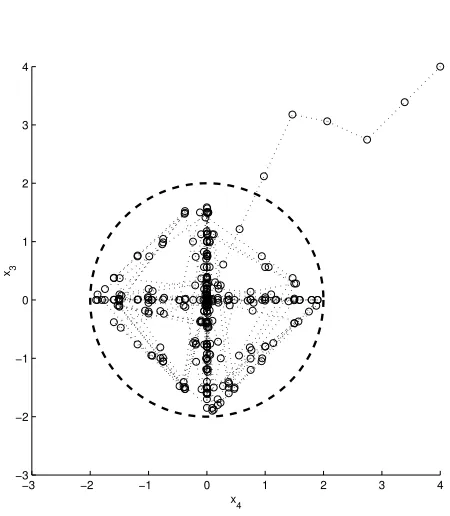
show the projection onto the plane x3-x4 of the simulated state trajectory fork= 12with the new choice ofRw. Again,
starting at point [4 4]T, the trajectory (dotted) is soon
confined within the target set Π ={x∈Rn : k2xTR wx≤
1} described by the dashed ellipsoid centered at zero and with axes 1
k√λ1q1 and
1
k√λ2q2 where q1 = [
1
√
2 1
√
2]
T,
q2 = [−√12 √12]T, λ1 = 1/2 and λ2 = 1 are the eigenvectors and eigenvalues of the submatrix
· 3
4 − 1 4
−1 4
3 4
¸
of Rw. To simulate a worst case scenario in the sense
clarified above, demandw(t)is randomly extracted from the set{w(1), w(2), w(3), w(4)} with uniform probability where
w(1)= [0 ±1 0 0 0]T w(2)= [0 0 ±[2 2] 0]T
w(3)= [0 0 ±[−2√2 2√2] 0]T w(4) = [0 0 0 0 ±1]T.
−3 −2 −1 0 1 2 3 4
−3 −2 −1 0 1 2 3 4
x3
[image:7.612.322.550.52.238.2]x4
Fig. 5. Projection onto the planex3-x4of the simulated state trajectory
fork= 1
2, see Fig. 3 (b). Starting at point[4 4]
T
, the trajectory (dotted) is soon confined within the sphere of radius 3 and centered in the origin.
−3 −2 −1 0 1 2 3 4
−3 −2 −1 0 1 2 3 4
x3
x4
Fig. 6. Projection onto the planex3-x4 of the simulated state trajectory
fork=1
2, whenRwis as in (21). Starting at point[4 4]
T
, the trajectory (dotted) is soon confined within the target set (dashed ellipsoid).
VI. CONCLUSIONS AND FUTURE WORKS
This work is a continuation of [2] and is in line with some recent applications of LMI techniques to inven-tory/manufacturing systems [7]. In a future work, we will study the validity in probability of the LMI conditions derived in this paper. This is in accordance with some recent literature on chance LMI constraints developed in the area of robust optimization [5], [8].
REFERENCES
[1] E. Adida, and G. Perakis. A Robust Optimization Approach to Dynamic Pricing and Inventory Control with no Backorders.
Mathe-matical Programming, Ser. B 107:97–129, 2006.
[2] D. Bauso, F. Blanchini, and R. Pesenti. Robust control policies for multi-inventory systems with average flow constraints. Automatica, Special Issue on Optimal Control Applications to Management Sci-ences, 42(8): 1255–1266, 2006.
[3] D. Bauso, L. Giarr´e and R. Pesenti. Robust control of uncertain multi-inventory systems and consensus problems.Accepted to the 17th IFAC
World Congress, Seoul, Korea, July 2008.
[4] F. Blanchini, F. Rinaldi and W. Ukovich. A network design problem for a distribution system with uncertain demands. SIAM Journal on
Optimization, 7: 560–578, 1997.
[5] A. Ben-Tal, A. Nemirovsky. On tractable approximations of uncertain linear matrix inequalities affected by interval uncertainty. SIAM
Journal on Optimization, 12: 811–833, 2002.
[6] D. Bertsimas, A. Thiele. A Robust Optimization Approach to Inven-tory Theory. Operations Research, 54(1): 150–168, 2006.
[7] E. K. Boukas. Manufacturing Systems: LMI Approach. IEEE
Transactions on Automatic Control, 51(6): 1014-1018, 2006.
[8] G. Calafiore, M. C. Campi. Uncertain Convex Programs: Random-ized Solutions and Confidence Levels. Mathematical Programming, 102: 25–46, 2005.
[9] S.T. McCormick. Submodular containment is hard, even for networks.
[image:7.612.64.289.422.680.2]
![Fig. 3 displays the time plot of the state variable xcomponentwise. With the above choices ofand observe that in all of the three cases, from aboutRt >w(t) 10 on, the state x(t) never exceeds the interval [−k, k] k = 13, 12, 1, and = I, the possible values for P satisfying condition](https://thumb-us.123doks.com/thumbv2/123dok_us/8010541.211785/6.612.91.263.66.202/displays-variable-xcomponentwise-choices-interval-possible-satisfying-condition.webp)