This is a repository copy of
Calculating Errors for Measures Derived From Choice
Modeling Estimates
.
White Rose Research Online URL for this paper:
http://eprints.whiterose.ac.uk/84335/
Version: Accepted Version
Proceedings Paper:
Hess, S and Daly, A (2009) Calculating Errors for Measures Derived From Choice
Modeling Estimates. In: TRB 88th Annual Meeting Compendium of Papers DVD.
Transportation Research Board 88th Annual Meeting, 11-15 Jan 2009, Washington DC.
National Academy of Sciences , ? - ? (23).
Reuse
Unless indicated otherwise, fulltext items are protected by copyright with all rights reserved. The copyright exception in section 29 of the Copyright, Designs and Patents Act 1988 allows the making of a single copy solely for the purpose of non-commercial research or private study within the limits of fair dealing. The publisher or other rights-holder may allow further reproduction and re-use of this version - refer to the White Rose Research Online record for this item. Where records identify the publisher as the copyright holder, users can verify any specific terms of use on the publisher’s website.
Takedown
If you consider content in White Rose Research Online to be in breach of UK law, please notify us by
Calculating errors for measures derived from choice
modelling estimates
Andrew Daly∗ Stephane Hess† Gerard de Jong‡
July 31, 2011
Abstract
The calibration of choice models produces a set of parameter estimates and an associated covariance matrix, usually based on maximum likelihood es-timation. However, in many cases, the values of interest to analysts are in fact functions of these parameters rather than the parameters themselves. It is thus also crucial to have a measure of variance for these derived quan-tities and it is preferable that this can be guaranteed to have the maximum likelihood properties, such as minimum variance. While the calculation of standard errors using the Delta method has been described for a number of such measures in the literature, including the ratio of two parameters, these results are often seen to be approximate calculations and do not claim maximum likelihood properties. In this paper, we show that many measures commonly used in transport studies and elsewhere are themselves maximum likelihood estimates and that the standard errors are thus exact, a point we illustrate for a substantial number of commonly used functions. We also discuss less appropriate methods, notably highlighting the issues with using simulation for obtaining the variance of a function of estimates.
Keywords: discrete choice models; standard errors; parameter significance; delta method; maximum likelihood
1
Introduction
The use of discrete choice models entails the estimation of values for the various parameters used in the model specification, often on the basis of the maximum
∗Institute for Transport Studies, University of Leeds, and RAND Europe, [email protected] †Institute for Transport Studies, University of Leeds, [email protected], Tel: +44 (0)113
34 36611
‡Institute for Transport Studies, University of Leeds, Significance and CTS Stockholm,
likelihood criterion. This criterion has the advantages that it yields minimum-variance, asymptotically unbiased and asymptotically multivariate-normal esti-mates and also gives asymptotic estiesti-mates of the errors associated with those estimates. These error estimates allow analysts to assess the success of their es-timation, using techniques such ast-ratios or (for non-linear models) asymptotic
t-ratios.
Independently of the model structure and utility specification used in a dis-crete choice analysis, the final estimates thus consist of a vector of parameters
β and a covariance matrix Ω. However, in many cases, the values of interest to analysts are in fact not the elements of the vector β itself, but other model outputs based on these estimates.
The calculation of these derived measures as functions of the estimated pa-rameters β is well documented in the existing literature. However, by being functions ofβ, these measures are also subject to the errors associated with the estimation of the parameters. It is important therefore to be able to assess the error associated with statistics derived from the estimated parameters. This has received relatively little attention, and many studies still report derived measures without the associated standard errors.
In many cases, the required statistics are also functions of the data, which may well have measurement error. Calculating the error in statistics caused by data error requires assumptions concerning the data error distribution, which is of a different nature and may be substantially greater than the error caused by estimation error. Consideration of both types of error has been discussed in a small literature; for a review in the context of travel demand see de Jong et al.
(2007). Data error is beyond the scope of this paper, which focusses on estimation error.
Where analysts have made the extra effort to produce standard errors for functions of their parameter estimates, they have often relied on two different approaches, namely simulation of the standard errors, or calculation on the ba-sis of the so-called Delta method. While its use may be attractive in the case of complex functions, simulation of the standard errors can in fact be seriously misleading, as highlighted once more in numerical examples in the present pa-per. The Delta method on the other hand is typically regarded as providing an
approximation to the true standard errors, the quality of which is not usually discussed. The approach of Armstrong et al. (2001) is not widely used, because of its computational complexity, but is a valid alternative.
functions with full maximum likelihood properties.
The remainder of this paper is organised as follows. The following section discusses the nature of standard errors calculated by the Delta method. This is followed by a discussion of a number of regularly used measures in Section 3, showing in each case that the calculated standard errors are indeed exact rather than approximations. Section 4 presents an empirical example for the ratio of coefficients that contrasts the Delta method with simple simulation of the errors; it is indicated that the variance of the simulation estimator does not exist, in line with discussions inDaly et al.(2011). Finally, Section5summarises the findings of the paper.
2
General methodology
This section begins by recalling the basic properties of parameters estimated by maximum likelihood methods and the error measures associated with them. It goes on to discuss the application of functions to obtain derived measures from parameter measures and the Delta method for obtaining estimates of error in derived measures. The second subsection discusses the estimation of errors by sampling, while the third subsection presents the main theorem of the paper, which shows that the transformed estimates are themselves maximum likelihood estimates under quite general conditions and that the Delta method errors are the Cram´er-Rao lower bound of errors. Finally, a general method is described for developing error estimates for new parameter transformations in a multivariate context.
2.1 Parameter estimates and error estimates
It is imagined that our choice model is estimated from a large number N of observations of revealed or stated preferences of individual decision makers1. We
further assume that this model contains a number of unknown parameters which are estimated using the maximum likelihood criterion. Because of this context it is possible in fairly general terms to state the key properties of the parameter estimates.
The classical result that is widely used in this context is that, provided rea-sonable conditions are met and the model is correctly specified, then the expected score (first derivative of the likelihood function with respect to the model param-eters) is zero and the maximum likelihood estimatesβ of the model parameters
1Because we have assumed that there is a large number of observations, we shall not
converge, asN increases, to a normal distribution around the true valuesβ∗:
√
N(β−β∗)→n(0,Ω) (1)
where Ω is a symmetric positive definite matrix.
If the model is correctly specified and the optimum is well defined, then Ω is minus the inverse of the Hessian (matrix of second derivatives) of the likelihood function with respect to the model parameters and forms the Cram´er-Rao lower bound, so these estimates are minimum variance.
If the model is not correctly specified but the expected score of the likelihood function is zero at β∗, or when it is inconvenient to calculate the true second
derivative matrix, other matrices can be substituted, as indicated in the textbooks (e.g.Train,2009). However, in these cases we no longer have maximum likelihood estimates, although the Delta method can still be used as an approximation.
Then let β be a correctly-specified maximum likelihood estimator of a vec-tor β∗ of dimension L and let Ω be the covariance matrix of β around β∗. Let
Φ=Φ(β): RL→RLbe a differentiable function. The interest now lies in
comput-ing standard errors for Φ.
The first point is that if β∗ is the true value of β, then Φ∗ = Φ(β∗) is the
true value of Φ. This depends only on Φ being an ordinary single-valued function (e.g. not a square root, which would leave Φ∗ being defined ambiguously).
The Slutsky Theorem states that continuous functions of consistent estima-tors are consistent estimaestima-tors of the functions. That is, making calculations of functions of model parameters gives results that have at least the reasonable property of consistency. For the Slutsky theorem,β does not have to be a maxi-mum likelihood estimator, but if it is, and under certain other conditions, these results can have substantially more status and correspondingly better properties. It is shown by simple calculus in statistical textbooks that a first-order ap-proximation to the error in Φ induced by the error inβ is given by
cov(Φ) = Φ′TΩΦ′ (2)
where Φ′ is the vector first derivative of the function Φ with respect to β and Ω is the covariance matrix of the estimates of β. Moreover, Greene (2008, pp. 1055-1056) indicates that if β is asymptotically normally distributed, and Φ is continuous (and of course differentiable, though this is not stated byGreene 2008) then Φ is also asymptotically normally distributed.
2.2 Estimation of errors by sampling
In the context of maximum likelihood estimates ofβ, Equation 2can be seen as a two-stage calculation of the variance of the function Φ. First, the matrix Ω is an asymptotic approximation to the true covariance matrix of the estimates
β. Second, the distribution of Φ has commonly been seen as some complicated function derived from the asymptotic normality of the distribution of β. In the case of the estimate of the ratio of two parameters, we might naturally call on literature which describes the distribution of the ratio of two normally distributed random variables: skewed, with complications arising when the denominator gets close to 0.
For example, Armstrong et al. (2001) present an approach to calculating asymptotic t-ratios for parameter ratios based on the asymptotic normality of the numerator and denominator. They also give an alternative approach, calcu-lating likelihood ratios relative to restricted versions of the model, an approach with greater sophistication but not always feasible and, as they concede, often “tedious” in practice.
The approach of making calculations based on the assumption that the nu-merator and denominator of the parameter ratio are normally distributed is also widespread in other literatures such as health economics (see e.g. Hole, 2007). The difficulties of this rigid approach, requiring an exact normal distribution of the estimated parameters (which is only an approximation) and therefore losing sight of the fact that their ratio is equally justifiably normally distributed (see the Greene 2008 result mentioned above) leads to a range of complicated and unsatisfactory approaches, such as sampling from the ‘normal’ distributions of the original parameters and using the samples as arguments for the function, an approach sometimes attributed toKrinsky and Robb(1986,1991), in cases where these complications are not necessary and sometimes incorrect.
2.3 Status of transformed estimates
A deeper understanding of Equation 2 can be obtained along the lines set out by Cramer (1986, Section 3.1). In Section 2.1 we established that providing Φ is differentiable, then the distribution of Φ converges asymptotically to a normal distribution around the true value Φ∗:
√
N(Φ−Φ∗)→n 0,Φ′TΩΦ′
(3)
where Ω is the covariance matrix of β, i.e. Φ is asymptotically equivalent to an MLE of Φ∗, as it has the same asymptotic distribution.
It may be tempting to claim that Φ can be regarded as an MLE with no further ado, that it represents the maximisation of likelihood over a space induced by the transformation Φ. Cramer(1986), however, prefers the more widely accepted view, which is to consider the reparametrisation of the model by an invertible vector function to obtain a vector η with the same dimension as β:
η=g(β) andβ =g−1(η) (4)
For the transformation g to be invertible it must be one-to-one2, as well as dif-ferentiable. While these conditions may be restrictive from a mathematical point of view, in practice many important functions can be shown to have the required properties. With these conditions, Cramer shows that the properties of the de-pendent variable are not affected by the transformation, so that η =g(β) is an MLE ofη∗. Cramerthen goes on to derive the covariance of Φ around Φ∗ as:
cov(Φ) =g′TΩg′ (5)
whereg′ is the derivative matrix (Jacobian) ofgwith respect toβ. This is exactly
the result from Equation2, but now, because we know η to be an MLE, we also know that cov(Φ) is the Cram´er-Rao lower bound of minimum variance for the estimator.
The approach of Cramercan be summarised in the following theorem.
Theorem: Let β be a correctly-specified maximum likelihood estimator of a
vectorβ∗ of dimensionLand let Ω be the covariance matrix ofβ aroundβ∗. Let
Φ: RL→RL be a differentiable and invertible function. Then:
1. Φ∗ = Φ(β∗) is the true value of Φ(β∗);
2. Φ = Φ(β) is a maximum likelihood estimator of Φ∗; and
3. the covariance matrix of Φ around Φ∗ attains the Cram´er-Rao lower bound
and is given by:
cov(Φ) = Φ′TΩΦ′, (6)
where Φ′ is the first derivative matrix of Φ.
We are now in a position to reassess the results derived by the Delta Method. Instead of seeing this approach as being a general way to develop useful ap-proximations for the error in functions of parameters, we can now see that the functions of parameters can themselves be interpreted as true maximum likeli-hood estimates, while the Delta Method is exactly what is required to obtain the
true Cram´er-Rao covariance of the transformed parameter estimates around the true values.
The Theorem gives us two principal benefits. First, it generalises a number of results that have been derived as approximate calculations. Second, it gives a new status to the transformed parameters Φ(β).
Consider the important example of estimating the ratio of two estimated pa-rameters. By considering the parameters to be maximum likelihood estimators and therefore asymptotically normally distributed about the true value, a Taylor expansion can be used to approximate the distribution and thus derive the vari-ance. Given the theorem above, however, it is not necessary to make approximate calculations based on Taylor expansions but a direct statement of the result can be given, based on the first derivatives. Furthermore, the result indicates that the parameter ratio is itself a maximum likelihood estimate and is therefore itself consistent, unbiased and normally distributed around the true ratio. The vari-ance has the same value as given by the textbook formula, but the result shows that this is in fact the true Cram´er-Rao lower bound, rather than an approximate value.
It may also be noted from Cramer (1986) that if the theorem does not hold because Φ is not invertible, then Φ is still asymptotically equivalent to a maximum likelihood estimator. The use of Φ is unlikely to lead to false conclusions.
2.4 A general approach
Similar reasoning can be applied for any subset of the estimates. Of course, the transformations being applied must remain invertible and differentiable.
Thus, Φ in the above notation may contain a large number of functions of
β while we may only be interested in a single function. Here, we could have that Φk gives a single function of a specific subset of parameters of β, say βΦk
with covariance matrix ΩΦk. Providing that the function defined by changing
βk to this Φk, leaving all the otherβ values unchanged, satisfies the conditions
of the theorem, in particular that it is invertible, then we can make the claims of the Theorem for Φk. In the remainder of this paper, we will assume that Φ
relates to a single function of a subset of the parameters and will drop subscripts accordingly. We are then interested in the variances of an individual function Φ rather than the covariance matrix of a set of functions.
The transformations that satisfy the requirements of the Theorem are then those that convert a single variable to another single variable by a differentiable and invertible function. All of the functions we shall consider are differentiable and these functions are invertible if the derivative does not change sign or become zero, because they are continuous and strictly monotonic. That is, we can apply the Theorem if the derivative of Φ with respect to one β parameter does not change sign as β changes.
Before proceeding, we will introduce a formulation that facilitates the calcu-lation when dealing with a single Φ and a large number of parameters β. As shown above, we have that var(Φ) = Φ′TΩΦ′. Here, Φ′ hasL elements, namely
the derivative of Φ with respect to each of theL elements inβ. Furthermore, Ω hasL2 elements, of which only L2+L
2 are unique, since the matrix is symmetric.
Denoting the individual elements in Φ′ and Ω asφ′
landωlmrespectively, we have
that:
var(Φ) = Φ′TΩΦ′ =
L X
l=1
φ′l L X
m=1
φ′mωml !
, (7)
where it can be further seen that this is equal to:
var(Φ) =
L X
l=1
φ′l2ωll+ 2 L X
l=2
l−1
X
m=1
φ′lφ′mωlm, (8)
3
Standard errors for commonly used measures
This section presents formulae for the variances of a number of measures com-monly used in transport analysis and elsewhere, obtained using the approach described in the previous section. Specifically, we look at different specifications of Ω (β), whereβ is a vector grouping together all estimated parameters, with Ω being the covariance matrix of the vectorβ, with individual elements defined as
ωkl. Each time, we discuss how the obtained variances can be shown to have the
same MLE properties as the coefficients from which they are obtained.
Table 1 summarises the calculations needed to obtain the variances for four basic but widely used measures, namely the sum and difference of two parameters, and the ratio and product of two parameters. We also show the variance for the reciprocal ofβ1, which implies that the t-ratio of the reciprocal ofβ1 with respect
to zero is exactly the same as the t-ratio ofβ1 with respect to zero, namely √βω1
11,
i.e. β1 divided by its standard error. Alongside the variance for the product of
two estimators, we also see that the variance of the square of an estimator is given by the variance of the estimator multiplied by four times the square of the estimator; thet-ratio for the square of a parameter is thus half the t-ratio for the parameter itself, a result that is useful when moving between standard deviations and variances for random coefficients. Finally, Table 1 also shows the variances for ratios of parameters (e.g. willingness-to-pay indicators, WTP) in the case of non-linear utility functions, in particular when a Box-Cox transform is used.
We now turn to the issue of invertibility, and by extension the maximum likelihood properties of these error measures. As can be seen from the fifth column in Table 1, the signs of the partial derivatives of Φ are either fixed or independent of the relevant parameter (i.e. the parameter which we differentiate against), with the exception of the square, i.e. Φ = β2
1. Here, if the sign of β
is known, as will generally be the case, the derivative has a fixed sign. As a conclusion, we can state the standard errors obtained using the Delta method for the various measures in Table1 are exact3.
We now move to a discussion of model-specific quantities of interest. Specifi-cally, in advanced models, the behaviour is quantified by a number of parameters that impose a certain structure on the error term. This includes the correlation between error terms in Generalised Extreme Value (GEV) models (cf. McFad-den, 1978) as well as the parameters used for the distributions of preferences in random coefficients models. However, the actual measures of interest are often again a function of these parameters rather than the parameters themselves,
lead-3A further case that deserves special attention is with the WTP in the presence of a Box-Cox
Table 1: Standard errors for commonly used measures
Function Φ β∗ φ′
k= ∂Ω
∂β∗ Sign ofφ′k var(Φ) Limitations
Sum β1+β2 β1 φ
′
1= 1 positive ω
11+ω22+ 2ω12 None
β2 φ′2= 1 positive
Difference β1−β2 β1 φ
′
1= 1 positive ω
11+ω22−2ω12 None
β2 φ′2=−1 negative
Ratio β1
β2
β1 φ′1= β12 sign ofβ2
β 1 β2 2 ω11 β2 1 + ω22 β2 2 −2
ω12
β1β2
β26= 0
β2 φ′2=− β1
β2
2 minus sign ofβ1
Inverse β11 β1 φ′1=−β12
1 negative
ω11
β4
1 β16= 0
Product β1β2 β1 φ
′
1=β2 sign ofβ2 β2
2ω11+β21ω22+ 2β1β2ω12 None
β2 φ′2=β1 sign ofβ1
Square β2
1 β1 φ′1= 2β1 sign ofβ1 4β12ω11 None
WTP with Box-Cox transform β1 β2
xλ1−1 1
xλ2−1 2
β1 φ′1=β12
xλ1−1 1
xλ2−1 2
sign ofβ2
use Equation8 x1>0, x2>0
λ1 φ′2= β1
β2
xλ1−1 1 ln(x1)
xλ2−1 2
sign of β1ln(x1)
β2
β2 φ′3=− β1
β2 2
xλ1−1 1
xλ2−1 2
minus sign ofβ1
λ2 φ′4=− β1
β2
xλ1−1 1 x
λ2−1 2 ln(x2)
x2λ2−2 2
minus sign of
β1ln(x2)
β2
ing to a requirement for the calculation of appropriate error measures. Table 2
summarises the calculation of variances for a number of such measures.
We first look at the correlation between error terms in a two-level Nested Logit (NL) model as a function of the structural parameter λ, and an approximation to the correlation between the errors for two alternatives iand j in a two-level Cross-Nested Logit (CNL) model, with K nests, where αj,k is the allocation
parameter for alternative j and nest k (cf. Papola, 2004;Marzano and Papola,
2008). For both measures, the fifth column shows no problems with invertibility as the signs of the partial derivatives are fixed, hence ensuring that the standard errors obtained with the Delta method are exact.
Researchers and practitioners are increasingly relying on the Mixed Multino-mial Logit (MMNL) model to represent random variations in the marginal utili-ties across respondents. From an interpretation point of view, we are interested in the moments of the estimated distribution, but, in contrast to the commonly used Normal distribution, these moments in other distributions do not generally equate to the estimated parameters. Table 2shows the calculations for the vari-ances for the means and standard deviations for two commonly used alternatives to the Normal, namely the Triangular distribution4 and the Lognormal
distribu-tion5. Corresponding variances for the estimated variance can be obtained with the help of the formula for squares in Table 1. Invertibility and hence exactness of the standard errors obtained with the Delta method is clearly ensured for all of these measures except for the standard deviation of the Triangular distribu-tion, where problems arise for the mode, i.e. c. If, as is commonly the case, a symmetrical Triangular is used, we simply have thatc= a+b
2 , so that no problem
arises. If an asymmetrical Triangular is used, invertibility is guaranteed (i.e. the variances are still exact) if we assume that the sign of the skewness is known.
While most MMNL applications still make use of independently distributed random coefficients, it has been recognised that it is important to also allow for correlation between the coefficients. In the rare cases where a multivariate distribution is actually used, this is almost exclusively based on a multivariate Normal (MVN) distribution. The estimation of a multivariate Normal produces estimates of the mean coefficient values along with the Cholesky matrix Λ, on the basis of which it is possible to calculate covariance and correlation measures. The outputs of interest in this context are the lower triangular Cholesky matrix
4Witha,b and cgiving the lower boundary, upper boundary and mode of the Triangular
distribution.
5With the mean and standard deviation of the underlying Normal distribution being given
Table 2: Standard errors for model specific measures
Function Φ β∗ φ′
k= ∂β∂Ω∗ Sign ofφ′k var(Φ) Limitations
NL correlation 1−λ2 λ φ′
1=−2λ negative 4λ2ω2λ 0< λ≤1
CNL correlation PK k=1α
1 2 i,kα 1 2 j,k 1−λ2k
λk, k= 1, .., K φ′l=−2λlα
1 2
i,lα
1 2
j,l,1≤l≤K negative
use Eq.8
0≤λk≤1,∀k
αi,k, k= 1, .., K φ′l= 12α
−12
i,l α
1 2
j,l
1−λ2l, K < l≤2K positive 0≤αi,k≤1,∀k,Pkαi,k=
αj,k, k= 1, .., K φ′l=12α
−12
j,l α
1 2
i,l
1−λ2l,2K < l≤3K positive 0≤αj,k≤1,∀k,Pkαj,k=
Mean of
Triangular µT =a+3b+c
a φ′
1=13 positive ω
11 +ω22 +ω33 +2ω12 +2ω13 +2ω23
9 a≤c≤b
b φ′
2=13 positive
c φ′
3=13 positive
SD of Triangular σTq =
a2 +b2 +c2−ab−ac−bc
18
a φ′
1=2a18−σTb−c negative
(2a−b−c)((2a−b−c)ω11 +(2b−a−c)ω12 +(2c−a−b)ω13 ) 182σ2T
a≤c≤b
b φ′
2=2b18−σTa−c positive +
(2b−a−c)((2b−a−c)ω22 +(2c−a−b)ω23 ) 182σ2
T
c φ′
3=218c−σTa−b sign of 2c−a−b +
(2c−a−b)2ω33 182σ2T
Mean of
Lognormal µLN=eµN+ σ2N
2
µN φ′1=eµN +σ
2
N
2 =µLN positive (µLN) µ2
LN
ω11+σN2ω22+ 2ω12σN
σN>0 σN φ′2=σNeµN+
σ2N
2 =σNµLN positive (µLN)
SD of LognormalσLN=
q
e2µN+2σ2N−e2µN+σ2N
µN φ′1= 2e 2µN+2σ2N
−2e2µN+σN2
2 r
e2µN+2σ
2
N−e2µN+σ
2
N
=σLN positive σLN2 ω11+ 2σN
e2µN+2σ2N+σ2LN
w12 σ
N≥0
σN φ′2=σN e
2µN+2σ2N σLN +σLN
!
positive +σ2N e2µN+2σ
2
N σLN +σLN
!2
ω22
Variance in MVN ΦA(a) =Pak=1 sa,k
2 s
a,k, a≥k φ′A,a,k= 2sa,k see text use Eq.8 a≥k
Covariance in
MVN ΦB(a, b) =Pak=1sa,ksb,k sa,k, a≥k φ
′
B,a,k=sb,k see text use Eq.8 k≤a < b
sb,k, b≥k φ′B,b,k=sa,k
Correlation in
MVN ΦC(a, b) =
ΦB(a,b)
√Φ
A(a)ΦA(b) sj,k, j≥k
φ′
C,j,k= φ′
B,j,k(a,b) √Φ
A(a)ΦA(b) see text use Eq.8 j≥k, a < b −ΦB(a,b)
φ′
A,j,k(a)ΦA(b)+φ′A,j,k(b)ΦA(a)
2(ΦA(a)ΦA(b))32
Λ, given by:
Λ =
s1,1 0 0 . . . 0
s2,1 s2,2 0 . . . 0
..
. ... ... ... ...
sK,1 sK,2 sK,3 . . . sK,K
, (9)
with corresponding covariance matrix of the estimates ΩΛwhere this is a subset of
the covariance matrix for all estimated parameters Ω, and where Λ can be written in vector form as Λ = (s1,1, s2,1, s2,2, . . . , sK,K). We have that the covariance
matrix of the multivariate Normal distribution is now given by ΛTΛ. Table 2
shows the calculations required to obtain variances for three main measures that can be obtained from his, namely the variance of individual coefficients and the covariance and correlation between pairs of coefficients. For the actual calculation of the standard errors, it can be seen that Λ hasPK
k=1kelements, with the same
being the case forφ′A,j,k(a),φB,j,k′ (a, b), andφ′C,j,k(a, b). The covariance matrix
of Λ, ΩΛ has
PK
k=1k
2
elements (PK k=1kby
PK
k=1k), and the variances of the
measures can be obtained straightforwardly by applying Equation8to the partial derivatives.
We know that invertibility is ensured for the covariance in multivariate Nor-mals as the Cholesky decomposition is unique, so that as a result, the standard errors for variances and covariances obtained with the Delta method are exact. By the same reasoning, the correlation transformation is also invertible, given the standard errors.
4
Empirical example
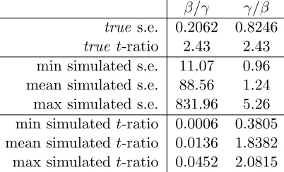
As a final step, we present a simple comparison between the Delta method and simulation, with a view to highlighting the inadequacy of simulation in this con-text. Here, we limit ourselves to the most basic meaningful example, namely the ratio between two coefficients, β and γ. Extensions to more complex situations are straightforward. Our example uses values of −0.05 for β and −0.1 for γ, where we use variances of 0.0001 and 0.0009 respectively, with a covariance of
−0.0001. This gives t-ratios of −5 and −3.33 for β and γ, with a correlation of
−0.33 between the two coefficients. We thus have that βγ = 0.5 and γβ = 2. Using the appropriate formulae from Table 1, we obtain standard errors for these two ratios of 0.2062 and 0.8246 respectively, giving t-ratios of 2.43 for both βγ and
γ
β; from Table 1, it can be see that the t-ratio against zero for the inverse of a
Table 3: Empirical example: standard errors for a ratio of two coefficients, statis-tics over 50 runs, each with 107 draws
β/γ γ/β
true s.e. 0.2062 0.8246
true t-ratio 2.43 2.43 min simulated s.e. 11.07 0.96 mean simulated s.e. 88.56 1.24 max simulated s.e. 831.96 5.26 min simulated t-ratio 0.0006 0.3805 mean simulated t-ratio 0.0136 1.8382 max simulatedt-ratio 0.0452 2.0815
As an alternative to using the exact formulae, some analysts may rely on simulation, especially in the case of complex measures where formulae have not been discussed in detail prior to this paper. To illustrate the shortcomings of this approach, simulation was used to try to produce standard errors for βγ and
γ
β in this example. In fact, for a ratio of random normal variables, the variance
does not exist, as is shown byDaly et al.(2011). Although that paper deals with the different context of distribution in the population rather than errors, the mathematics of the ratio of two normally distributed variables is the same, and the literature reviewed and results of the paper show that none of the moments of these ratios exist. However, the simulation approach is sometimes used in practice and it is illuminating to try an extensive simulation to show how that works out. Specifically, we used fifty runs with 107 (ten million) draws forβ and
γ6.
The results of this application are summarised in Table3, giving statistics for the simulated standard errors and the resultingt-ratios for the ratios βγ and γβ7.
Several observations can be made. Firstly, there is a lack of stability across the fifty runs, again highlighting an issue with simulation which depends on the draws used in a specific run, even when making use of 107 draws! We can further see
that the simulation overestimates the true standard error for βγ by over 5,000% in thebest run, and by over 400,000% in theworst run. For γβ, the problems are slightly less pronounced, which is a result of a highert-ratio for the denominator,
6With appropriate consideration of the covariance.
7Theset-ratios are based on the estimates rather than simulated values for the ratios β γ and γ
reducing the chances of values close to zero in the denominator for the second ratio. But even here, thebest run overestimates the standard error by over 15%, while the worst run overestimates it by over 500%. With these problems, it should come as no surprise that thet-ratios are also severely biased, and are not the same for the two ratios as they should be.
It is important to be clear that the simulation results for this ratio are always incorrect. The discussions inDaly et al.(2011) show that all simulations of this ratio give undefined results. In this sense, the simulations ofβγ are less concerning, as the risk of accepting them as valid is small. For γβ, however, there is a clear danger that results in this range could be accepted as valid.
Simulation can be used, of course, in cases when the result that is required actually exists. For a ratio, percentiles may be used. However, in most simple cases it is easier and, as we have shown, more exact, to use the Delta calculation. In more complicated situations (cf.de Jong et al.,2007), simulation is still needed.
5
Discussion and conclusions
5.1 Discussion: t ratios
We close the paper by looking at the consequences that the discussions above have for our interpretation of estimates and their significance. In particular the interpretation of t-ratios and confidence limits requires a little thought.
Earlier, we showed that thet-ratio of the estimate of a reciprocal of an MLE parameter was equal to thet-ratio of the parameter itself. We also showed that the estimate of the reciprocal has just as much status as the initial estimate. Does this mean that a test that a parameter is significantly different from 0 is exactly the same as a test that it is significantly different from infinity? Moreover, how can it be that a parameter estimate and an estimate of the reciprocal of the parameter are both distributed asymptotically normal?
The information on the likelihood function comes out of the estimation pro-cess. At the optimum, we know that the first derivative of the function is zero and we have an estimate (from one or other matrix) of the second derivatives. All of the usual information on errors,t-ratios and confidence limits comes from this matrix of second derivatives.
are exceptions. It is therefore not surprising that we find paradoxes such as thet -ratio of a parameter and its inverse being equal. At the optimum value, we know that the estimate, the first and second derivatives are all consistent between the parameter and its inverse. But as soon as we move away from the optimum, there is no guarantee at all, and it is clear that the likelihood function defined in terms of one or both of the formulations (parameter or inverse) must fail to be quadratic. It is frequently stated that thet-ratios given for non-linear models are approximate. The extent of this approximation is perhaps often underestimated. Is there a better approach? The conventional calculations made for models estimated on the maximum likelihood criterion appear to make best use of the information available at the optimum likelihood value. To get better information, it would be necessary to investigate the true variation of the likelihood function as we move away from the optimum. For example, to obtain 95% confidence limits for a parameter, it would be useful to find the upper and lower values beyond which 2.5% of the likelihood lies, the approach ofArmstrong et al.(2001). These would not necessarily be symmetric around the optimum values of the parameter, but their inverses would represent the upper and lower confidence limits of the inverse of the parameter. One could then test whether any particular value, e.g. 0, lay within the 95% confidence bands. Making these calculations would be time-consuming, as specialised software does not appear to exist and in most cases, therefore, it is necessary to continue to use t-ratios.
5.2 Conclusions
In this paper, we have discussed the issue of computing standard errors for mea-sures that are functions of parameters estimated from discrete choice models. This is an issue of crucial importance as, in choice modelling, the values of in-terest to analysts are in fact often functions of these parameters rather than the parameters themselves. The paper has shown how the simple Delta formula can be used to derive such standard errors while maintaining desirable properties for the standard errors, where, previously, analysts have seen this as an approximate approach.
The paper then presents formulae for the standard errors of a number of regularly used measures, going beyond what is currently available in the choice modelling literature8, and illustrates how they are indeed exact calculations.
The simple example in Section 4 highlights the benefit of this approach over simple simulation;Daly et al.(2011) show that simple simulation must ultimately fail for the important example of a coefficient ratio.
8To allow readers to exploit the formulae developed in this paper, freeware software is being
Future work should extend the set of functions developed in this paper. In this context, given the results of the simulation and the non-existence proof for the variance of the ratio estimator, and the fact that simulation may in the short term remain necessary for some of the most complicated functions, further investigation should be undertaken to determine whether the common practice of estimating errors by simulation is likely to yield serious misinterpretations in other cases as well. The analytical results are clearly more reliable and hence preferable if they can be calculated without undue complication.
Acknowledgements
The authors are grateful to Chandra Bhat and three anonymous referees for extensive comments on earlier versions of the paper. The second author acknowl-edges the financial support of the Leverhulme Trust in the form of aLeverhulme Early Career Fellowship.
References
Armstrong, P., Garrido, R. A., Ort´uzar, J. de D., 2001. Confidence interval to bound the value of time. Transportation Research Part E 37 (1), 143–161.
Cramer, J. S., 1986. Econometric applications of Maximum Likelihood methods. Cambridge University Press, Cambridge.
Daly, A., Hess, S., Train, K., 2011. Assuring finite moments for willingness to pay estimates from random coefficients models. Transportation, forthcoming.
Daly, A., Zachary, S., 1975. Commuters’ values of time. Local Government O.R. Unit Report T55, Reading, UK.
de Jong, G., Daly, A., Pieters, M., Miller, S., Plasmeijer, R., Hofman, F., 2007. Uncertainty in traffic forecasts: literature review and new results for the nether-lands. Transportation 34 (4), 375–395.
Greene, W. H., 2008. Econometric Analysis (Sixth Edition). Pearson Education Inc, Upper Saddle River, NJ.
Hole, A. R., 2007. A comparison of approaches to estimating confidence intervals for willingness to pay measures. Health Economics 16 (8), 827–840.
Krinsky, I., Robb, A., 1991. On approximating the statistical properties of elas-ticities: a correction. Review of Economics and Statistics 72 (1), 189–190.
Marzano, V., Papola, A., 2008. On the covariance structure of the cross-nested logit model. Transportation Research Part B 42 (2), 83–98.
McFadden, D., 1978. Modelling the choice of residential location. In: Karlqvist, A., Lundqvist, L., Snickars, F., Weibull, J. W. (Eds.), Spatial Interaction The-ory and Planning Models. North Holland, Amsterdam, Ch. 25, pp. 75–96.
Papola, A., 2004. Some developments on the cross-nested Logit model. Trans-portation Research Part B 38 (9), 833–854.