University of Southern Queensland
Faculty of Engineering & Surveying
PID Controller Optimisation Using Genetic Algorithms
A dissertation submitted by
Matthew Robert Mackenzie
in fulfilment of the requirements of
ENG4112 Research Project
towards the degree of
Bachelor of Engineering (Computer Systems)
Abstract
Genetic Algorithms are a series of steps for solving an optimisation problem using
genetics as the model (Chambers, 1995). More specifically, Genetic Algorithms use the
concept of Natural Selection – or survival of the fittest – to help guide the selection of
candidate solutions. This project is a software design-and-code project with the aim
being to use MATLAB® to develop a software application to optimise a
Proportional-Integral-Derivative (PID) Controller using a purpose built Genetic Algorithm as the
basis of the optimisation routine. The project then aims to extend the program and
interface the Genetic Algorithm optimisation routine with an existing rotary-wing
control model using MATLAB®.
A systems approach to software development will be used as the overall
framework to guide the software development process consisting of the five main
phases of Analysis, Design, Development, Test and Evaluation.
The project was only partially successful. The Genetic Algorithm did produce
reasonably optimal values for the PID parameters; however, the processing time
required was prohibitively long. Additionally, the project was unsuccessful in
interfacing the optimised controller to the existing rotary-wing model due difficulty in
conversion between SIMULINK® and MATLAB® formats. Further work to apply code
optimisation techniques could see significant reduction in processing times allowing
more iterations of the program to execute thereby achieving more accurate results.
Thus the project results suggest that the use of Genetic Algorithms as an
optimisation method is best suited to complex systems where classical optimisation
University of Southern Queensland
Faculty of Engineering and Surveying
ENG4111/2 Research Project
Limitations of Use
The Council of the University of Southern Queensland, its Faculty of Engineering
and Surveying, and the staff of the University of Southern Queensland, do not accept
any responsibility for the truth, accuracy or completeness of material contained within
or associated with this dissertation.
Persons using all or any part of this material do so at their own risk, and not at the
risk of the Council of the University of Southern Queensland, its Faculty of Engineering
and Surveying or the staff of the University of Southern Queensland.
This dissertation reports an educational exercise and has no purpose or validity
beyond this exercise. The sole purpose of the course pair entitled ``Research Project'' is
to contribute to the overall education within the student's chosen degree program.
This document, the associated hardware, software, drawings, and other material
set out in the associated appendices should not be used for any other purpose: if they
are so used, it is entirely at the risk of the user.
Prof F Bullen
Dean
Certification
I certify that the ideas, designs and experimental work, results, analyses and conclusions
set out in this dissertation are entirely my own effort, except where otherwise indicated
and acknowledged.
I further certify that the work is original and has not been previously submitted for
assessment in any other course or institution, except where specifically stated.
Matthew Robert Mackenzie
Student Number: 001323707
Signature
Acknowledgements
I would like to thank my supervisor Paul for guiding me through this challenge.
I would also like to thank my wife Sandra whose patience has allowed us to balance this
project, work and our young family.
My love to my wife Sandra, my eldest son Joseph and my youngest son Alec.
Matthew Mackenzie
University of Southern Queensland
Contents
Abstract...ii
Certification ... iv
Acknowledgements... v
Contents ... vi
List of Figures... x
List of Tables ...xii
Glossary of Genetic Terms ...xiii
Chapter 1 Introduction... 1
1.1 Project Description... 1
1.2 Aims and Objectives ... 2
1.3 Dissertation Overview ... 3
1.4 Background Literature Review ... 4
1.4.1 Existing Research Emphasis... 5
1.4.2 Future Research Areas... 7
1.4.3 Literature Review Summary... 7
1.5 Project Methodology... 8
1.5.1 Systems Approach to Software Development... 8
1.5.2 Programming Models ... 9
1.5.3 Test Program ... 9
1.5.4 Evaluation and Extension ... 10
1.6 Summary ... 10
Chapter 2 Optimisation ... 12
2.1 Introduction... 12
2.3 Root Finding ... 13
2.4 Categories of Optimisation ... 14
2.5 Natural Optimisation Methods... 15
2.6 Summary ... 16
Chapter 3 Digital Controllers ... 17
3.1 Introduction... 17
3.2 Control System Overview... 18
3.2.1 Analogue Controller ... 18
3.2.2 Computer Controller... 19
3.2.3 Controllers ... 20
3.3 Tuning ... 22
3.4 Summary ... 24
Chapter 4 Genetic Algorithms ... 25
4.1 Introduction... 25
4.2 Biological Genetic Optimisation... 25
4.3 Genetic Algorithms ... 27
4.4 Advantages and Disadvantages... 27
4.5 Genetic Algorithm Process ... 28
4.5.1 Problem Definition and Encoding ... 28
4.5.2 Initialisation... 29
4.5.3 Decoding... 29
4.5.4 Cost... 30
4.5.5 Selection ... 30
4.5.6 Mating... 31
4.5.7 Mutation ... 32
4.5.8 Convergence ... 32
4.6 Summary ... 33
Chapter 5 Argo... 35
5.1 Introduction... 35
5.2 Definition ... 35
5.3 Encoding ... 36
5.4 Argo Genetic Algorithm ... 37
5.6.2 CostSecond ... 41
5.6.3 CostFirstRandomDelay ... 42
5.7 Natural Selection... 42
5.7.1 Tournament Selection... 42
5.7.2 Roulette Wheel ... 43
5.8 Mating ... 43
5.9 Mutation... 44
5.10 Convergence ... 44
5.11 Argo Input And Control GUI ... 46
5.12 Summary ... 46
Chapter 6 Testing & Analysis Of Results ... 48
6.1 Introduction... 48
6.2 Basic Argo Operation... 49
6.2.1 First Order Test Control System... 49
6.2.2 Second Order Test Control System ... 49
6.2.3 Conduct of Base Performance Testing ... 50
6.2.3.1 Base Performance Testing – Phase A ... 50
6.2.3.1.1 Base Performance Testing – Test A1... 51
6.2.3.1.2 Base Performance Testing – Test A2... 52
6.2.3.1.3 Base Performance Testing – Test A3... 54
6.2.3.1.4 Base Performance Testing – Test A4... 55
6.2.3.1.5 Base Performance Testing – Test A5... 56
6.2.3.2 Base Performance Testing – Phase B ... 58
6.2.3.3 Base Performance Testing – Phase C ... 60
6.2.3.4 Base Performance Testing – Phase D ... 61
6.3 Advanced Argo Operation ... 61
6.3.1 Conduct of Advanced Performance Testing... 61
6.3.1.1 Advanced Performance Testing – Phase E ... 62
6.3.1.2 Advanced Performance Testing – Phase F ... 64
6.3.1.3 Advanced Performance Testing – Phase G ... 64
6.3.2 Other Test Observations ... 68
6.4 Summary ... 69
6.4.1 Base Performance Testing Results ... 69
6.4.2 Advanced Performance Testing Results... 70
7.1 Dissertation Summary... 71
7.2 Basic Argo Operation... 72
7.2.1 Accuracy... 72
7.2.2 Processing Time ... 72
7.2.3 Basic Parameters ... 73
7.3 Advanced Argo Operation ... 74
7.3.1 Roulette Wheel Selection ... 74
7.3.2 Rotary-Wing Control Model Simulation... 74
7.4 Further Work... 74
List of References ... 76
Bibliography ... 78
Appendix A Project Specification...A-1
Appendix B MATLAB® Source Code – Argo ... B-1
Annex A to Appendix B Argo – Main Routine... B-3
Annex B to Appendix B Argo – Genetic Algorithm Random Delay ... B-6
Annex C to Appendix B Argo – InitialisePopulation... B-11
Annex D to Appendix B Argo – TournamentSelection ... B-13
Annex E to Appendix B Argo – ParseBits ... B-15
Annex F to Appendix B Argo – RouletteWheel... B-17
Annex G to Appendix B Argo – Mutate... B-19
Annex H to Appendix B Argo – Crossover... B-21
Annex I to Appendix B Argo – CalcFitnessRandomDelay... B-24
Annex J to Appendix B Argo – CostFirst... B-25
Annex K to Appendix B Argo – CostFirstRandomDelay ... B-27
Annex L to Appendix B Argo – CostSecond ... B-29
Annex M to Appendix B Argo – ARGOGUI... B-31
Appendix C Cost Functions ...C-1
C.1 First Order System ... C-2
C.2 Second Order System... C-7
List of Figures
Figure 1-1 Systems Approach... 9
Figure 2-1 Optimisation Model... 13
Figure 3-1 Analogue Control System (based on (ELE3105 2007, mod. 1, fig. 1.1) ) .... 18
Figure 3-2 Computer Controlled System (based on (ELE3l05 2007, mod. 5, fig. 5.1) ) 19 Figure 3-3 Digital Control Loop (based on (Leis 2003, mod. 1; mod.4) ) ... 21
Figure 3-4 Adaptive Digital Control System ... 23
Figure 4-1 Biological Genetic Algorithm Process Flow... 29
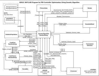
Figure 5-1 Argo Genetic Algorithm... 38
Figure 5-2 Data Flow Diagram ... 39
Figure 5-3 Initialization Function Algorithm... 39
Figure 5-4 Tournament Selection Algorithm... 42
Figure 5-5 Roulette Wheel Selection Algorithm ... 43
Figure 5-6 Crossover Algorithm ... 44
Figure 5-7 Mutation Algorithm... 44
Figure 5-8 Convergence Testing... 46
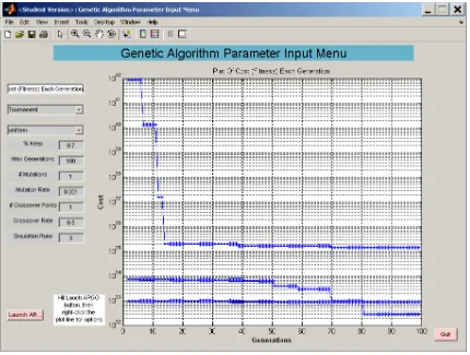
Figure 5-9 Argo Input and Control GUI ... 46
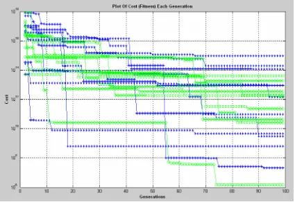
Figure 6-1 Semi-Log Cost Plot Varying Crossover Points... 51
Figure 6-2 Semi-Log Cost Plot Varying Distribution... 53
Figure 6-3 Semi-Log Cost Plot Varying NKeep... 54
Figure 6-4 Semi-Log Cost Plot Varying Crossover Rate... 55
Figure 6-5 Semi-Log Cost Plot Varying Mutation Rate ... 57
Figure 6-6 Semi-Log Cost Plot After 100,000 Generations ... 58
Figure 6-7 Semi-Log Cost Plot After 10000 Generations ... 59
Figure 6-8 Semi-log Cost Plot Varying Selection Method ... 63
Figure 6-9 Error Response From First Order System With Varying Time Delayed Inputs... 65
Figure 6-11 Semi-Log Cost Plot Varying Delayed Input Mean ... 67
Figure C -1 Optimum Response (Steady State Error) for the First Order Test Control System with a PID Controller with Delayed Start and Unit Step Input... C-6
Figure C -2 Optimum Response (Output) for the First Order Test Control System with a PID Controller with Delayed Start and Unit Step Input ... C-6
Figure C -3 Optimum Response (Steady State Error) for the Second Order Test Control System with a PID Controller and Unit Ramp Input ... C-9
List of Tables
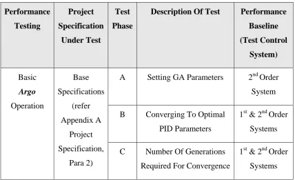
Table 6-1 Test Plan ... 48
Table 6-2 Legend for Figure 6-1... 52
Table 6-3 Legend for Figure 6-2... 53
Table 6-4 Legend for Figure 6-3... 54
Table 6-5 Legend for Figure 6-4... 55
Table 6-6 Legend for Figure 6-5... 57
Table 6-7 Results for Phase C Base Performance Testing (First Order Test System).... 58
Table 6-8 Results for Phase C Base Performance Testing (Second Order Test System)59 Table 6-9 Argo Execution Times... 61
Table 6-10 Legend for Figure 6-8... 63
Table 6-11 Legend for Figure 6-11... 67
Glossary of Genetic Terms
Allele 1. The American Heritage® Dictionary (2004) defines an
allele as “one member of a pair or series of genes that
occupy a specific position on a specific chromosome.”
Chromosome 1. The American Heritage® Stedman's Medical Dictionary
(2006) defines a chromosome as “a threadlike linear
strand of DNA and associated proteins in the nucleus of
eukaryotic cells that carries the genes and functions in the
transmission of hereditary information.”
Gene 2. The American Heritage® Stedman's Medical Dictionary
(2006) defines gene as “a hereditary unit that occupies a
specific location on a chromosome, determines a
particular characteristic in an organism by directing the
formation of a specific protein, and is capable of
replicating itself at each cell division.”
3. The American Heritage® Dictionary (2004) defines a
gene as “a hereditary unit consisting of a sequence of
DNA that occupies a specific location on a chromosome
and determines a particular characteristic in an organism.
Genes undergo mutation when their DNA sequence
Genetic Algorithm 4. Whitley (n.d.) defines Genetic Algorithms as “a family of
computational models inspired by evolution” which are
also “population-based models that uses selection and
recombination operators to generate new sample points in
a search space.”
5. Cantu-Paz (2001) defines Genetic Algorithms as
“stochastic search algorithms based on principles of
natural selection and genetics. Genetic Algorithms
attempt to find good solutions to the problem at hand by
manipulating a population of candidate solutions.”
6. Haupt and Haupt (2004) defines Genetic Algorithms as
“an optimization and search technique based on the
principles of genetics and natural selection.”
7. Chambers (1995) defines Genetic Algorithms as “a
problem-solving method that uses genetics as its model
of problem solving.”
Kinetochore 8. Merriam-Webster’s Medical Desk Dictionary (2002)
explains that the Kinetochore is “… the point or region
on a chromosome to which the spindle attaches during
mitosis” and that the Kinetochore is also called the
centromere.
9. Reproductive cells divide at a random point along the
chromosome known as the kinetochore (Haupt & Haupt
Meiosis 10. The American Heritage® Dictionary (2004) defines
meiosis as “…the process of cell division in sexually
reproducing organisms that reduces the number of
chromosomes in reproductive cells from diploid to
haploid, leading to the production of gametes in animals
and spores in plants.”
11. Crossing mimics the genetic process of meiosis that
results in cell division (Haupt & Haupt 2004, sec. 1.4).
12. The process of cell division for higher [multiple cell]
organisms is called meiosis (Haupt & Haupt 2004, sec.
1.3). Whereas, cell division for simple single-celled
organisms is called mitosis (Haupt & Haupt 2004, sec.
1.3).
Mutation 13. The American Heritage® Stedman's Medical Dictionary
(2006) defines mutation as “the process by which such a
sudden structural change occurs, either through an
alteration in the nucleotide sequence of the DNA coding
for a gene or through a change in the physical
arrangement of a chromosome”.
14. The American Heritage® Dictionary (2004) defines
mutation as “a change of the DNA sequence within a
gene or chromosome of an organism resulting in the
creation of a new character or trait not found in the
parental type”.
Natural Selection 15. Natural Selection is the process that occurs in nature
whereby the strongest organisms, in terms of fitness for
their environment live to reproduce more often and
successfully, thus passing on their genetic traits to their
offspring and making their genetic traits more prolific in
Selection 16. Merriam-Webster’s Medical Desk Dictionary (2002)
defines selection as “a natural or artificial process that
results or tends to result in the survival and propagation
of some individuals or organisms but not of others with
the result that the inherited traits of the survivors are
perpetuated.”
17. The American Heritage® Dictionary (2004) defines
selection as “a natural or artificial process that favors or
induces survival and perpetuation of one kind of
organism over others that die or fail to produce
Chapter 1
Introduction
1.1
Project Description
Genetic Algorithms are a series of steps for solving an optimisation problem using
genetics as the underpinning model (Chambers, 1995). More specifically, Genetic
Algorithms use the concept of Natural Selection – or survival of the fittest – to help
guide the selection of candidate solutions. In essence, Genetic Algorithms use an
iterative process of selection, recombination, mutation and evaluation in order to find
the fittest candidate solution [Haupt and Haupt (2004), Whitley (n.d.) and Chambers
(1995)]. This project is a software design-and-code project with the aim being to use
MATLAB® to develop a software application to optimise a PID Controller using a
purpose built Genetic Algorithm as the basis of the optimisation routine.
The core of the project is the research, design, coding and testing of the Genetic
Algorithm optimisation program. However, the project will then attempt to interface the
Genetic Algorithm optimisation routine with an existing rotary-wing control model
using MATLAB®. This interface will first require the conversion of the existing model
in SIMULINK® to a MATLAB® construct.
Without the use of a Genetic Algorithm, the PID Controller would rely upon
classical analytical optimisation techniques. Such techniques are best suited to problems
with only a few variables because of the need to develop a mathematical model of the
system from which the use of derivatives can be used to find the optimal solution. In
comparison, a Genetic Algorithm can handle multiple variables and only requires the
Hence a PID Controller with three main variables – normally denoted as ,
and – is ideally suited to using a Genetic Algorithm to optimise the controller’s
response as it is a multi-variable system and it has well understood and proven cost
functions, such as Integral Time
0 q q1
2 q
× Absolute Error (ITAE), Integral Absolute Error (IAE) and Integral Squared Error (ISE).
1.2
Aims and Objectives
The aim of this project is to use MATLAB® to design-and -code an optimised PID
controller using a Genetic Algorithm to perform the optimisation routine.
The aim is then broken down to establish four primary and two secondary
objectives for the project:
Primary Objectives (Base Functionality)
Step 1. Research the background information relating to Genetic Algorithms.
Step 2. Design a Genetic Algorithm for implementation using a 3rd
generation program language, specifically MATLAB®, within set
specifications (refer Appendix A Project Specification).
Step 3. Code the designed Genetic Algorithm using MATLAB®.
Step 4. Test the Genetic Algorithm against specifications.
Secondary Objectives (Advanced Functionality)
Step 5. Increase the functionality of the Genetic Algorithm through the
addition of a user option to configure for Roulette Wheel based
selection.
Step 6. Model the Genetic Algorithm for use controlling a rotary-wing control
system using MATLAB® (SIMULINK® rotary-wing model to be
1.3
Dissertation Overview
This dissertation is structured into two main parts. The first part provides the
background to the project by explaining the goals and objectives along with a review of
background literature pertaining to Genetic Algorithms. The dissertation then discusses
optimisation and proposes a categorisation system in order to assist with determining
what optimisation problems are best suited to be solved by Genetic Algorithms. A brief
review of digital controllers is provided in order to set the context for the project itself
and explain the importance of finding the optimum values for the three PID parameters
– , and . This first part concludes with a detailed discussion of Genetic
Algorithms including their theory and operation.
0
q q1 q2
Chapter One – Introduction, including objectives, background literature review
and project methodology
Chapter Two – Optimisation
Chapter Three – Digital Controllers
Chapter Four – Genetic Algorithms
The second part of the dissertation describes the Genetic Algorithm designed and
coded in MATLAB® to solve the project problem – named Argo1. After describing how
the application is structured, the results of the optimised PID controller are then
presented. Finally, the dissertation summarises the project’s goals, objectives and results
before suggesting how the project could be extended for future projects.
Chapter Five – Argo
Chapter Six – Analysis & Results
Chapter Seven – Conclusion
1
1.4
Background Literature Review
The first main task of this project involved the research of background literature
on Genetic Algorithms. Genetic Algorithms are computer based processes for which
optimisation of a problem is achieved by mimicking nature’s own process of Natural
Selection – also referred to as survival of the fittest (Buckland, 2005a). Although the
subtleties of the definition of Genetic Algorithms vary, the intent is the same across all
researched sources.
Although all sources provide ostensibly the same basic definition for a Genetic
Algorithm, there are variances associated with terminology. However, these differences
are often made with reference to slightly different concepts. For example, Haupt and
Haupt (2004, sec. 2.1) refer to Binary Genetic Algorithms. This terminology highlights
that the particular Genetic Algorithms described are first coded in binary before further
operation. Although some Genetic Algorithms require encoding for use on a computer,
the method of encoding can vary. Whitley (n.d.) provides another example of variances
in terminology by consistently referring to the Canonical Genetic Algorithm, in order to
baseline the discussion by establishing a standard or basic form of Genetic Algorithm
from which to later extend upon.
Whitley (n.d.) notes that research on Genetic Algorithms is generally first credited
to John Holland (1975), with substantial work following thereafter by students of his
such as DeJong (1975). Thus, it can be surmised that with such a short life thus far, the
field of Genetic Algorithms is still maturing. Indeed, whilst there exists substantial
background literature on the field of Genetic Algorithms itself, very few sources make
significant contributions to the area of Genetic Algorithm Applications. An important
exception is the work presented by Chambers (ed. 1995) with much research and
compilation of practical Genetic Algorithms.
In a similar manner, although many sources [such as Whitley (n.d.), AAAI
(2000-2005) and Cantu-Paz (2001)] describe and explain Genetic Algorithms, working
examples coded for practical use are minimal. Of note, Haupt and Haupt (2004),
Chambers (1995) and Buckland (2005a) are important exceptions providing many
valuable generic examples that can be used by the reader to code a Genetic Algorithm
for a practical application. Indeed, Buckland (2005a) provides one of the only complete,
1.4.1 Existing Research Emphasis
Interestingly, although most sources provide a description of what Genetic
Algorithms are and how they are structured, very few provide the important rationale
and justification for why a Genetic Algorithm would be used and when it would be best
applied. However, Haupt and Haupt (2004) provide a full and detailed introduction to
Genetic Algorithms. Importantly, Haupt and Haupt (2004) make the key insight that
Genetic Algorithms are used to solve optimisation problems. Whitley (n.d.) extends on
this insight noting that Genetic Algorithms are useful for solving parameterised
optimisation problems. Further, Haupt and Haupt (2004) then extend on this to
categorise all optimisation problems and identify those categories that are most suited to
Genetic Algorithms and which categories are more suited to classical optimisation
techniques.
Generically, the Genetic Algorithm is basically on an iterative process of
selection, recombination, mutation and evaluation [Haupt and Haupt (2004), Whitley
(n.d.) and Chambers (1995)]. In defining the Canonical Genetic Algorithm, Whitley
(n.d.) distinguishes between the evaluation and fitness functions; within the sub-process
of evaluation. In this respect the evaluation function is independent of evaluation of
other chromosomes, whereas fitness is defined with respect to other members of the
population. Haupt and Haupt (2004) also distinguish between the terms fitness and cost,
whereby the goal of a Genetic Algorithm is to locate a chromosome with maximum
fitness, or, minimum cost – used dependent upon the nature of the problem at hand.
One of the key benefits that Genetic Algorithms have over conventional analytical
based methods is the ability to find the global maxima/minima. This is achieved even if
the problem space contains numerous local maxima/minima. However, dependent upon
how the Genetic Algorithm is constructed, often the selection and crossover algorithms
may be too effective. The result of this can be a population with broadly similar
characteristics – the very feature that Genetic Algorithms need not to posses in order not
to converge on local maxima/minima. Wall (n.d.) proposes that this problem – referred
to as DeJong-style crowding – can be mitigated against by using a replace-most-similar
replacement scheme. Wall (n.d.) also proposes another method for maintaining diversity
Chambers (1995) and Haupt & Haupt (2004) present a number of ways to encode
the parameters in order to use a Genetic Algorithm to optimise the problem, such as
binary or Gray coding. However, it is Chambers (1995) that argues that a continuous
Genetic Algorithm is superior. Chambers (1995) argues that there is no need to code a
Genetic Algorithm’s parameter as the Genetic Algorithm can be designed to work with
continuous variables. By working with continuous variables a performance gain is
achieved immediately as there is no requirement to calculate a conversion from
continuous to binary. But perhaps the major advantage of using a continuous Genetic
Algorithm is the avoidance of the problem of selecting the number of bits from which to
represent the variable (Chambers, 1995). Chambers (1995) also cites Michalewicz
(1992) to further support his argument noting that his “conducted experiments indicate
that the floating point representation is faster, more consistent from run to run, and
provides a higher precision (especially with large domains where binary coding would
require prohibitively long representations).”
Genetic Algorithms are a natural optimisation technique; based on the process of
Natural Selection (Whitley, n.d.). Haupt and Haupt (2004) provide a number of other
natural optimisation techniques including simulated annealing, particle swarm
optimization, ant colony optimization and evolutionary algorithms. Chambers (1995)
goes further to provide an overview of each technique as well as cultural algorithms.
Genetic Algorithms provide a means for providing solutions to complex
optimisation problems [Whitley (n.d.), Haupt and Haupt (2004), Chambers (1995) and
Whitley (n.d.)]. However, Cantu-Paz (2001) suggests that Genetic Algorithms are likely
to only provide a reasonably good solution given a reasonable limit to the processing
time available. Indeed, dependent upon the accuracy required and the processing cost of
the evaluation function, Genetic Algorithms may even take years to find an acceptable
solution (Cantu-Paz, 2001). Reducing the processing time of Genetic Algorithms is the
motive behind Cantu-Paz (2001) work on producing a parallel implementation of a
Genetic Algorithm.
Reinforcing Cantu-Paz’s work, Garrido et al. (n.d) propose the adaptation of a
Genetic Algorithm to result in predictive control using a technique referred to as
Restricted Genetic Optimisation (RGO). Unlike conventional Genetic Algorithms, RGO
does not search the entire solution space to generate the next generation, but rather
global search at the beginning and then local searches thereafter. Carrido et. al. (n.d.)
explains that new solutions are oriented in the direction of the steepest slope of the cost
function with solutions restricted to points within a radius proportional to uncertainty.
Importantly, Garrido et al. (n.d., ch. 1, pp. 1-3) make the key insight that
stochastic optimisation methods (such as Genetic Algorithms) may be well suited to
time varying functions with noise, such a control systems. This is because noisy systems
are non-differentiable when modelled mathematically. Practically, noisy systems are
often optimised by ignoring the impact of noise. This technique is problematic when
dynamic optimisation is desired.
1.4.2 Future Research Areas
This review has discussed the background to the major elements of Genetic
Algorithms. However, it is important to note the areas that require further research
within the field. In doing so, this review makes the observation that there is an apparent
need for further experimental efforts to measure the actual performance improvement of
Genetic Algorithms over classical analytical techniques. Although there are many
statements made by authors indicating the benefits of using a Genetic Algorithm for
optimisation problems, there needs to be research performed to measure the
improvements across the various different categories – perhaps using Haupt and
Haupt’s (2004) categorisation scheme as a basis. Also, perhaps that research would
discover the crossover point at which a Genetic Algorithm becomes more efficient
and/or successful than a classical technique. For example, experimentation could
propose the number of variables at which point the problem is more efficient to be
solved using a Genetic Algorithm. Whilst it is unlikely that a single set of parameter
values would be uncovered suitable for all problems, there would be value in
identifying a set of rules of thumb that could be applied to optimisation problems.
1.4.3 Literature Review Summary
In summary, this literature review has attempted to canvas the background
literature available on Genetic Algorithms. In doing so, this review has noted that the
field of Genetic Algorithms is still maturing, and therefore there is still much research
improvements over classical optimisation techniques and identifying what types of
problems are more suited to Genetic Algorithms.
It is noted however, that there is much detailed research on the basic topic of
Genetic Algorithms including how they function and their basis on nature. Within this
body of research there are many sources that provide examples of how elements of a
Genetic Algorithm would be coded.
1.5
Project Methodology
In order to appreciate the project results, it is important to understand how the
project was practically undertaken. Thus the project methodology is explained in the
following sections.
1.5.1 Systems Approach to Software Development
A systems approach to software development was used as the overall framework
to guide the software development process (refer Figure 1-1). The systems approach to
software development consist of five main phases:
Step 1. Analysis. Analyse the problem and define the requirements.
Step 2. Design. Design the structure of program including functions and
interfaces.
Step 3. Development. Code all functions.
Step 4. Test. Test all functions and program perform to specification.
Step 5. Evaluation. Evaluate the performance of the program and confirm it
Figure 1-1 Systems Approach
In practice, each of the phases can overlap and often require iterations at each
stage. The overall process can also be conducted iteratively as the results of evaluation
are rolled back into the development process.
The systems approach was used vice a traditional waterfall approach because of
the need for iteration within the model for improvement and extension (discussed
further at 1.5.4).
1.5.2 Programming Models
There are a number of different programming models available today such as
CASE tools, Integrated Development Environments and object oriented programming.
However, MATLAB® was chosen as the programming language for two main reasons:
firstly, familiarity with the tool and procedural programming by the developer; and
secondly, suitability of the program for a medium size and medium complexity
programming task.
1.5.3 Test Program
Once the software was coded the next step was the testing program. This project
adopted a simple two-phase test program.
Step 1. Unit Level. The first phase is unit level testing. Each function is tested
operation at the limits of the function inputs, and non-normal function
inputs.
Step 2. System Level. The second phase is system level testing. The system –
Argo – will be tested as a whole; that is, all functions correctly
interfaced. The system will be tested for normal system operation,
operation at the limits of the system inputs, and non-normal system
inputs.
Practically, in order to test the program’s operation, a test control system will be
used to allow the Genetic Algorithm to optimise the values of the PID parameters.
Two-test control systems will be used – one based on a first order system and the other based
on a second order system. The Project Supervisor provided the first order test control
system. The second order test control system was a digital control system used as part
of an assignment for the University of Southern Queensland course ELE3105 Computer
Control Systems (Mackenzie, 2004).
The optimal values of the PID parameters are known for both the test control
systems (calculated using the in-built MATLAB® function fminsearch). The known
optimal values acted as the baseline from which the Genetic Algorithm’s results will be
compared against to confirm successful operation.
1.5.4 Evaluation and Extension
The evaluation phase of the systems approach to software development was
conducted to confirm that normal operation had been successfully achieved and all
specifications were met.
Once the core of the program was operational, a second iteration of the systems
approach will be conducted again to meet the secondary objectives as set out in
Appendix A Project Specification.
1.6
Summary
In summary, this project is a software design and code project with the aim being
to use MATLAB® to develop a software application to optimise a PID Controller using
a purpose built Genetic Algorithm as the basis of the optimisation routine. The core of
optimisation program. However, the project will then attempt to interface the Genetic
Algorithm optimisation routine with an existing rotary-wing control model using
MATLAB®.
In developing the necessary software, the fundamental development philosophy
used was a simple systems approach to software development. This approach was
performed initially to confirm that the basic Project Specification requirements have
been met, and was then performed again to meet the secondary objectives.
Practically, in order to test the programs operation, a test control system will be
used to allow the Genetic Algorithm to optimise the values of the PID parameters of the
test control system. The optimal values of the PID parameters are known for the test
control system and will be used as the baseline from which the Genetic Algorithm’s
Chapter 2
Optimisation
2.1
Introduction
Genetic Algorithms are computer based processes for which optimisation of a
problem is achieved by mimicking nature’s own process of Natural Selection – also
referred to as survival of the fittest (Buckland, 2005a). Before the concept of Genetic
Algorithms can be studied in detail, it is relevant to review the concept of optimisation
itself, and propose a simple model for optimisation that can be used to better understand
what is required of any optimisation routine.
In doing so, this chapter will first present a generic model for optimisation
problems and then compare the mathematical process of root finding with optimisation
for completeness. The chapter will then present a categorisation scheme for optimisation
problems in order to help identify which problems may be suited to using a Genetic
Algorithm. The chapter will conclude with a brief review of other natural optimisation
methods.
2.2
Optimisation Models
Expanding upon Whitley (n.d., p. 2), a generic model for optimisation can be
viewed as the configuration of a set of parameters, variables or characteristics (the
inputs) in order for the function, model or experiment (the process) to produce an
optimal cost, objective or result (the output). Figure 2-1 graphically represents this
Process
Input Output
Variables Parameters Characteristics
Function Model Experiment
Cost Result Objective
Optimisation is the Configuration of a System to achieve the Optimal Output
Figure 2-1 Optimisation Model
Another way to interpret the process of optimisation is in terms of searching a
function’s cost surface for the optimal result – in this manner, peaks or troughs in the
cost surface represent the optimal result (Haupt & Haupt 2004, sec. 1.1.1).
Importantly, the task of optimisation seeks to achieve the best result possible for a
given system. However, dependent upon the context or environment, the optimal result
could be represented by either a maximum or a minimum result. In most contexts –
especially the case for Genetic Algorithms – optimisation to find a maximum output is
often referred to as maximising a system’s fitness, whereas optimisation to find a
minimum output is often referred to as minimising a system’s cost. Thus, fitness is the
negative of cost (Haupt & Haupt 2004, sec. 1.1.1). However, this project uses a more
generic definition whereby fitness is simply the optimal (minimum or maximum) cost
value. For Argo, fitness is evaluated in terms of minimising the cost function.
Regardless of optimising a system’s fitness or cost, a common challenge is
finding the global minima/maxima vice any number of local minima/maxima. This is
more easily visualised using the concept of a cost surface for which there may exist any
number of smaller peaks and troughs.
2.3
Root Finding
Mathematically the process of root finding is similar to the process of
optimisation. Root finding searches for the zeros of a function whereas optimisation
Root finding does not suffer from the problem of calculating local
minima/maxima, as any root is as good as another – it drives the function to zero.
Unfortunately, although root finding is mathematically well understood, in
practice, most real world systems are difficult to model and solve for the roots,
especially for non-linear, multi-variable, time variant systems.
2.4
Categories of Optimisation
This paper has chosen to adopt the six categories of optimisation presented by
Haupt and Haupt (sec. 1.1.3). Those categories being:
a) Function / Trial & Error,
b) Single Variable / Multiple Variable,
c) Static / Dynamic,
d) Discrete / Continuous,
e) Constrained / Unconstrained, and
f) Minimum Seeking / Random.
Optimisation by Trial & Error simply adjusts the inputs and observes the outputs.
Changes to inputs are made based on these outputs. No understanding of the process is
applied to the problem when adjusting the inputs. Whereas optimisation by Function
sets the inputs and uses an understanding of the process in order to identify the best
output.
Multiple variable systems are more complex than single variable systems and are
more difficult to model and solve mathematically. The number of variables can be used
to express the number of dimensions within the system, for example, the number of
dimensions to a cost surface.
Dynamic systems are systems for which the output is a function of time (Haupt &
Haupt 2004, sec. 1.1.3) – static systems are time invariant.
System variables can be classified as either discrete or continuous. Continuous
assigned a finite number of possible values. A common approach to optimising
continuous systems is to first discretise the system and then attempt to optimise using
digital processes.
Constrained systems are systems for which variables can only take values within
set limits. Variables in unconstrained systems have no such limits applied.
Mathematical optimisation works best on unconstrained systems.
Minimum seeking optimisation methods use a single set of inputs in order to
normally numerically find the optimal outputs. Such methods are challenged by the
problem of local minima/maxima. Unlike minimum seeking optimisation methods,
random methods use probabilistic calculations to find the variable sets on which to
perform optimisation, thus finding local minima/maxima is not as problematic.
Typically, minimum seeking methods are computationally faster than random methods.
2.5
Natural Optimisation Methods
As eluded to when discussing root finding (refer Section 2.3), most classical
optimisation methods can be described as minimum-seeking algorithms searching the
cost surface for minimum cost and hence suffer from the challenge of local minima.
Such classical methods are often calculus based and solved numerically.
More recently, natural optimisation methods have been developed in order to
address the inherent limitations of calculus-based optimisation. Haupt and Haupt (2004,
sec. 1.1.3) provide five examples of natural optimisation methods including:
a) Genetic Algorithms,
b) Simulated Annealing,
c) Particle Swarm Optimisation,
d) Ant Colony Optimisation, and
e) Evolutionary Optimisation.
Such natural optimisation methods attempt to model a real-world process based
These natural methods provide an intelligent search of the solution space using
statistical methods and hence do not require finding the cost function’s derivatives; thus
natural methods can handle systems with multiple, non-continuous and discrete
variables (Haupt & Haupt 2004, sec. 1.3).
2.6
Summary
In summary, this chapter has reviewed some general optimisation concepts and
presented a generic optimisation model – the configuration of a set of inputs to a
system’s process in order to find the optimal output.
The chapter briefly also outlined some common natural optimisation techniques,
including Genetic Algorithms. Such natural optimisation methods attempt to model a
real-world process based on a system displayed in nature. These natural methods
provide an intelligent search of the solution space using statistical methods. It is the use
of statistical methods vice analytical methods that often make the use of natural
methods more successful than calculus based methods for systems with multiple,
Chapter 3
Digital Controllers
3.1
Introduction
Engineering is concerned with understanding and controlling the
materials and forces of nature for the benefit of humankind. Control
system engineers are concerned with understanding and controlling
segments of their environment, often called systems, in order to
provide useful economic products for society (Dorf 1992, sec. 2, p. 2).
Ignoring the economic products, this project is fundamentally concerned with the
control of inputs to systems that maintain cause-effect relationships to the outputs (Dorf
1992, sec. 2, p. 2); whereby this control is based on linear system theory.
In practice, digital controllers are used to control real-world devices and
processes. Leis (2003, Course Overview) presents the following examples of practical
digital controller examples:
a) Aviation – Flight Control Systems for controlling flight control surfaces
b) Robotics – Motion
c) Automotive – Antilock Braking Systems
d) Industrial – temperature control systems in manufacturing
In reviewing control systems, this chapter will first present an overview of both
characteristics will be discussed. Finally, the PID Controller will be defined and
methods for tuning the controller’s parameters outlined.
3.2
Control System Overview
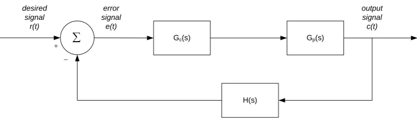
3.2.1 Analogue Controller
In order to understand computer controlled systems, it is first important to briefly
review the analogue controller. The analogue control system is generally comprised of a
summing junction, a controller Gc
( )
s , plant Gp( )
s , and feedback transmittance H( )
s . The analogue controller is generally modelled in the time domain with transferfunctions using the S-Domain. A general form of an analogue control system is shown
in
( )
tFigure 3-1.
Gc(s) Gp(s)
H(s)
desired error output
signal r(t)
signal c(t) signal
e(t) ∑
[image:34.595.117.537.331.453.2]− +
Figure 3-1 Analogue Control System (based on (ELE3105 2007, mod. 1, fig. 1.1) )
Dorf (1992, sec. 1.1, p. 2) notes that feedback systems (closed-loop systems)
provide a measure of the output signal back with the desired signal in order to control
the system; thereby enabling the control system to drive the controller to eliminate error
in the desired output signal. The feedback signal is often amplified during measurement
- H
( )
s .From the control loop shown in Figure 3-1, the University of Southern
Queensland’s Computer Controlled Systems’ Study Guide (2007, mod. 1) suggests that
the basic sequence of events for any analogue controlled system can then be described
as follows:
1. Generate the desired output signal r
( )
t at time t3. Calculate the signal error e
( ) ( ) ( )
t =r t −ct4. Apply the control algorithm to generate control signal m
( )
t5. Output the control signal to plant input
6. Repeat step 1
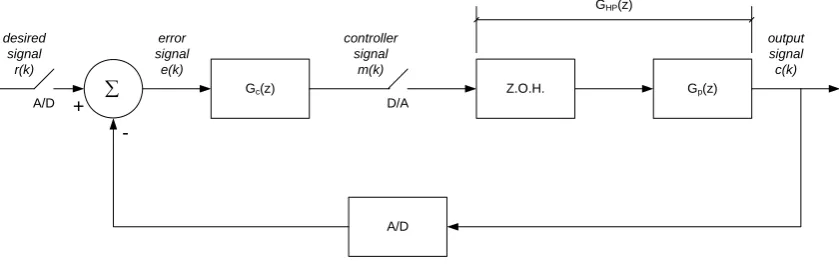
3.2.2 Computer Controller
The computer controller is similar to the analogue controller, however, as the
signals are now digitised, a number of other devices must be considered including
digital-to-analogue converters, analogue-to-digital converters and digital samplers.
Also, as the signals in a computer controlled system are discretised, the computer
controlled system is generally modelled in the discrete time domain with transfer
functions using the Z-Domain. A general form of a computer controlled system is
shown in
[image:35.595.117.537.368.501.2]( )
kFigure 3-2.
Z.O.H. Gp(z)
A/D desired
signal r(k)
output signal
c(k) error
signal e(k) ∑ A/D
Gc(z)
controller signal
m(k) D/A
GHP(z)
+
-Figure 3-2 Computer Controlled System (based on (ELE3l05 2007, mod. 5, fig. 5.1) )
From the digital control loop shown in Figure 3-2, the basic sequence of events
for any computer controlled system can then be described in a similar manner to
analogue systems in the preceding section (refer Section 3.2.1):
1. Generate the desired output r
( )
k for sample k2. Measure the actual output c
( )
k3. Calculate the error e
( ) ( ) ( )
k =r k −ck6. Repeat step 1
3.2.3 Controllers
Now that the control system has been explained, the controller itself can be
discussed. Generically, Leis (2003, mod. 4) suggests that an ideal Controller has three
key characteristics:
a) Fast response,
b) Minimal overshoot, and
c) No steady-state error.
Leis (2003, mod. 4) further suggests that these characteristics can be found by the
combination of the three base Controllers:
a) Proportional Controller – control ∝ error:
i. Increase response speed;
ii. Decrease steady-state error; and
iii. Decrease system damping.
b) Integral Controller – control ∝ accumulated error:
i. Accumulates while there is an error;
ii. Forces steady-state to zero; and
iii. Decreases stability.
c) Derivative Controller – control ∝ rate-of-change-of-error:
i. Brakes the response; and
ii. Makes the response more sluggish.
The three basic controller types – proportional, derivative and integral – can be
practically combined to forma PID Controller. Figure 3-3 shows how a PID Controller
D/A A/D desired signal r(t) controller signal m(t) output signal c(t) error signal e(t) Control Computer
∑ ∑ GHP( )z
( )t e Kp ( ) dt t de Kd
( )tdt e Ki∫
[image:37.595.115.536.56.259.2]PID Controller -+ + + +
Figure 3-3 Digital Control Loop (based on (Leis 2003, mod. 1; mod.4) )
Taking the standard digital control loop, the controller’s signal can then be
mathematically modelled as:
( )
( )
( )
( )
dt t de K dt t e K t e K tm = p + i
∫
+ dEQN 3–1
Where the constants:
time sample is time derivative is constant gain is and , T T K T KT K d d d = EQN 3–4
It can be shown that this function can be transformed to:
( )
(
(
12)
2)
( )
1 1 0 1 − − − − + + = z z E z q z q q zM EQN 3–5
Which can then be represented as a difference equation of:
1 2 2 1 1
0 + − + − + −
= n n n n
n q e qe q e m
m
EQN 3–6
Where the constants:
⎟ ⎠ ⎞ ⎜ ⎝ ⎛ + = T T K q d 1 0 EQN 3–7 ⎟⎟ ⎠ ⎞ ⎜⎜ ⎝ ⎛ − + − = i d T T T T K
q1 1 2
EQN 3–8
T KT
q = d
2
EQN 3–9
Ultimately it is these three constants — — that will be modelled as
Genes within the Genetic Algorithm optimisation presented within this paper using
Argo.
2 1 0,q andq q
3.3
Tuning
In order to achieve the desired performance of the controller the three PID
parameters must be tuned. University of Southern Queensland’s Computer Controlled
Systems Study Guide (2007, mod. 4.2) suggests that tuning can be performed using a
number of methods including:
a) Trial and error,
c) Heuristics (e.g. Ziegler-Nichols),
d) Analytical analysis (e.g. Steepest decent optimisation), or
e) Natural algorithms (e.g. Genetic Algorithm).
This project is fundamentally concerned with providing a Genetic Algorithm from
which to optimise the three PID parameters for a given control system.
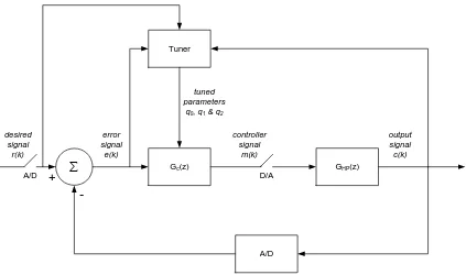
The University of Southern Queensland’s Computer Controlled Systems Study
Guide (2007, mod. 4) also explains that tuning can be either fixed or adaptive. Fixed
tuning selects the controller parameters upon start of the control system, and they
remain as-set whilst the control system is in operation. Adaptive tuning seeks to change
the parameters during operation of the control system in order to provide optimal
control performance by addressing any changes to the control system during operation
(including environmental changes impacting the system).
GHP(z)
A/D
desired signal
r(k)
output signal
c(k) error
signal e(k)
∑
A/D
Gc(z)
controller signal
m(k)
D/A
+
-Tuner
tuned parameters
[image:39.595.115.538.361.611.2]q0, q1 & q2
Figure 3-4 Adaptive Digital Control System
This project will provide a Genetic Algorithm for optimisation of a PID Controller
using fixed tuning only. However, the project will endeavour to explain how it could be
3.4
Summary
In summary, this chapter presented an overview of control systems, providing
models for both analogue and computer control systems. The chapter then discussed the
ideal characteristics for any controller, and provided a mathematical model for a
controller that could achieve these requirements – the PID Controller. Finally, the
chapter briefly discussed methods of how to tune the parameters of the PID Controller,
including:
a) Trial and error,
b) Experimental results,
c) Heuristics (e.g. Ziegler-Nichols),
d) Analytical analysis (e.g. Steepest decent optimisation), or
e) Natural algorithms (e.g. Genetic Algorithm).
This project will use a Genetic Algorithm in order to provide a fixed tuning
Chapter 4
Genetic Algorithms
4.1
Introduction
Before the MATLAB® program Argo can be explained and its interface with a
PID Controller demonstrated, a sound understanding of Biological Genetic Algorithms
must first be gained. To achieve this goal, this Chapter will present the general
principles of Biological Genetic Algorithms including the fundamental concept of
Natural Selection. Once the concept of Natural Selection has been presented, this
Chapter will then explain the basic process that any Genetic Algorithm would follow if
applied to a real-world problem.
In order to understand the capabilities and limitations of applying a Genetic
Algorithm to an engineering optimisation problem, the Chapter concludes with a brief
discussion on the main advantages and disadvantages associated with Genetic
Algorithms.
4.2
Biological Genetic Optimisation
Genetic Algorithms are simply a series of steps for solving a problem whereby the
problem-solving method uses genetics as the basis of its model (Chambers 2005,
preface). Genetics is the branch of biology that studies how parent organisms transfer
their cellular characteristics to children. Genetic Algorithms attempt to model the
concept of Natural Selection within genetics, whereby Chambers (2005, preface)
“… organisms most suited for their environment tend to live long
enough to reproduce, whereas less-suited organisms often die before
producing young or produce fewer and/or weaker young”.
Implicit in the concept of Natural Selection is the idea that the stronger organisms
live long enough to reproduce often and pass their genetic traits on to their offspring,
whereas because the weaker organisms do not produce as many offspring their genetic
traits are not as prolific within the population.
At the cellular level a gene is the basic unit of heredity (Haupt & Haupt, 2004,
sec. 1.4). The gene contains information that describes a specific trait of an organism.
Multiple genes are combined to form a chromosome – the sequence of genes within the
chromosome is often referred to as the organism’s genetic code (Haupt & Haupt 2004,
sec. 1.4). One common implementation for a Genetic Algorithm is to code
chromosomes and genes as a string of bits. Individual bits in the encoded string are
analogous to the genetic concept of an allele (Whitley n.d., p. 16).
For a Genetic Algorithm to model the real world, the first important step is that of
selection. Selection is the process where organisms are chosen to mate and produce
offspring (Haupt & Haupt 2005, sec. 2.2.5). Natural Selection often occurs in nature by
mating two parents to produce one offspring. Although Genetic Algorithms are not
necessarily limited to a set number of parents, it is common to select only two parents
for mating. Argo requires the selection of two parents for mating which in turn produces
two offspring.
Once two offspring are selected mating occurs. Mating is the process that mimics
sexual recombination of cells. Genetic Algorithms perform mating by a process of
crossing chromosomes. Crossing is a process whereby two parent cells divide and then
arrange themselves such that they recombine to form offspring that have part of their
chromosome provided by both parents. Crossing mimics the genetic process of meiosis
that results in cell division (Haupt & Haupt 2004, sec. 1.4) – reproductive cells divide at
a random point along the chromosome known as the kinetochore (Haupt & Haupt 2004,
sec. 1.4).
A rare but important part of mating is mutation. Chambers (1995, p. 48) explains
that mutation “is the process of randomly disturbing genetic information”. Mutation
chromosome. Similar to nature, Genetic Algorithms seldomly apply the process of
mutation. Natural Selection leads to the maintenance of a strong genetic population
through heredity of strong genes. Mutation counters this, and hence is used to
reintroduce alleles/genes that may have been lost in the population after selection and
crossing but which actually make the chromosome stronger in terms of its environment.
Genetic Algorithms apply mutation in order to avoid prematurely converging to a
sub-optimum genetic solution.
4.3
Genetic Algorithms
Obviously nature applies the processes of selection, mating, crossing, mutation
and reproduction continuously whilst ever the species continues to survive. However,
Genetic Algorithms are an optimisation and search technique based on the principles of
genetics and natural selection in order to maximise genetic fitness (Haupt & Haupt
2004, sec. 1.5). Often Genetic Algorithms encode the parameters of a real-world
problem and then attempt to maximise an associated fitness function (Whitley n.d., p.
1). Thus, whereas nature applies the process of natural selection continuously, Genetic
Algorithms apply the process iteratively until a set of encoded parameters is found that
maximises the modelling function. Hence Genetic Algorithms are often used as a
function optimising technique.
The key difference between Genetic Algorithms and analytical optimisation is that
in effect Genetic Algorithms are a population-based model that searches the fitness
space to find the optimum parameters (Whitley n.d., p. 1). Whereas analytical
optimisation attempts to mathematically model the process and optimise using either
calculus or numerical techniques.
4.4
Advantages and Disadvantages
As already eluded to, Genetic Algorithms have numerous inherent advantages
over classical numerical optimisation techniques. Haupt & Haupt (2005, sec. 1.5) attest
that some of the advantages of Genetic Algorithms are that they:
a) Can handle discrete and continuous variables;
c) Are suited to parallel computing (still the current means from which
personal computers are attempting to gain significant increases in
processing power);
d) Can provide a list of optimal variables;
e) Can handle complex cost surfaces (local minima/maxima do not falt the
method); and
f) Can handle large numbers of variables.
However, despite the many advantages over classical analytical optimisation
techniques, the Genetic Algorithms own process of searching a large solution space
results in a significant disadvantage. That disadvantage being a high computational cost
associated with processing and searching a large solution space. Such a computational
cost is normally manifested by a slow computational process and a high demand for
memory. Hence, classical analytical optimisation techniques still remain the best for
complex analytical functions with few variables.
4.5
Genetic Algorithm Process
4.5.1 Problem Definition and Encoding
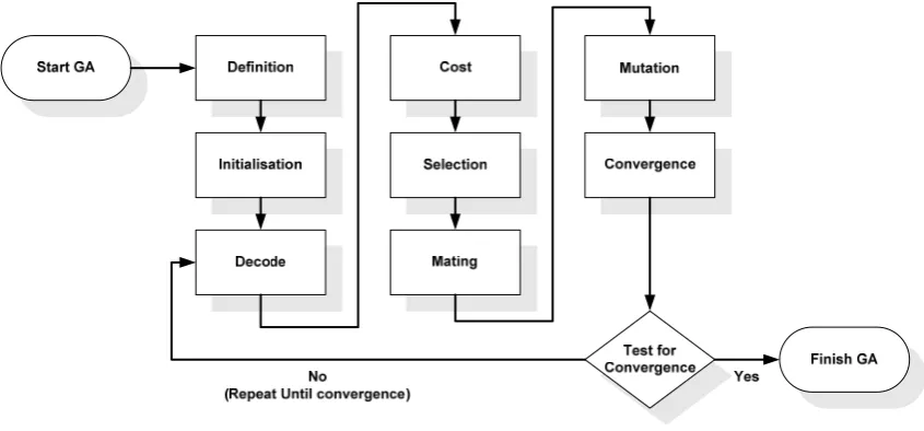
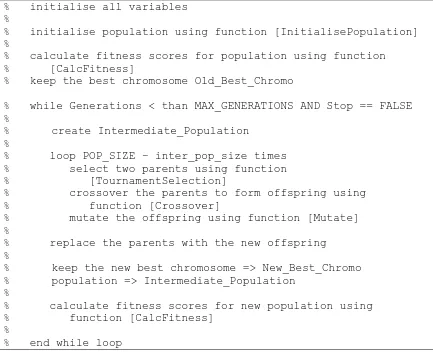
The generic Genetic Algorithm process is shown in Figure 4-1 Biological Genetic
Algorithm Process Flow. The process commences with the definition of the problem
and the encoding of chromosomes from which to apply the Genetic Algorithm process
digitally.
This step is also important as the convergence criteria must be defined. The
convergence criterion defines the situations under which the Generic Algorithm will be
Figure 4-1 Biological Genetic Algorithm Process Flow
4.5.2 Initialisation
Once coding of chromosomes is defined, the starting population of chromosomes
within the search space can be initialised. The process of initialisation can be tailored
dependent upon the problem and how the system operates in practise. For example,
initialisation could be achieved by setting all chromosomes to be the same sequence
with the chromosome value being arbitrarily chosen, selected at random or specifically
nominated. Regardless, this method is not normally recommended as the Genetic
Algorithms strength lies in its ability to provide and search a diverse solution space, and
this method slows the diversification of the population – and hence slows the
optimisation process in general. However, the speed of the optimisation problem could
be increased if the arbitrary value representing the chromosome was known to be near
the optimal value.
Nevertheless, if the optimal value for a chromosome is unknown, the best
initialisation method of the population is to randomly assign values to all chromosomes
within appropriate limits for the system variables that the chromosomes are modelling.
4.5.3 Decoding
4.5.4 Cost
Once each chromosome has been decoded, the chromosome’s cost can then be
calculated. The cost function is normally a mathematical function, but, it could be
programmed to be derived from an experimental result or even an outcome from a game
(Haupt and Haupt, 2004, sec 2.2.1). Referring to the generic optimisation model
presented in Chapter 2 (refer Section 2.2), the cost is the system’s output derived from a
set of inputs. Further, the cost can also be considered to be the difference between the
actual output value for the given set of inputs and the optimal output (Haupt and Haupt,
2004, sec 2.2.1).
As previously discussed in Chapter 1 (refer Section 1.4.1), Whitley (n.d.)
prescribes that there is a difference between the evaluation and fitness functions within
the Genetic Algorithm. The evaluation function determines the cost independent of
evaluation of other chromosome’s cost. Whereas the fitness function determines the
cost of the chromosome relative to all other chromosome’s within the population.
Practically this could take the form of a simple sorting algorithm.
4.5.5 Selection
Once each chromosome’s cost has been calculated, the Genetic Algorithm can use
this data to determine which chromosomes should be selected to mate. The selection
function is generally the aspect that contains the most differences between Genetic
Algorithms and arguably has the greatest impact upon the Genetic Algorithm’s eventual
success.
A number of selection methods have been proposed including:
a) Ranked pairing,
b) Random pairing,
c) Weighted random pairing, and
d) Tournament Selection.
Ranked pairing is a simple selection method whereby two adjacent chromosomes
are selected from a rank sorted list, whereby ranking is based on cost. Extensions to this
1.14.1.4). Fit-Fit (pairing with next fittest chromosome) is highly conservative
compared to Fit-Weak (pairing with next weakest chromosome) which is highly
disruptive of the genetic information. Obviously ranked pairing does not follow nature’s
model, however, it is simple to program (Haupt and Haupt, 2004, sec. 2.2.5). This
method also has the computational penalty of requiring a sort of each population.
Random pairing is also a simple selection method whereby two chromosomes are
selected at random from the population, regardless of ranking. This method has some
similarities with nature, and, has the added advantage of not requiring the computational
cost of sorting each population.
Weighted Random selection, also known as Roulette Wheel selection, is one of
the most common selection methods used in practical Genetic Algorithms. Roulette
Wheel selection is based on its namesake whereby each slot in the wheel is weighted in
proportion to its fitness. Hence, selection is more likely for fitter chromosomes. A
random number is used to determine which chromosome on the Roulette Wheel is
selected. Weighted Random selection can be refined by using either the ranking or the
cost to calculate the probability of selection (Haupt and Haupt, 2004, sec. 2.2.5). This
method has similarities with nature, as it attempts to provide a model that mimics the
concept of Natural Selection. However, this method is computationally expensive. Also,
Chambers (1995, Sec 1.14.1.1) notes that this method is “only a moderately strong
selection technique, since fit individuals are not guaranteed to be selected for, but have a
somewhat greater chance”. Chambers (1995, Sec 1.14.1.1) also warns for practical
application that it is essential not to sort the population, as this will dramatically bias the
selection.
Haupt and Haupt (2004, sec. 2.2.5) suggests that Tournament Selection is perhaps
the method that most closely mimics nature. This method identifies a pool of candidate
chromosomes at random and then selects the fittest candidate as the first successful
parent. This method has the added advantage of not requiring the computational cost of
sorting each population.
4.5.6 Mating
that point (Haupt and Haupt, 2004, Sec 2.2.6). Multiple crossover points can be used,
however, the greater the number of crossover points used the greater the disruption of
the genetic information in the population. Normally the crossover point itself is chosen
at random from the genetic code (Haupt and Haupt, 2004, Sec 2.2.6).
4.5.7 Mutation
Mutation is a change in a gene’s characteristics. The change occurs randomly in
order to re-introduce/introduce genetic traits not found in the population. This process is
key to a Genetic Algorithm’s ability to eventually converge on the global optimal
solution – mutation helps prematurely converging on a local minima/maxima.
However, mutation by concept is disruptive. Therefore, the mutation rate for most
Genetic Algorithms is very low, often in the order of 1% or lower. Also, it is normal
practice for most Genetic Algorithms not to allow mutation on the current fittest
chromosome.
Practically, mutation on a binary encoded Genetic Algorithm is simply a change
in an allele’s value from a ‘1’ to a ‘0’ or vi