The GDS model - a rapid computational technique for the calculation of aircraft spray drift buffer distances

The GDS model – a Rapid Computational Technique for

the Calculation of Aircraft Spray Drift Buffer Distances

I. P. Craig

The University of Southern Queensland, Toowoomba, Australia

Please note this is the original draft form only – please refer to officially published version in - Computers and Electronics in Agriculture 43 (2004) 235-250

Abstract

A model for predicting the required spray drift buffer distance for a specified off target deposition level is described. The GDS model is based upon Gaussian diffusion and

sedimentation of particles originating from an elevated instantaneous line source. Aircraft-induced near wake effects are ignored. Agreement between aircraft wake models FSCBG, AgDRIFT and the GDS model is reasonable for downwind distances greater than 50m. The model has the advantage over Lagrangian models in that it is faster computationally and can readily provide real time prediction in the cockpit over large distances (3 km). A sensitivity analysis has been performed on the model to elucidate the effects of the primary parameters on spray drift. The model has proved useful in the determination of spray drift buffer distances for regulatory purposes and in the development of appropriate spray drift management systems for aerial spraying. Further research work is required to refine the model to better account for air stability effects, collector type, evaporation and crop canopy.

Keywords: Spray drift, Gaussian Diffusion, Sedimentation, Buffer Distance

1 Introduction

The dispersal of material released from aircraft, in particular low flying aircraft applying pesticides, is a subject of interest because chemical residues need to be effectively managed for human health, environmental and trade reasons. As with most problems involving dispersal of a continuous slug of material near to the source, rather than isolated puffs at distance, the Gaussian distribution provides the most useful first approximation.

Gaussian type equations which simulate the atmospheric diffusion (or dispersion) of particulate materials are described in texts including Turner (1970), Csanady (1973), Hanna et al (1982), Pasquill and Smith (1983) and Panofsky and Dutton (1984). Elevated line source versions of these equations to simulate aerial release were developed and validated by Cramer et al (1972) and Bache and Sayer (1975). The Bache and Sayer or “Cranfield” model was validated experimentally at Cranfield Aerodrome UK in 1973. A simpler time independent expression was developed by Lawson (1978) and Spillman (1982) which forms the basis of the model described here.

Other models use Lagrangian methods to track a large number of particles to simulate complex source conditions incorporating aircraft wake, wing tip and propeller vortices (Reed 1953, Trayford and Welch, 1977). During the 1970s the US Army and the US Forest Service developed programs to simulate aerial spraying, which were validated experimentally at the Dugway Proving Ground, Utah. By the 1980s, two programs became available :- AGDISP (Bilanin et al 1989) and FSCBG (Grim and Barry 1975, Dumbauld et al 1976). FSCBG starts with AGDISP (Lagrangian) and “hands over” to a Gaussian algorithm for far downwind distances. AGDISP was later developed into AgDRIFT for pesticide registration purposes in the United States (Teske et al., 1997). AgDRIFT allowed for the position of each individual nozzle on the aircraft and was validated experimentally in trials funded by the Spray Drift Task Force (SDTF) which took place in 1992/3 at Plainview, Texas.

Gaussian models, however, can provide an inaccurate prediction of near field deposition (< 50m downwind of spray release). Instead of a single large peak, aircraft spray booms close to the ground generally produce two or three smaller peaks, starting further upwind compared to the Gaussian model. These peaks may be due to turbulence caused by wingtip vortices and propeller wake. To improve accuracy in the near field a Lagrangian solution is required. However, accuracy in the near field does not necessarily seem to be a prerequisite for accuracy in the mid and far fields. Good agreement between the outputs of Gaussian and the FSCBG model were obtained by Dorr (1996) who concluded that the Gaussian approach was adequate for downwind distances greater than 50m.

Lagrangian models which compute the trajectory of plume centres within a flow field are now the accepted approach for air pollution/odour modelling. This method is necessary where the pollutant is in the form of a gas molecule or very small particle with a long airborne

residence time requiring spatial and temporal meteorological data to be entered into the model. With aircraft application, however, most of the droplets are large enough to be deposited within the mid field within a few minutes of release, during which time constant

meteorological conditions can be assumed. This offers a considerable saving in terms of computational requirements. Software updated with new windspeed and direction information only every minute or so might be appropriate.

2 Method

2.1 Basis of model

The GDS model assumes that the plume containing diffusing and settling particles

originates from an elevated, instantaneous, infinitely long line source. The model can therefore only be safely applied if the length of the sprayed area (dimension perpendicular to mean wind direction) is as least as large as the downwind distance of prediction. The model assumes a uniform atmosphere and 100% capture of droplets reaching ground level ie. no reflection.

Turbulence intensity (defined as i = u*/u where u* is the RMS of vertical air motion) essentially controls the rate at which the drifting droplet cloud expands and dissipates and this affects the shape deposit pattern (Fig. 1)

Figure 1

The standard deviation of vertical spread of the cloud is equated to ix, where x is the downwind distance. The default value of i is 0.1 which is equivalent to Pasquill “B” class stability at 500m downwind of the source. For an instantaneous line source with strength q, the deposit d, may be expressed as

   

 − −

= _{½ 2 2} 2

) ( 2

) (

exp )

2

( ix

u x v h ix

qh

d s

π (1)

where h is the release height, vs is the sedimentation velocity of the droplet and u is the mean windspeed. The result is weighted according to a particular droplet diameter distribution and summed for multiple line sources according to the number of crosswind spray runs.

2.2 Types of spraying

Spray application of pesticides, still necessary for the production of many crops, may be categorised into three major types as follows :

2.2.1 Ultra Low Volume (ULV)

surfaces and therefore high efficacy. This technology is particularly suited to the control of airborne locusts, tsetse fly (Andrews et al 1983) and in forestry (Crabbe et al 1994) where there are vast areas of tall canopy to be penetrated. ULV application has also been successfully utilised in the production of cotton in Africa, Asia and Australia. The technique has proved highly efficacious and cost effective, but can have higher drift compared to other methods.

2.2.2 Low Volume (LV)

Low Volume (LV) involves water based application at bulk rates of 10-30 litres per

hectare using standard hydraulic nozzles. Droplet VMD is usually between 100µm and 250µm. Low Volume or LV spraying is the most common method of applying agricultural pesticides in Australia (Woods et al 2000). The method uses a water based carrier to dilute the pesticide product which may be an Emulsifiable Concentrate (EC) or a Suspension Concentrate (SC). Nozzles are usually hydraulic with flat fan or deflector types being the most common. Spray drift levels associated with LV application are generally at an intermediate level between those associated with ULV and LDP application.

2.2.3 Large Droplet Placement (LDP)

Large Droplet Placement (LDP) spraying is defined by Craig et al (1998a) as water based spraying with a droplet VMD greater than 250µm. Bulk application rates are usually 30 to 100 litres per hectare to ensure adequate plant coverage (usually defined as numbers of droplets per square cm on crop surfaces). Large droplets have high sedimentation velocities and are not greatly influenced by vertical air movement and turbulence. LDP methods should therefore be used to reduce spray drift when spraying has to be undertaken close to susceptible areas.

2.3 Droplet VMD data

Equation (1) is solved for 40 droplet diameters from 5 to 1800µm, each associated with a particular sedimentation velocity. The result is weighted according to its frequency in a particular droplet diameter distribution. Distributions obtained using laser droplet sizing or other methods can be entered into the model. Actual data for a specific nozzle, formulation and airspeed may be entered into the GDS model, in addition to BCPC or ASAE International Reference Spectra (Hewitt and Valcore, 1998).

frequency distributions are commonly normal or bell shaped if plotted against log droplet diameter. Where is X is log10 droplet diameter, σL is the standard deviation of log10 droplet diameters and µ is log10 droplet VMD, or dv0.5, the frequency distribution based on volume is generated as

   

 − − =

L L

X k

X f

σ µ σ

π 2

) (

exp )

2 ( ) (

2

½

(2)

where and k≈ 6.4 to make the sum equal 100%. Log normal distributions with droplet VMD = 70, 100, 140, 180 and 250µm are plotted cumulatively in Fig. 2. σL is kept constant, making the slopes of the curves equal, a common trend in laser derived data for aircraft nozzles (Craig 1991, Kirk 1997, Woods et al 2000). Relative Span (RS), or [dv 0.9-dv 0.1]/dv0.5, the more

conventional measure of distribution width, varies from approximately 1.5 to 1.3 through the 70 to 250µm range. For the purposes of this paper, the 70µm, 180µm and 250µm droplet VMD curves with σL equal to 0.2, have been determined as representative of ULV, LV and LDP aerial application respectively (Woods et al 2001).

Figure 2

2.4 Overlap Routine

Using an overlapping (summing) procedure, the GDS model spreadsheet is capable of predicting a 2D profile of drift deposition downwind from a sprayed area. If the cell resolution is 5m or less, deposition within the sprayed area can be depicted (Fig.3). The model is

normally set up with a cell resolution of 20m, which enables it to calculate deposition over a combined Field Source Length (FSL) ie. length of sprayed area parallel to mean wind direction plus downwind distance of approximately 5km.

2.5 Effect of Stability

The value i, which controls the rate of expansion of the cloud, can be adjusted to simulate dispersion in unstable, neutral and stable conditions (Pasquill and Smith, 1983). Crabbe et al (1994), Bird et al (1996), Miller et al (1999) and Thistle (2000) confirm that the effect of stability is to significantly increase spray drift deposition values recorded close to ground. Further work is required to adapt the GDS model for super stable or temperature inversion conditions. Algorithms do exist for Gaussian air pollution models (without sedimentation) to account for inversion capping which may be of assistance in this task.

2.6 Effect of Collection Surface

What the GDS model and most models calculate, is not deposition of particles or droplets upon a solid surface, but rather the flux of these particles through an imaginary plane at height zero. This is as though the droplets together with the air that they are travelling with were able to pass through the ground surface as if it was not there. In reality of course, the ground surface does exist and acts to deflect the air and droplets. Large droplets have sufficient momentum to depart from the deflected airsteams and deposit on the ground. Small droplets on the other hand move with the air and are not readily deposited, unless they encounter a target with a very small dimension such as a blade of grass or leaf hair. The air deflection around small objects is minimal allowing deposition of small droplets to occur (May and Clifford, 1967).

In this case, deposition is not strictly at height zero and the air is able to keep flowing to a point below the deposition of the droplet. However, if the canopy height is small compared to the release height of the spray, these deposition heights can be regarded as very small and can be ignored. A rough surface with high catch efficiency, such as a grassed field, can therefore be assumed to approximate flux through an imaginary plane. Some of the difficulties in properly assessing long distance deposition of aerosol (<30µm) droplets on smooth surfaces, such as alpha-cellulose sheets, are therefore highlighted (Craig et al 2000).

2.7 Effect of Droplet Evaporation

evaporate completely. This acts to reduce the source strength of the cloud as it progresses downwind. The net effect may be to slightly reduce ground deposition rather than increase it.

The recent data provided by Woods et al (2001) compares the drift profiles generated by oil versus water based aerial spraying methods. There was good agreement between the data and the outputs from both AgDRIFT (evaporating) and GDS model (non evaporating) models. The oil and water based data were similar suggesting that the net effect of evaporation on deposition is small. It is reasonable to assume that in hot conditions evaporating droplets diminish to their involatile diameters relatively quickly after release. It may therefore possible to make small adjustments to the droplet VMD entered into GDS model to account for

evaporation. Further experimental work on evaporation (Riley et al 1995) is required to evaluate the magnitude of this correction appropriate for different types of spray formulation and to develop suitable algorithms.

2.8 Effect of Crop Canopy

The effect of a crop canopy is important for ground boom spraying where nozzles are close to crop surfaces. The effect can be considered as an initial source strength reduction due to filtration of droplets by the crop. The effect is probably less than a few percent and can be ignored with aerial application where the spray nozzles are usually well above the crop canopy. Drifting droplets, once above the canopy, are “unlikely to ever again to experience the vicinity of the canopy” (Holterman et al . 1997).

A simple function to approximate initial removal of the spray by the crop canopy has been adopted for the GDS model. The spray source is assumed to consist of a hydraulic nozzle emitting droplets horizontally with a mean direction of travel parallel to the mean wind direction. The spray cloud is assumed to have a Gaussian vertical concentration profile, depicted with a spread of ± 3σ (Fig. 4). Since the downwind distance x is relatively small (≈10σ), sedimentation of the cloud is ignored.

This approximation to account for crop canopy proximity must be applied with caution as experimental validation of the method is required. Crop canopy effects are in reality much more complicated and the GDS model requires canopy algorithm based upon experiments with individual canopy types and studies which have properly related filtration to canopy

dimension, porosity and airflow within the canopy (Holterman et al 1997 and Raupach et al. 2001).

Figure 4

3 Results and Discussion

3.1 Model Validation

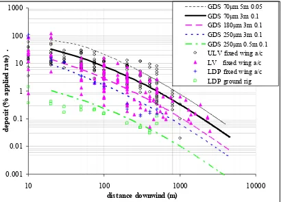
GDS model predictions of downwind deposition (expressed as % applied rate) with distance are presented in (Fig 5). The uppermost curve (high drift case) has spray release height set to 5m, and turbulence intensity set to 0.05. The next three curves progressing downwards correspond to droplet VMD set to 70µm (ULV), 180µm (LV) and 250µm (LDP) and default parameters (eg. height = 3m, i = 0.1) as described in Table 1. For purposes of comparison, a fifth (lowermost) curve was added corresponding to ground rig application with a 0.5m release height and a droplet VMD of 250µm (LDP).

The curves are overlaid with field trial data points obtained using gas chromatography analysis of paper covered horizontally oriented flat plates (Woods et al, 2001). Other data points for a helicopter 250µm (LDP) application are not shown here, but plotted between the two lower curves, agreeing perfectly with the GDS model when the spray release height was set to 1m.

Taking an average across the fixed wing aircraft ULV and LV data, deposition fell to 1% of the field applied rate at approximately 500m downwind of a 500m wide sprayed area. For aerial LDP application, deposition fell to 1% of the field applied rate at approximately 150m downwind. This percentage compares with 0.5% at 150m downwind, quoted for the US Spray Drift Task Force (SDTF) data (Bird et al 1996).

spraying (the applications were not instantaneous) may also have caused some variability. Despite this, however, the data taken overall supports the GDS model predictions.

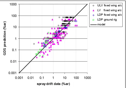
Fig. 6 is an experimental data versus model prediction plot of the same deposition data (% applied rate) represented in Fig. 5. Logarithmic transformation of the data has been performed to avoid the least squares regression method being heavily weighted towards samples near the spray source, where deposit values are several orders of magnitude greater than those further downwind. With all of the data pooled together (Fig. 6), a clear correlation is apparent between the GDS model and data, with the 1:1 line (slope = 1.0, representing 100% agreement with the model) being centrally placed amongst the points.

Figure 5

Figure 6

Agreement of the data with GDS model predictions is best summarised by the statement “approximately 90% of measurements were within a factor of five of the model prediction”. A similar level of agreement was demonstrated for the SDTF data when compared to AgDRIFT model predictions (Bird et al 1996, Teske et al 2000). Richardson et al (1995) also quotes “factor of five” agreement for single flight line drift data obtained in New Zealand, when compared with FSCBG model version 4.0 and 4.3 predictions. The authors noted that FSCBG based Lagrangian predictions of peak deposition value distance were not always reliable, and so only the Gaussian (35m to 300m downwind) portion of FSCBG was used in this analysis. Some Lagrangian over prediction close to the spray source (using AgDRIFT version 1.05) was also evident with the present data set (Woods et al 2001).

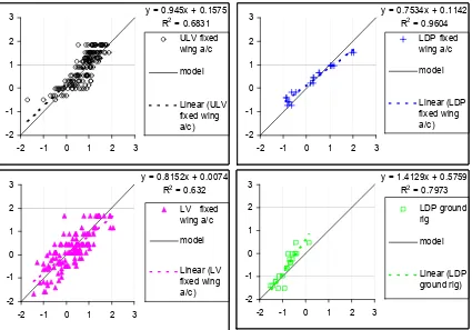
Figure 7

Fig. 7 represents the same data split into the four different treatments – aerial ULV, aerial LV, aerial LDP and ground rig LDP. Looking at the aerial ULV data alone, reasonable

data, model agreement is still reasonable (slope = 0.815, R2 = 0.63). With the aerial LDP data, the GDS model slightly under predicts deposition close to the source (slope = 0.75, R2 = 0.96) but with the ground rig LDP data the GDS model over predicts deposition close to the source (slope 1.41, R2 = 0.8). This may be due removal by the crop canopy of larger droplets

depositing near source- an effect not properly accounted for with the existing GDS model.

3.2 Determination of Buffer Distance

The GDS model can be used to calculate buffer distances required for off target downwind deposition levels to fall below a specified threshold level. This level can either be expressed as a percentage of the active ingredient rate applied (independent of chemical type) or as a

Predicted Environmental Concentration (PEC). Threshold levels, usually quoted in ppm, vary widely according to the chemical and the sensitive target concerned.

For the purposes of this paper, an off target deposition level of 0.1% of the field applied rate was chosen as the threshold level upon which generic buffer distances may be determined. This is because this level roughly corresponds to the No Effect Level (NOEL) for a number of herbicides applied to sensitive downwind crops and also the maximum residue levels (MRL) permitted for livestock feed for some of the older organochlorine/organophosphate insecticides (Akesson and Yates, 1964). Referring to Fig. 5, generic buffer distances of approximately 2km, 1km, 750m and 200m may be ascertained for aerial ULV, LV, LDP and ground LDP application, based on the constants defined in Table 1.

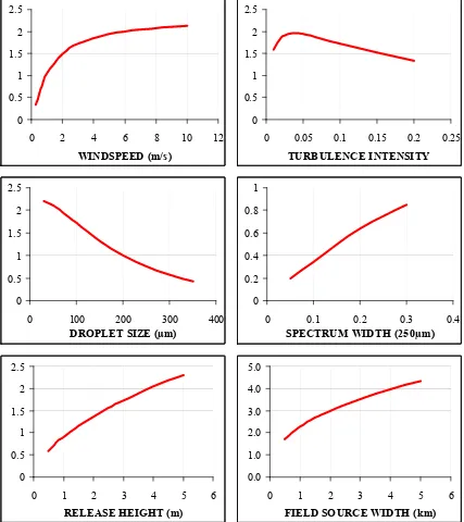
3.3 Sensitivity Analysis

A sensitivity analysis was performed by varying one parameter at time. Default values for the parameters kept constant are given in Table 1. The trends depicted (Fig. 8) are broadly in agreement with the FSCBG and AgDRIFT Lagrangian based models (Woods et al 2001).

Table 1

3.3.1 Windspeed

With 100µm droplets, the effect of windspeed is important, initially, up to about 3 m/s. Above 3m/s however, there is only a marginal increase in the required buffer distance. This has an important implication on the determination of upper windspeed limits in ULV spray drift management programmes. With larger droplet VMD, spray drift values are less overall and the effect of windspeed is more linear. In practice, it is important to have a lower limit (commonly 0.5m/s) which avoids spraying in stable conditions or when the direction of the wind is unpredictable.

3.3.2 Turbulence intensity

Turbulence intensity value i determines the rate at which the spray cloud expands and dissipates. The lower the value of i, the more concentrated the spray cloud remains near ground level and in general, the higher ground deposition levels are, both within the sprayed field and downwind of the field. Under neutral conditions with a breeze over a crop, it is reasonable to assume i = 0.1 although this value can be adjusted to 0.2 for unstable conditions over a rough surface, or to 0.05 for stable conditions over a smooth surface eg. grass. With distance to 0.1% applied rate used as the drift index, maximum distances for a 100µm spray occurred when i

was equal to about 0.03. Low turbulence intensity values occur when cooling of the ground at dusk causes a strong positive temperature gradient. The turbulence intensity in this layer can be extremely low, resulting in arrested diffusion of aerosol (< 30µm) droplets close to ground level and high residue levels several km from the spray source.

3.3.3 Volume Median Diameter

3.3.4 Spectrum width

The effect on spray drift of varying σL was investigated with a 250µm droplet VMD spray only, because when droplet VMD is less than 200µm, the effect of σL becomes small. For a 250µm VMD spray, σL is typically 0.2 (RS ≈ 1.3) for water based hydraulic nozzle and rotary cage sprays where airstream breakup is the main mode of atomisation. However, σL can exceed 0.3 (RS ≈ 2) depending on the nozzle type, flowrate, formulation and other parameters (Woods et al 2000). If σL could be reduced to 0.1 (RS ≈ 0.6) for a 250µm VMD spray, with specialised nozzles as described by Craig et al (1998b), required aircraft spraying buffer distances would be significantly reduced.

3.3.5 Release height

The predicted relationship between spray release height and distance required for 0.1% applied rate forms a gentle curve. As a general rule, buffer distance may be described as varying approximately as the square root of spray release height for 100µm droplets, for the range of spray release heights normally encountered in agricultural spraying.

3.3.6 Field source length

4 Conclusion

A simple Gaussian Diffusion Sedimentation (GDS) model has been presented to predict off-target spray drift deposition associated with aircraft spraying activities. The model incorporates the basic parameters of windspeed, air stability, droplet VMD, spectrum width, release height and field source length. The main advantage of using the Gaussian Diffusion Sedimentation (GDS) model is computational speed, as it constitutes a statistical rather than a Lagrangian (particle tracking) approach. The latter is required for modelling in the near field (under the aircraft and out to ~50m downwind). The GDS model is more suited to prediction in the 50m to 3km downwind range.

Correlation has been presented between GDS model output and some spray drift deposition data collected on paper covered plates placed downwind of sprayed fields. Some data points were up to five times higher than the GDS model prediction due to uncertainties in the measurement of air stability during the trials. Others were up to five times lower than the GDS model prediction due to variability in wind direction during the trials ie. the collectors “missed” the drifting spray plume. The variability in the data (± 5 x mean) is similar to that in other similar studies.

5 Symbols used

d deposit, g/m2 h release height, m

q line source strength, g/m

i turbulence intensity x downwind distance, m

v sedimentation velocity, m/s u mean windspeed, m/s u* RMS vertical air motion, m/s

X log10 droplet diameter

µ log10 droplet VMD

σL standard deviation of log10 droplet diameters k constant approximately equal to 6

6 References

Akesson, N.B. and Yates, W.E 1964 Problems relating to application of agricultural chemicals and resulting drift residues. Ann Rev Entomol 9 285-318

Andrews, M., Flower, L.S., Johnstone, D.R. and Turner, C.R. 1983 Spray droplet assessment and insecticide drift studies during the large scale aerial application of endosulfan to control Glossina morsitans in Botswana. Tropical Pest Management 29(3):239-248 Bache, D.H. and Sayer, W.J.D., 1975 Transport of aerial spray I : A model of aerial

dispersion. Agricultural Meteorology, 15, 257-271.

Bals, E.J. 1970 Rotary Atomisation. Agricultural Aviation 12 85-90

Bilanin, A.J., Teske, M.E., Barry, J.W. and Ekblad, R.B. 1989 AGDISP: The aircraft dispersion model, code development and experimental validation. Trans ASAE 32:327-334

Bird, S.L, Esterly, D.M. and Perry, S.G. 1996 Atmospheric Pollutants and Trace Gases – Off target deposition of pesticides from Agricultural Aerial Spray Applications J. Env. Qual. 25:1095-1104

Crabbe, R.S., M.McCooeye, Mickle, R.E. 1994 The influence of atmospheric stability on wind drift from Ultra-Low-Volume aerial forest spray applications. Journal of Applied Meteorology 33 500-507

Craig I.P., Woods N, and Dorr, G. 1998a A simple guide to predicting aircraft spray drift. Crop Protection 17 (6) 475-482.

Craig I.P., Woods N, and Dorr, G., 1998b Aircraft spraydrift and the requirement for improved atomiser design. ILASS Americas 11th Annual Conference on Liquid Atomisation and Spray Systems, Sacramento, CA, May 1998 65-69

Craig, I.P. 1991 Fluid Driven Rotary Atomiser for Controlled Droplet Application of Herbicides. Ph.D. thesis 1991 - unpublished. Cranfield University, Bedford, UK. Cramer, H.E. 1972 Development of dosage models and concepts. Contract

DAAD09-67-C-0020(R) with the U.S. Army, Final Report No DTC-TR-72-609, Dugway Proving Ground, Utah.

Csanady G.T. 1973 ‘Turbulent Diffusion in the Environment’. D.Reidel Publishing Company, The Netherlands

Dorr, G. 1996 The Aerial Transport of Pesticides : Validation of Gaussian Plume Models. PGDip thesis, Gatton College, University of Queensland.

Dumbauld, R.K., Rafferty, J.E., and Cramer, H.E. 1976 Dispersion - deposition from aerial spray releases. 3rd symposium on Atmosheric Turbulence, Diffusion and Air Quality sponsored by the Am. Met. Soc. Oct 19-22, 1976, Raleigh, North Carolina.

Grim, B.S. and Barry, J.W. 1975. A canopy penetration model for aerially disseminated insecticide spray released above coniferous forests. Report MEDC-2425. USDA Forest Service, Missoula, MT.

Hanna, S.R., Briggs, G.A., and Hosker, R.P. 1982 Handbook on Atmospheric Diffusion. US Dept of Energy.

Hewitt, A.J. and Valcore, D.L 1998 The measurement, prediction and classification of agricultural sprays. Paper No. 981003, ASAE meeting, July 13-16, Orlando.

Holterman, H.J., Zande, J.C., Porskamp, H.A.J., Huijsmans, J.F.M. 1997 Modelling spray drift from boom sprayers. Computers and Electronics in Agriculture 19 1-22

Kirk, I.K. 1997 Application parameters for CP nozzles. ASAE Meeting Paper No AA97-006, Nevada, 1997

Lawson, T.J. 1978 Particle transmission and distribution in relation to the crop. International Aerial Application of Pesticides shortcourse notes, September 1978. Cranfield Institute of Technology, Bedford, UK (available in Cranfield library).

Miller, D.R., Stoughton, T.E., Thorpe, K., Podgewaite, J. Steinke, W.E., Huddleston, E.W. and Ross, J.B. 1999. Air stability effects on spray drift. Paper AA99-003, ASAE meeting, Reno, Nevada, Dec 13, 1999

Panofsky, H.A. and Dutton, J.A. 1984 Atmospheric Turbulence, John Wiley NY

Parkin C.S and Siddiqui, H.A. 1990 Measurement of drop spectra from rotary cage aerial atomisers. Crop Protection 9 35-38

Pasquill, F. and Smith, F.B. 1983 Atmospheric Diffusion, 3rd ed. Halsted Press New York Raupach, M.R, Woods, N., Dorr, G., Leys, J.F. and Cleugh, H.A. 2001. The entrapment of

particles by windbreaks. Atmospheric Environment 35 3373-3383

Reed, W.H. 1953 An analytical study of the effect of airplane wake on the lateral dispersion of aerial sprays. NACA TN 3032. Nat. Adv. Cttee. on Aeronautics, Langley, Va

Riley, C.M., Sears, I.I., Picot, J.C. and Chapman, T.J. 1995 Description and validation of a test system to investigate the evaporation of spray droplets. ASTM Pesticide Formulation and Application Systems

Richardson, B., Ray, J.W., Miller, K.J.,Vanner, A.L. and Davenhill, N.A. 1995. Evaluation of FSCBG – an Aerial Application Simulation Model. Trans ASAE 11(4) 485-494

Spillman J.J. 1982 A Rapid Method of Calculating the Downwind Distribution from Aerial Atomisers. College of Aeronautics Memo No. 8224. Cranfield Institute of Technology, Bedford, UK, and EPPO Bull. 13(3) : 425 - 431

Spillman J.J. 1984 Evaporation from freely falling droplets. Aeronautical Journal, May 84 181-185

Teske, M.E., Bird, S.L., Esterly, D.M., Ray, S.L., Perry, S.G. 1997 A users guide for AgDRIFTTM 1.0 : a tiered approach for the assessment of spray drift of pesticides (8th draft). CDI technical note no. 95-10 prepared on behalf of the Spray Drift Task Force c/o Stewart Agricultural Research Services, Inc. PO Box 509, Macon, Missouri 63552 Teske, M.E, Thistle, H.W. and Mickle, R.E. 2000 Modelling finer droplet aerial spray drift

and deposition. Trans ASAE 16(4) 351-357.

of physical concepts. Trans ASAE 43(6):1409-1413

Trayford R.S. and Welch L.W. 1977. Aerial Spraying: a simulation of factors influencing the recovery of liquid droplets. J. Agric. Eng. Res. 22 186-193

Turner, 1970. Workbook of Atmospheric Dispersion Estimates. AP-26. US EPA, Washington, D.C.

Woods, N and Dorr, G 1996. – Society for Engineering in Agriculture (SEAg) Conference, Paper 96/123. National Centre for Engineering in Agriculture (NCEA), University of Southern Queensland (USQ), Australia.

Woods, N., Dorr, G.J. and Craig, I.P. 2000 Droplet VMD analysis of aircraft nozzle systems applying oil and water based formulations of endosulfan insecticide. In Eighth

International Conference on Liquid Atomisation and Spray Systems, Pasadena, CA, July 2000.

h = release height u = mean windspeed

u* = RMS vertical air motion v_s= sedimentation velocity u*/u = turbulence intensity, i

u*/u

xpeak

h

HIGH TURBULENCE

thin tail

vs/u

u plume centreline thick tail h LOW TURBULENCE u xpeak

h = release height u = mean windspeed

u* = RMS vertical air motion v_s= sedimentation velocity u*/u = turbulence intensity, i h = release height

u = mean windspeed

u* = RMS vertical air motion v_s= sedimentation velocity u*/u = turbulence intensity, i

u*/u

xpeak

h

HIGH TURBULENCE

thin tail

vs/u

u plume centreline u*/u xpeak h HIGH TURBULENCE thin tail

vs/u

u u plume centreline thick tail h LOW TURBULENCE u xpeak thick tail h LOW TURBULENCE u xpeak

0 10 20 30 40 50 60 70 80 90 100

10 100 1000 10000

droplet diameter (µm)

cum

u

la

ti

ve

% vol

um

e

.

70µm VMD

100µm VMD

140µm VMD 180µm VMD

250µm VMD

0.1 1 10 100 1000

-500 0 500 1000

downwind distance (m)

deposition (% applied rate

) ULV 67µm

LV 182 µm LDP 250 µm

H

H

H

/H

4/

4/2

3/2

2/2

1/2

0/2

Z

-2

-1

0

1

2

C

2%

16%

50%

84%

98%

H

H

H

/H

4/

4/2

3/2

2/2

1/2

0/2

Z

-2

-1

0

1

2

C

2%

16%

50%

84%

98%

H

H

H

/H

4/

4/2

3/2

2/2

1/2

0/2

Z

-2

-1

0

1

2

C

2%

16%

50%

84%

98%

0.001 0.01 0.1 1 10 100 1000

10 100 1000 10000

distance downwind (m)

d

ep

os

it (

%

a

p

p

lie

d

r

ate

) .

GDS 70µm 5m 0.05 GDS 70µm 3m 0.1 GDS 180µm 3m 0.1 GDS 250µm 3m 0.1 GDS 250µm 0.5m 0.1 ULV fixed wing a/c LV fixed wing a/c LDP fixed wing a/c LDP ground rig

0.001 0.01 0.1 1 10 100 1000

0.001 0.01 0.1 1 10 100 1000

spray drift data (%ar)

G

D

S

pr

e

d

ic

ti

on

(

%

ar

)

ULV fixed wing a/c LV fixed wing a/c LDP fixed wing a/c LDP ground rig model

y = 0.945x + 0.1575 R2 _{= 0.6831}

-2 -1 0 1 2 3

-2 -1 0 1 2 3

ULV fixed wing a/c model Linear (ULV fixed wing a/c)

y = 0.7534x + 0.1142 R2 _{= 0.9604}

-2 -1 0 1 2 3

-2 -1 0 1 2 3

LDP fixed wing a/c model Linear (LDP fixed wing a/c)

y = 0.8152x + 0.0074 R2 _{= 0.632}

-2 -1 0 1 2 3

-2 -1 0 1 2 3

LV fixed wing a/c

model

Linear (LV fixed wing a/c)

y = 1.4129x + 0.5759 R2 _{= 0.7973}

-2 -1 0 1 2 3

-2 -1 0 1 2 3

LDP ground rig

model

Linear (LDP ground rig) y = 0.945x + 0.1575

R2 _{= 0.6831}

-2 -1 0 1 2 3

-2 -1 0 1 2 3

ULV fixed wing a/c model Linear (ULV fixed wing a/c)

y = 0.7534x + 0.1142 R2 _{= 0.9604}

-2 -1 0 1 2 3

-2 -1 0 1 2 3

LDP fixed wing a/c model Linear (LDP fixed wing a/c)

y = 0.8152x + 0.0074 R2 _{= 0.632}

-2 -1 0 1 2 3

-2 -1 0 1 2 3

LV fixed wing a/c

model

Linear (LV fixed wing a/c)

y = 1.4129x + 0.5759 R2 _{= 0.7973}

-2 -1 0 1 2 3

-2 -1 0 1 2 3

LDP ground rig

model

Linear (LDP ground rig)

Table 1

Default values used in the GDS model analysis

Parameter Default value

Windspeed, u 3 m/s

Turbulence intensity, i 0.1

Droplet Volume Median Diameter (VMD) 100µm Standard deviation of log10 droplet diameter, σL 0.2

Release height, h 3m

Field Source Length (FSL) 500m

Overlap lane separation 20m

Resolution 20m

0 0.5 1 1.5 2 2.5

0 0.05 0.1 0.15 0.2 0.25

TURBULENCE INTENSITY 0 0.5 1 1.5 2 2.5

0 100 200 300 400

DROPLET SIZE (µm)

0 0.2 0.4 0.6 0.8 1

0 0.1 0.2 0.3 0.4

SPECTRUM WIDTH (250µm)

0 0.5 1 1.5 2 2.5

0 1 2 3 4 5 6

RELEASE HEIGHT (m)

0.0 1.0 2.0 3.0 4.0 5.0

0 1 2 3 4 5 6

FIELD SOURCE WIDTH (km)

0 0.5 1 1.5 2 2.5

0 2 4 6 8 10 12

WINDSPEED (m/s) 0 0.5 1 1.5 2 2.5

0 0.05 0.1 0.15 0.2 0.25

TURBULENCE INTENSITY 0 0.5 1 1.5 2 2.5

0 100 200 300 400

DROPLET SIZE (µm)

0 0.2 0.4 0.6 0.8 1

0 0.1 0.2 0.3 0.4

SPECTRUM WIDTH (250µm)

0 0.5 1 1.5 2 2.5

0 1 2 3 4 5 6

RELEASE HEIGHT (m)

0.0 1.0 2.0 3.0 4.0 5.0

0 1 2 3 4 5 6

FIELD SOURCE WIDTH (km)

0 0.5 1 1.5 2 2.5

0 2 4 6 8 10 12

WINDSPEED (m/s)

Fig. 8. Results of sensitivity analysis of the GDS model, for six important parameters (across normally