Modeling the Radar Return of Powerlines Using an Incremental Length Diffraction Coefficient Approach

(1)

Rochester Institute of Technology

RIT Scholar Works

Theses

Thesis/Dissertation Collections

7-26-2016

Modeling the Radar Return of Powerlines Using an

Incremental Length Diffraction Coefficient

Approach

Douglas Macdonald

[email protected]

Follow this and additional works at:

http://scholarworks.rit.edu/theses

This Dissertation is brought to you for free and open access by the Thesis/Dissertation Collections at RIT Scholar Works. It has been accepted for inclusion in Theses by an authorized administrator of RIT Scholar Works. For more information, please [email protected].

Recommended Citation

(2)

by

Douglas Macdonald

B.S. Virginia Military Institute, 2005 M.S. Air Force Institute of Technology, 2010

A dissertation submitted in partial fulfillment of the requirements for the degree of Doctor of Philosophy in the Chester F. Carlson Center for Imaging Science

College of Science

Rochester Institute of Technology

July 26, 2016

Signature of the Author

Accepted by

(3)

CHESTER F. CARLSON CENTER FOR IMAGING SCIENCE COLLEGE OF SCIENCE

ROCHESTER INSTITUTE OF TECHNOLOGY ROCHESTER, NEW YORK

CERTIFICATE OF APPROVAL

Ph.D. DEGREE DISSERTATION

The Ph.D. Degree Dissertation of Douglas Macdonald has been examined and approved by the

dissertation committee as satisfactory for the dissertation required for the

Ph.D. degree in Imaging Science

Dr. Michael Gartley, Dissertation Advisor

Dr. Raluca Felea, External Chair

Dr. John Kerekes

Dr. David Messinger

Date

(4)

Douglas Macdonald

Submitted to the

Chester F. Carlson Center for Imaging Science in partial fulfillment of the requirements

for the Doctor of Philosophy Degree at the Rochester Institute of Technology

Abstract

A method for modeling the signal from cables and powerlines in Synthetic Aperture Radar (SAR) imagery is presented. Powerline detection using radar is an active area of research. Accurately identifing the location of powerlines in a scene can be used to aid pilots of low flying aircraft in collision avoidance, or map the electrical infrastructure of an area. The focus of this research was on the forward modeling problem of generating the powerline SAR signal from first principles. Previous work on simulating SAR imagery involved meth-ods that ranged from efficient but insufficiently accurate, depending on the application, to more exact but computationally complex. A brief survey of the numerous ways to model the scattering of electromagnetic radiation is provided. A popular tool that uses the geo-metric optics approximation for modeling imagery for remote sensing applications across a wide range of modalities is the Digitial Imaging and Remote Sensing Image Generation (DIRSIG) tool. This research shows the way in which DIRSIG generates the SAR phase history is unique compared to other methods used. In particular, DIRSIG uses the geo-metric optics approximation for the scattering of electromagnetic radiation and builds the phase history in the time domain on a pulse-by-pulse basis. This enables an efficient gener-ation of the phase history of complex scenes. The drawback to this method is the inability to account for diffraction. Since the characteristic diameter of many communication cables and powerlines is on the order of the wavelength of the incident radiation, diffraction is the dominant mechanism by which the radiation gets scattered for these targets. Com-parison of DIRSIG imagery to field data shows good scene-wide qualitative agreement as well as Rayleigh distributed noise in the amplitude data, as expected for coherent imaging with speckle. A closer inspection of the Radar Cross Sections of canonical targets such as trihedrals and dihedrals, however, shows DIRSIG consistently underestimated the scat-tered return, especially away from specular observation angles. This underestimation was

(5)

4

particularly pronounced for the dihedral targets which have a low acceptance angle in ele-vation, probably caused by the lack of a physical optics capability in DIRSIG. Powerlines were not apparent in the simulated data.

(6)

helped to pull me through the many obstacles I encountered. I would also like to give my gratitude to Dr. John Kerekes for filling in as a backup advisor. The feedback he provided was crucial to ensuring this work was well communicated and relevant. Dr. David Messinger also provided valuable insight as a member of the committee. The time he took away from his duties as Department Head for the Center for Imaging Science to be a member of my committee was much appreciated. Finally I would also like to thank Dr. Raluca Felea, my external committee member, for making the commitment to be a part of my research as well.

This research would not have been possible without the help from Dr. Kamal Sarabandi and Dr. Leland Pierce. The powerline RCS measurements were critical for validating this work.

To all my fellow classmates, thank you for making this a wonderful experience. From the classroom to Graduate Laboratory and to MacGregor’s, you all helped to make my studies less painful. To my Rochester friends, thank you for being a part of my time here, giving me the most memorable experiences, and helping to show me all this place had to offer. To my office mates, it has been an honor working with you. You all have helped to keep me motivated and in high spirits. I look forward to working alongside you all in our future endeavors.

Finally to my family. For every step of my journey, they have been by my side with unconditional love and support. They mean the world to me.

(7)

List of Figures

2.1 Image of two buildings with different material properties generated using SARAS. Higher order wall-ground reflections are apparent for both

build-ings [1]. . . 24

2.2 (Left) actual and (Right) simulated images of the Wynn Hotel. Special features in each image are labeled with corresponding letters [2]. . . 25

2.3 Simulated amplitude of field reflected from both a smooth and rough plate using FDTD [3]. . . 29

2.4 Geometric powerline model used by Sarabandi, K. [4]. . . 30

2.5 Simulated versus experimental RCS’s at 94 GHz for 4 different powerlines in the VV channel. Bragg scattering peaks were accurately modeled by a PO approach at millimeter wavelengths [4]. . . 32

3.1 Fermat’s Principle for Edge Diffraction. . . 44

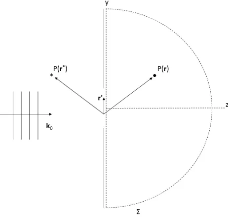
3.2 Geometry for Scalar Diffraction (Kirchoff) Integral. . . 46

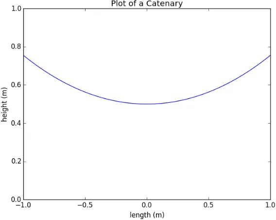
3.3 Plot of a catenary. . . 59

3.4 Plot showing the normalized 2D RCS of a circular cylinder for various radii at normal incidence. The noisy signature at the end was caused by machine precision errors which arose when too many terms were used for the calcula-tion. Physical optics would be the preferable method in this high-frequency regime. The kk and ⊥⊥ subscripts refer to incident and outgoing TM and TE modes, respectively. . . 61

3.5 Depiction of the orientations of the polarization basis vectors from the air-craft’s frame of reference (H and V polarizations) and the powerline’s frame of reference (TE and TM polarizations). The definitions shown above were used to convert the polarization amplitudes from one frame to another. . . 63

(10)

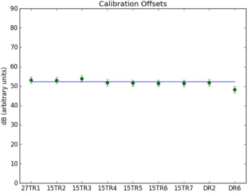
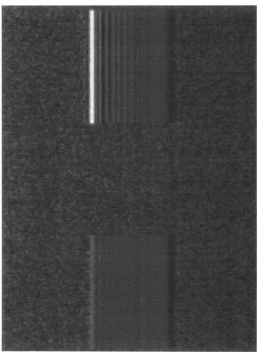
4.1 Process imagery for Gotcha collection. (a) Total power image of AFRL data produced employing RITSAR using all 360◦ of azimuth for backprojection processing. Canonical targets appears as point sources in the top-left por-tion of the image. (b) Image of view for which powerlines were apparent in the upper-right portion of image. . . 68 4.2 Locations of canonical targets in the scene provided by AFRL/SNA [5]. . . 69 4.3 Plot showing the calibration offsets calculated using each of the canonical

targets. Although the targets were of different sizes and types and placed at different orientations, the calculated offsets were very similar. The range of the plot matches the range of the intensity scale for the raw image. The mean value indicated by the blue bar represented the actual offset used. . . 71 4.4 Flight paths used to collect the AFRL data for all 8 passes. . . 73 4.5 Screen shot of Blender scene used for DIRSIG simulation. . . 74 4.6 Depiction of the anechoic chamber setup from the Michigan experiment [6]. 76 4.7 Image showing calibration sphere placed on top of mount [6]. . . 77 4.8 Image showing powerline placed on top of mount [6]. . . 78 4.9 Images depicting the geometric cross-section of each object for which RCS

measurement were made: (a) 1.27 cm cylinder (b) 167.8 MCM Copper (c) 556.5 MCM Aluminum (d) 954 MCM Aluminum & Steel and (e) 1431 MCM Aluminum & Steel. All cables were ≈1 ft in length [6]. . . 79 4.10 Image chip of isolated transmission lines. . . 80 4.11 Picture taken of a representative telephone pole configuration. The actual

telephone pole only had three transmission lines on top, configured similarly to what is shown in the picture, as well as a thick bundle of communication cables halfway up. Images of the actual telephone poles could not be obtained. 81 4.12 Physical model images. (a) Sketch of powerline in CAD software (b) 3D

powerline plot (c) Side view of the top transmission line. . . 82

5.1 Qualitative Image Comparisons: (top) AFRL Gotcha, (bottom) simulated. . 85 5.2 Intensity histograms for grassy field showing noise characteristics of data.

A good fit using a Rayleigh distribution was obtained for both the simu-lated DIRSIG data and the Gotcha field data. This is consistent with the noise distribution expected for coherent imaging modalities. (left) DIRSIG simulated, (right) Gotcha. . . 86 5.3 RCS plots for trihedral targets: (a) TR1 (b) TR2 (c) TR3 and (d) TR4.

(11)

LIST OF FIGURES 10

5.4 RCS plots for trihedral and dihedral targets: (a) TR5 (b) TR6 (c) DR2 and (d) DR6. The target labels TR5-DR6 correspond to those in figure 4.2.The DIRSIG derived RCS’s consistently underestimate the observed re-turn, likely due to the absence of a physical optics capability. This effect is especially pronounced for the dihedral targets which have small accep-tance angle in elevation. Also absent in the simulated dihedral RCS’s are sidelobes, which require physical optics to be modeled. . . 89 5.5 View of finite cylinder at different aspects, as measured from plane normal

to axial direction: (a) 0◦ (b) 20◦ (c) 40◦ (d) 80◦. Note the increasing view of the endcap and decreasing view of the cylindrical portion. . . 92 5.6 Modeled X-band power line RCS compared to anechoic chamber

measure-ments for 1.27 cm diameter (ka = 2.5) smooth cylinder: (top-pair) using Physical Optics and Physical Theory of Diffraction exclusively (bottom-pair) using exact smooth cylinder 2-D diffraction coefficient for cylindrical portion and PO/PTD for endcaps (left-pair) HH channel (right-pair) VV channel. Error bars on the measured data are scaled by ±1 standard de-viation. For the simulated data, error bounds depict the O(k·a)−1 error associated with using a stationary phase technique to evaluate the contour integral along the edge adjoining the endcap and cylinder. . . 93 5.7 Modeled X-band power line RCS compared to anechoic chamber

measure-ments for 167.8 MCM (ka= 2.4) copper power line: (top-pair) using Physi-cal Optics and PhysiPhysi-cal Theory of Diffraction exclusively (bottom-pair) us-ing exact smooth cylinder 2-D diffraction coefficient for cylindrical portion and PO/PTD for endcaps (left-pair) HH channel (right-pair) VV channel. Error bars on the measured data are scaled by ± 1 standard deviation. For the simulated data, error bounds depict theO(k·a)−1error associated with using a stationary phase technique to evaluate the contour integral along the edge adjoining the endcap and cylinder. . . 94 5.8 Modeled X-band power line RCS compared to anechoic chamber

(12)

5.9 Modeled X-band power line RCS compared to anechoic chamber measure-ments for 954 MCM (ka= 6.1) steel & aluminum power line: (top-pair) us-ing Physical Optics and Physical Theory of Diffraction exclusively (bottom-pair) using exact smooth cylinder 2-D diffraction coefficient for cylindrical portion and PO/PTD for endcaps (left-pair) HH channel (right-pair) VV channel. Error bars on the measured data are scaled by ±1 standard de-viation. For the simulated data, error bounds depict the O(k·a)−1 error associated with using a stationary phase technique to evaluate the contour integral along the edge adjoining the endcap and cylinder. . . 96 5.10 Modeled X-band power line RCS compared to anechoic chamber

measure-ments for 1431 MCM (ka= 7.0) steel & aluminum power line: (top-pair) us-ing Physical Optics and Physical Theory of Diffraction exclusively (bottom-pair) using exact smooth cylinder 2-D diffraction coefficient for cylindrical portion and PO/PTD for endcaps (left-pair) HH channel (right-pair) VV channel. Error bars on the measured data are scaled by ±1 standard de-viation. For the simulated data, error bounds depict the O(k·a)−1 error associated with using a stationary phase technique to evaluate the contour integral along the edge adjoining the endcap and cylinder. . . 97 5.11 Modeled C-band power line RCS compared to anechoic chamber

measure-ments for 1.27 cm diameter (ka = 1.3) smooth cylinder: (top-pair) using Physical Optics and Physical Theory of Diffraction exclusively (bottom-pair) using exact smooth cylinder 2-D diffraction coefficient for cylindrical portion and PO/PTD for endcaps (left-pair) HH channel (right-pair) VV channel. Error bars on the measured data are scaled by ±1 standard de-viation. For the simulated data, error bounds depict the O(k·a)−1 error associated with using a stationary phase technique to evaluate the contour integral along the edge adjoining the endcap and cylinder. . . 99 5.12 Modeled C-band power line RCS compared to anechoic chamber

(13)

LIST OF FIGURES 12

5.13 Modeled C-band power line RCS compared to anechoic chamber measure-ments for 556.5 MCM (ka = 2.2) aluminum power line: (top-pair) using Physical Optics and Physical Theory of Diffraction exclusively (bottom-pair) using exact smooth cylinder 2-D diffraction coefficient for cylindrical portion and PO/PTD for endcaps (left-pair) HH channel (right-pair) VV channel. Error bars on the measured data are scaled by ±1 standard de-viation. For the simulated data, error bounds depict the O(k·a)−1 error associated with using a stationary phase technique to evaluate the contour integral along the edge adjoining the endcap and cylinder. . . 101 5.14 Modeled C-band power line RCS compared to anechoic chamber

measure-ments for 954 MCM (ka= 3.0) steel & aluminum power line: (top-pair) us-ing Physical Optics and Physical Theory of Diffraction exclusively (bottom-pair) using exact smooth cylinder 2-D diffraction coefficient for cylindrical portion and PO/PTD for endcaps (left-pair) HH channel (right-pair) VV channel. Error bars on the measured data are scaled by ±1 standard de-viation. For the simulated data, error bounds depict the O(k·a)−1 error associated with using a stationary phase technique to evaluate the contour integral along the edge adjoining the endcap and cylinder. . . 102 5.15 Modeled C-band power line RCS compared to anechoic chamber

measure-ments for 1431 MCM (ka= 3.5) steel & aluminum power line: (top-pair) us-ing Physical Optics and Physical Theory of Diffraction exclusively (bottom-pair) using exact smooth cylinder 2-D diffraction coefficient for cylindrical portion and PO/PTD for endcaps (left-pair) HH channel (right-pair) VV channel. Error bars on the measured data are scaled by ±1 standard de-viation. For the simulated data, error bounds depict the O(k·a)−1 error associated with using a stationary phase technique to evaluate the contour integral along the edge adjoining the endcap and cylinder. . . 103 5.16 Qualitative Image Comparisons: (left) AFRL Gotcha (right) simulated

(top) platform at top-right (bottom) platform at bottom-left. . . 105 5.17 Quantitative RCS Comparisons: (left) HH channel (right) VV channel (top)

platform at top-right (bottom) platform at bottom-left. . . 107 5.18 Image chip of isolated transmission lines when the platform was at (a)

top-right and (b) bottom-left of image. Four distinct signals are apparent in the latter image even though only three transmission lines were observed on the telephone pole (plus the already accounted for single bundle of com-munication wires). This was observed for all 8 passes. . . 109 5.19 RCS Comparisons assuming no sag: (left) HH channel (right) VV channel

(14)

4.1 AFRL platform parameters used for the DIRSIG simulation. . . 72

4.2 Material reflectivity parameters used for the DIRSIG simulation. . . 75

5.1 X-band results summary. . . 98

5.2 C-band results summary. . . 104

5.3 AFRL Gotcha results summary. . . 108

(15)

List of Major Symbols

a Powerline diameter.

d 2D diffraction coefficient. For backscattering from an infinitely long, perfectly conduct-ing 1D object, This quantity is also equal to the Incremental Length Diffraction Coefficient.

D 3D diffraction coefficient.

Ei Incident field, oriented along the polarization direction.

Es Scattered field, oriented along the polarization direction. k wavenumber.

k wavevector.

k·a wavenumber-diameter product.

Ψ Obliquity angle of incident/scattered radiation, measured from plane perpendicular to the powerline’s axial direction.

β Obliquity angle of incident/scattered radiation, measured from the powerline’s axial direction.

R Distance from receiver to target.

R Distance from receiver to target, oriented along propagation direction.

r Distance from a point on the powerline to a scene reference point.

σ Radar Cross Section.

(16)

Detecting powerlines is an important remote sensing application. The information gleaned from power line detection can be used to characterize an area’s power infrastructure. It can also be used in hazard avoidance applications for low flying aircraft. In both cases, a potential application can be found in humanitarian relief for natural disasters. Specifically, having the ability to remotely sense powerlines can give decision-makers a quick survey of the damage to a power grid over a wide area. It can also aid pilots of low flying search-and-rescue aircraft in mission planning. In the optical regime, powerlines do not often exhibit a strong return due to their smallness and the radiometry of the problem. In the radar regime, however, powerlines can be a very prominent feature in the processed imagery for certain viewing geometries. Since the diameter of a typical power line is often on the order of only a few wavelengths for radar, a significant portion of the return is due to diffraction.

This research focused on modeling the radar return from power lines. There are nu-merous benefits that result from having an accurate model for powerline returns. One benefit is the ability to determine if a conceptual system will be able to perform pow-erline detection given the system’s operating parameters, such as carrier frequency and flight path. This benefit gives program managers the ability to predict if a given system design can meet certain mission requirements with regards to powerline detection, avoid-ing significant hardware expense. Similarly, a second benefit would be to determine if an existing system can perform the mission given its operating parameters. The enhanced capability of a space-borne SAR system, for example, would illustrate this benefit. If the model predicts powerline detection will be more effective on one pass than another, this information can be used by mission planners to optimize the sensor’s tasking. Finally, a model of the powerline return for an existing system and operating parameters can be used to determine an a priori matched filter for post-processing on actual data. This is a

(17)

CHAPTER 1. INTRODUCTION 16

common application for forward modeled data.

There has been much work recently on the development of software which simulates the SAR signal for large urban scenes. An overview of the research in this area performed to date is provided in Chapter 2. In particular, an experimental capability has been added to the Digital Imaging and Remote Sensing Image Generation (DIRISIG) tool for the radar imaging modality [7]. DIRSIG is a tool widely used in the Electro-optic/Infra-red (EO/IR) modalities which produces radiometrically accurate, physically based imagery [8]. DIRSIG is shown to simulate the SAR phase history for a given scene and operational parameters and is unique to other software tools that have the same focus on modeling the SAR signal for complex scenes. There is also a plethora of tools available for modeling the Radar Cross Section of an object. One popular example is Xpatch [9], a tool used by the Air Force research labs which uses the Shooting and Bouncing of Rays (SBR) technique. Unfortunately, as will be explained later, SBR does not perform well for optically thin objects such as powerlines at typical radar wavelengths. One effort made by Sarabandi, K. [4] resulted in a Method of Moments (MoM) approach for the specific purpose of modeling powerline RCS’s. At millimeter-wave frequencies, evaluation of the source current integral was simplified by making a physical optics approximation. However, this approximation breaks down for wavenumber-diameter products.1. All previous work considered, a gap is apparent for efficiently yet accurately modeling the radar return of powerlines in this regime.

A brief overview of the methods used to model the scattering of Electromagnetic (EM) waves is provided in Chapter 3. This chapter begins by reviewing how a RCS is defined. The RCS of an object describes how efficiently it scatters radiation given its shape, material properties, the viewing angle, and the angle of incidence of the incoming radiation. The remainder of Chapter 3 reviews the different ways to calculate how an object scatters EM radiation, with a concentration on how diffraction is modeled. As mentioned earlier, the dominant scattering mechanism by powerlines is due to diffraction. Diffraction is a phenomenon that describes how electromagnetic radiation scatters off obstructions. This phenomenon is most readily observed when the characteristic length of the scattering object is on the order of a few wavelengths. In the case of powerlines, typical diameters are on the order of a few to tens of centimeters. Since the wavelength of radiation in the radar regime is also typically on the order of a few centimeters, diffraction becomes the dominant scattering mechanism.

(18)

geometric properties. The powerline was assumed to be a perfectly conducting smooth cylinder with sag described by a catenary. The two dimensional problem for scattering into the forward cone was then solved to yield a 2D diffraction coefficient. A 3D diffrac-tion coefficient was then derived using the ILDC approach developed by Mitzner. This 3D coefficient was then used to generate both powerline RCS’s that were later compared to experimentally measured RCS’s. The 3D diffraction coefficient was also used to generate a SAR phase history. The scene resulting from this phase history was then compared to an actual circular SAR collection from the Air Force Research Labs (AFRL) [5].

The methods used to validate this ILDC approach are described in Chapter 4. First, a generic assessment of DIRSIG’s radar modality was performed. The scene used for the DIRSIG simulation roughly matched that of the AFRL field collection and included pow-erlines and canonical targets such as dihedrals and trihedrals. The parameters used for the simulation closely matched what was provided in the AFRL auxiliary data. The assess-ment included not just an investigation of whether or not DIRSIG could model powerlines, but also how well it performed against the canonical targets. Additionally, DIRSIG’s abil-ity to simulate the noise present in a SAR image was assessed. Next, the ILDC approach for generating 3D diffraction coefficients for powerlines was validated against data taken in an anechoic chamber by the University of Michigan [6]. Included in this discussion is a description of how the experiment was setup and calibrated. Finally, the simulated powerline phase history was compared to that observed in the field-measured AFRL data [5]. The method used to perform this comparison is also provided.

(19)

Chapter 2

Background

The methods used to simulate SAR imagery are significantly different from those used to simulate EO/IR imagery. For those most familiar with how a traditional optical system works, the most striking difference is the way in which an image is formed. In conventional optics, the spatial aperture collecting the signal is two dimensional. For SAR, the spatial aperture is the one-dimensional flight path of the platform. The temporal length of the received signal forms the second dimension. The time domain signal, before demodulation, is a measurement of the phase of the electric field. This is unlike conventional optics where a detector element usually measures power, which is proportional to the time average of the electric field squared. Since SAR systems measure and record the phase of the electric field, signal processing needs to be applied to form an interpretable image. This signal processing is usually done at the hardware level or in post-processing. This is in contrast to how an image is formed in optics, where the physics of light propagation does all of the signal processing. For example, in a single lens system, the phase of the electric field across the aperture is mixed with the lens thickness function and is then matched filtered by the Fresnel convolution kernel. All of this signal processing is transparent to users of traditional optical imaging systems.

The variability of signal processing methods that can be used to process SAR data presents difficulties for methods attempting to simulate SAR imagery, using conventional Fourier optics. Measurements made by SAR systems are further up the imaging chain than that of optical systems. For a SAR system, the measurement of the phase of the electric field is made at the aperture level, whereas for traditional optics, measurements are made after “Fresnel post-processing” and measuring the time average of the electric field squared. As a result, the system transfer function of a SAR system is more complex and also much more customizable than that of a traditional optical system. Once an optical system is built, the impulse response usually remains static. For SAR systems, the

(20)

impulse response can change from one collection to another, based on a variety of factors. These include, but are not limited to, the length of the flight path, the characteristics of the transmitted signal, and the different kinds of reconstruction algorithms that were applied to the recorded phase history. Additionally, since the reflectivity of a target can vary greatly across the length of the SAR aperture, applying a shift-invariant impulse response to a reflectivity map can lead to inaccurate results. For example, the impulse response of a perfect point reflector will be much different from the point spread function (PSF) for a point reflector which has a small acceptance angle. Along azimuth, the spatial frequency region of support for the perfect reflector will be determined by the length of the full synthetic aperture, whereas the target with the low acceptance angle will be smeared in azimuth, since only a fraction of the full aperture will have contained signal.

In addition to the differences in the image formation process, there are other more subtle differences between conventional EO/IR and radar imaging modalities. Since SAR involves coherent illumination of the target area, speckle is the dominant source of noise. Speckle is observed when the amplitude of the surface roughness is on the order, of or less than, a wavelength and the correlation length across the surface is much less than a resolution cell. When these conditions are met, the observed intensity of a single resolution cell is determined by a sum of impulse responses with random phases [11].

Effects due to diffraction are also more pronounced in SAR since radar wavelengths are longer than EO/IR wavelengths. Early SAR simulators modeled diffraction effects in SAR imagery in a statistical sense, similar to how speckle is modeled [3]. This worked fairly accurately at low resolution [3]. As the resolution of SAR systems has increased in recent years, the need to use more accurate diffraction models has increased [3]. This is especially important in urban scenery where narrow streets can act as wave guides, rectangular structures can produce unattended diffractions, and strong scattering from man-made surfaces that have edges or corners can dominate the return signal [3].

(21)

CHAPTER 2. BACKGROUND 20

Later versions of the tool could model multiple scattering by using geometric optics for all but the final bounce back to the receiver. Physical optics was then used to calculate the scattered field on the final bounce.

GRECOSAR and SARAS are examples of code that have been specifically written to simulate the SAR phase history for a given scene. Some examples of software tools traditionally used for modeling in the optical regime that have been adapted for SAR simulation are POV-RAY [2] and DIRSIG [7, 8]. One of the effects commonly seen in urban imagery is displacement of a signal due to multiple bounce returns. This effect manifests itself when a pulse bounces multiple times before finally coming back to the receiver. Since the range of the pulse is determined by the time of flight, the signal is often located farther downrange than the actual location of the last position the pulse was scattered from. This can lead to reduced image interpretability. Ray-tracers such as POV-RAY have been used to create efficiently images which replicate the effect of multiple bounces, but are otherwise radiometrically inaccurate. The intended use of this program is to aid analysts in interpreting SAR imagery which contain large, complex structures. Another tool adapted to simulating SAR imagery is DIRSIG. While DIRSIG is a mature and widely used tool for producing radiometrically accurate imagery in the EO/IR regime, its radar modality is still experimental at this stage. DIRSIG takes the geometric optics approach to modeling the return signal and does not incorporate physical optics or any other high-frequency technique. The signal is built up on a pulse-by-pulse basis by convolving the transmitted pulse with delta functions centered at the time of flight of each ray shot into the scene. The result is a tool which is efficient, models multiple scattering, and accounts for targets with dynamic, aspect-dependent reflectivities, but is limited by the geometric optics approximation.

For achieving a very high degree of accuracy, the computationally intensive Finite Difference Time Delay (FDTD) [3] method has also been used. Due to the complexity of this approach and the stringent hardware requirements needed for implementation, simulations have been limited to simple objects commonly found in urban scenery. While this method would be too complicated to use for modeling a complex scene given current hardware capabilities, it has value in obtaining high fidelity results for simple, common objects.

(22)

problem was further simplified for periodic structures, such as helically wound cables found in powerlines. In such cases, a periodic Green’s function could be used to calculate the scattered field from the source currents. This requires only one period (or helix pitch for powerlines) for the analysis rather than the entire structure. It was demonstrated that this technique could accurately model the Bragg scattering peaks observed in measured data at a frequency of 94 GHz.

Finally, the Xpatch® toolkit is worth mentioning. Xpatch is a ubiquitous radar mod-eling tool that has a number of capabilities. For estimating source currents, it uses the Shooting and Bouncing of Rays (SBR) technique. This technique requires a high-frequency assumption. Consequently, it will not provide accurate results for surfaces whose wavenumber-diameter product is.10. This includes typical powerlines at X-band frequencies and lower.

2.1

GRECOSAR

The Graphical Electromagnetic Computing (GRECO) tool is a graphical modeling tool which computes the RCS of a target [12] using a variety of high-frequency techniques. These include Physical Optics, Method of Equivalent Currents, Physical Theory of Diffrac-tion, and Impedance Boundary Condition (IBC) techniques.

Processing the RCS of a target begins with creating a 3D CAD model of the target. An image of this target, as viewed from a given observation point, is rendered onto a workstation’s screen by the graphics hardware. Assuming a monostatic collection, each pixel on the screen corresponds to a point illuminated by the incident radiation. All other target points are assumed to be in the shadow region and, according to high-frequency approximation techniques, do not contribute to the RCS. Typically for RCS modeling, the target’s surface is broken up into a series of facets and wedges. GRECO is unique in that it describes a target using parametric surfaces. For each target pixel rendered, the position x, y, z and surface normal nx, ny, nz components are derived by using non-uniform rational B-splines (NURBS) for interpolation [18]. Once the surface parameters are derived for each illuminated point in the image, the CPU performs the electromagnetic scattering computation.

(23)

CHAPTER 2. BACKGROUND 22

discontinuities in the surface normal. For a given wedge angle, incidence angle, and po-larization, there is a corresponding diffraction coefficient. Diffraction coefficients act in much the same way as reflection coefficients as they relate the incident field amplitude to the scattered field amplitude for a given geometry and polarization. A more detailed discussion of diffraction coefficients is provided in 3.2.7. The line integral along the edges is then computed by summing the contributions from each edge pixel. Results shown in [12] demonstrated a high degree of accuracy when compared to numerical solutions. Using only physical optics, accurate RCS’s for non-stealth targets could be obtained.

GRECOSAR is a code that uses GRECO to compute the RCS of objects in a given scene and simulates the SAR signal [13]. For each azimuth position, an image of the scene from the viewpoint of the platform is rendered. GRECO computes the frequency dependent RCS in the frequency domain. This response is applied to the time domain signal by means of an inverse Fast Fourier Transform along the range dimension.

The GRECO code has been exhaustively validated for both canonical and complex targets [14]. GRECOSAR is relatively experimental but has been used in studies to evaluate SAR images of fisheries [13] and individual naval vessels [14]. In the literature [13, 14], much of the phenomenology observed in real world scenarios was captured by the simulator [15]. Recently, GRECOSAR’s ability to model urban scenes has also been evaluated. The study was mostly limited to an image of a box of gypsum on top of a perfectly conducting plane. While examples of GRECOSAR’s ability to model more complex urban scenes has not been found in the literature, initial results for easily validated simple scenes were promising [15].

2.2

SARAS

The Synthetic Aperture Advanced Simulator (SARAS) is code that generates the raw SAR signal using a physical optics approach [16]. The form of the physical optics integral for backscattering, discussed later, is given by [16]:

Es(R) =

ikexp (−ikR) 4πR E0

I−kˆkˆ

·F(ˆn)

Z

A

exp (2ik·ρ)dA (2.1)

(24)

this method results in strict sampling requirements. One way to avoid this is to create facets whose characteristic length is much larger than the correlation length and to use an approximation for the re-irradiation diagram. Possible approximations include cosδ, cos2δ, and exp

h −_δδ

0

i

whereδ is the angle between the line-of-sight and surface normal and δ0 is given by the user. More accurate, numerical solutions can also be used for the

irradiation diagram. For theF(ˆn) term, the height of the facet vertices is approximated by assuming a normal distribution about the mean height. and a deviation from the nominal surface normal is derived using these modified vertex positions. This results in speckle in the observed image, as expected for coherent illumination of stochastic surfaces.

Once Es has been computed for each facet, a derived parameter referred to as the reflectivity map γ(x, y) is calculated for each facet location. The value of γ(x, y) is equal to the amplitude of the field scattered by a small area centered on (x, y), divided by that area and the incident field amplitude [1]. The quantity Es can be calculated based on a single bounce assumption [16] or account for multiple bounces [1]. As shown in the literature [1], accurate results can be obtained by using geometric optics for all but the last bounce, at which point physical optics (eq. 2.1) is used for the final propagation step to compute the field scattered back to the receiver.

After calculating the reflectivity map γ(x, y), the raw signal is built up assuming a transmitted linear FM signal. Defining a temporal variablet0 =t−tn−2R_c0 wheretis the fast time and tn is the slow time, the heterodyne signal is computed using the following formula:

h

x0 =vt,r0=

ct0

2

= Z Z

γ(x, y)·g(x0−x, r0−r;x, r) (2.2)

where

g(x0−x, r0−r;x, r) =w2

x0−x X

rect

r0−r cτ /2

exp (iφ) (2.3)

φ=−4π

λ ∆R+ α

2

t0−2r

c −

2∆R c

2

(2.4)

and w is the illumination footprint. Noting that equation 2.2 represents a convolution, efficient calculation of the raw signal can be performed via the Fast Fourier Transform and filter theorem:

H(ξ, η) =G(ξ, η)Γ(ξ, η) (2.5)

where the capital letters represent the Fourier transform of the respective lowercase terms in 2.2 and (ξ, η) represent the spatial frequencies of the azimuthal and range coordinates, (x, r), respectively.

(25)

CHAPTER 2. BACKGROUND 24

[image:25.612.214.401.268.522.2]

the dihedral. Returns from dihedral structures, such as where a wall intersects with the ground, appear bright in SAR imagery due to multiple bouncing of rays. For wall-ground intersections, the wall can be approximated as a smooth surface with a strong specular component predicted by physical optics, whereas the ground can be approximated to first order as having a random surface height about some mean [19]. In work done by Franceschetti, these approximations were used to model the multiple bouncing of rays from urban structures [1]. The resulting SAR imagery, shown below, exhibited many effects one would expect from a dihedral return such as a bright return from the corner and higher order returns farther along the range direction.

Figure 2.1: Image of two buildings with different material properties generated using SARAS. Higher order wall-ground reflections are apparent for both buildings [1].

(26)

2.3

POV-Ray

In a paper by Stefan Auer et. al. [2], a distinction is made between SAR simulators that focus on radiometric quality and those that focus on geometric quality. The previously mentioned simulation tools, GRECOSAR and SARAS, are examples of algorithms that focus on radiometric quality. These computationally intensive algorithms are limited by the level of detail allowed for the 3D models [2]. For scenes that contain complex geo-metrical structures, using an approach that sacrifices radiometric accuracy for geometric accuracy may be preferable. The software package used in the work by Auer et. al. [2] was POV-Ray, an open-source ray tracing algorithm. Examples given in the literature [2] include modeling the scattering from the Wynn Hotel and the Eiffel Tower, shown below:

[image:26.612.145.469.293.528.2]

(a) (b)

Figure 2.2: (Left) actual and (Right) simulated images of the Wynn Hotel. Special features in each image are labeled with corresponding letters [2].

Modeling with POV-Ray begins by creating a model of the scene. Illumination is simulated with a cylindrical light source. This approximation does not account for 1/r4

(27)

CHAPTER 2. BACKGROUND 26

are called secondary rays. The contribution from each bounce is weighted by a reflection coefficient. For the sake of simplicity and to reduce computational complexity, the surface reflectance was modeled as lambertian with a specular lobe. Next, the contributions from each ray are mapped to an azimuth and range coordinate. For each secondary ray, an additional ray is created that is parallel to the primary ray but travels in the opposite direction from the intersection point back towards the camera. The intersection of this additional ray with the camera is labeled the ray origin. The azimuth coordinate in the image plane is calculated by taking the mean value of the azimuth coordinate for the ray’s origin and the azimuth coordinate for the ray’s pixel location. Range is derived from the depth value of the intersection point. The final output of the system is a reflectivity map of the scene in azimuth and range coordinates. This output is obtained by superimposing a rectangular grid over the irregularly spaced returns from each ray and performing an interpolation step.

Simulations were made on a skyscraper, the Wynn Hotel, and the Eiffel Tower. In many cases the brightness of the reflectivity map did not match well with the actual data. This was especially the case along building edges where a significant diffracted return would be expected, or at locations on the building’s surface that contained dihedrals/trihedrals not modeled by the smoothed version in the ray tracing simulator. The main utility, however, was to be able to classify features in the reflectivity map by the number of bounces and the macroscopic structures from which the signal was scattered. This improved image interpretability, as it identified why some features present in the SAR imagery, were absent from traditional overhead imagery taken by a camera.

2.4

DIRSIG

The Digital Imaging and Remote Sensing Image Generation (DIRSIG) tool is a physics-based ray-tracing algorithm used to model imagery across the electromagnetic spectrum for remote sensing applications [8]. Its ability to produce radiometrically accurate images for single-band, multi-spectral, and hyperspectral modalities is very well established. DIRSIG also has a mature LIDAR modeling capability [8]. DIRSIG’s ability to model SAR imagery is still experimental at this stage. No work has been done that validates DIRSIG’s SAR simulation capability.

(28)

addi-tion of these techniques adds another layer of computaaddi-tional complexity, especially when imperfectly conducting surfaces or higher-order bounces are involved.

Modeling in DIRSIG starts with the creation of a scene. Scenes are usually built in the ray tracing software Blender and a .ODB file is created. For each object ID in the scene, the material properties are specified in a .mat (material) file. The next step is to specify the pertinent system parameters and viewing geometry. For a traditional DIRSIG simulation, this can usually be done through a Graphical User Interface (GUI). To date, all of these parameters have to be provided in xml tables as specified in the DIRSIG SAR Modality Handbook [7]. DIRSIG then models the SAR return on a pulse-by-pulse basis. For a given pulse, particles are shot into the scene from the transmitter using the LIDAR package. In single-pass mode, the receive computations are performed in the same pulse simulation as the transmitted one. In two-pass mode, a hit map is created from the intersections, stored to file, and a separate simulation is run for the receive computations. Using two-pass mode lessens numerical noise [7]. For each return, the transmitted waveform is convolved with a delta function delayed by the time-of-flight. The fast-time signal for a given pulse is then created by summing each of the returned waveforms. The amplitude of each return is also scaled by the Fresnel reflection coefficients. This is repeated for each pulse until the entire time domain phase history for the user-defined collection is obtained.

(29)

CHAPTER 2. BACKGROUND 28

2.5

FDTD

Many of the approaches discussed thus far involve a high-frequency approximation for the incident field. In geometrical optics, this approximation is applied to the Luneberg-Kline series. As shown in section 3.2.2, only the first term of this series is taken as a solution to Maxwell’s equations in the high-frequency limit. This results in an eikonal equation which leads to the well known laws of reflection and refraction, as well as an additional equation that accounts for amplitude loss with propagation and polarization effects. The Geometrical Theory of Diffraction and Uniform Theory of Diffraction are extensions of Geometrical Optics that describe how rays interact with edges, curved surfaces, and with themselves, for example at a caustic. In physical optics, the high-frequency approximation leads to an assumption that non-uniform currents near an edge or shadow boundary can be neglected. In both physical optics and the physical theory of diffraction, asymptotic forms of diffraction integrals are acquired by making a high-frequency approximation. This permits form solutions for diffraction coefficients without having to compute an integral for each differential diffracting element.

All of the high frequency techniques above are only approximate solutions to Maxwell’s equations. All of these approximations become less accurate at low frequencies. Many of them also do not take into account internal propagations [3] such as physical optics, which assume source currents are constrained to the surface. Obtaining an exact solution to Maxwell’s equations can be practically impossible for arbitrary surfaces where the boundary conditions are difficult to implement in a natural coordinate system. In such cases, where high-frequency techniques are insufficient, and exact closed form solutions cannot be obtained, numerical techniques are frequently used. The two most common techniques are the Method of Moments [17] and Finite Different Time Delay (FDTD) [21]. The FDTD algorithm works by sampling a scene with a Yee lattice [21], creating a source, then modeling propagation by differencing the field in adjacent cells for a given time step, as specified by the scalar rectilinear components of Maxwell’s curl equations. Boundary conditions are imposed by specifying the behavior of certain cells. For example, for a point on the surface of a conductor, the tangential E-field components are always 0. The main drawback to this algorithm is the sampling requirements. In [3], the spatial sample spacing used was ₁₀λ. Even for manageable scene sizes, the temporal resolution requirements often result in thousands of time steps [3].

(30)

[image:30.612.146.468.242.495.2]

common objects in an urban scene. One of the canonical problems investigated was how perfectly conducting plates, with smooth or rough surfaces, scattered radiation. For the smooth surface, the backscattered signal was dominated by diffraction peaks along the edges, whereas for rough surfaces, the signal was dominated by a speckle pattern which appeared across the surface. The statistics of the speckle pattern followed a Rayleigh dis-tribution, as expected [3]. Below is a plot showing the field amplitude for both a smooth and rough plate:

Figure 2.3: Simulated amplitude of field reflected from both a smooth and rough plate using FDTD [3].

(31)

CHAPTER 2. BACKGROUND 30

2.6

Millimeter-wave Physical Optics Model

At Ka-band frequencies and higher, Bragg scattering features can be observed in a pow-erline’s RCS [22]. This is due to the fact that powerlines are normally comprised of a number of cable strands which are tightly wound in a helical structure, which are peri-odic in nature. At certain aspect angles, adjacent rays reflected from this periperi-odic surface constructively interfere, leading to multiple orders of peaks in the RCS signature. The locations of these peaks are given by [4]:

θn= sin−1

nλ

2L (2.6)

[image:31.612.100.516.395.604.2]

Wherenis an integer,θis the aspect angle measured from a plane normal to the powerline’s axial direction, λand 2L is the length of one period. The phenomenon that causes these peaks is the same as the one that gives rise to the Bragg diffraction pattern observed when x-rays are scattered from a periodic crystal lattice. Sarabandi, K. and Moonsoo, P. developed a way to compute the scattered field from powerlines using a method that accounts for Bragg scattering [4]. This method uses an accurate powerline geometrical model, shown below:

(32)

The tangential component of the total magnetic field on the surface of the powerline in-duces source currents. These source currents can be computed from the incident magnetic field using an integral which can be evaluated numerically via the Method of Moments (MoM). The MoM is a technique which provides accurate results but is computationally intensive at higher frequencies [4]. In order to efficiently evaluate the source current inte-gral without having to use MoM, a high-frequency approximation was made. This allowed the source currents to be computed using a perturbation series instead of MoM. The 0th order term in the series was the usual physical optics current given byJ0(r) = 2 (n×Hi). Higher order terms were computed from this 0th order approximation using the pertur-bation series approach. The resulting nth order physical optics current was then used to compute the scattered field using Green’s theorem. For periodic structures, a periodic Green’s function was used and only one period of the powerline was needed for calculat-ing the scattered field. For non-periodic structures, such as powerlines with a significant amount of sag, the normal free space Green’s function was used and the entire lit portion of the powerline was needed for calculation instead of just one period.

(33)

[image:33.612.145.466.94.343.2]

CHAPTER 2. BACKGROUND 32

Figure 2.5: Simulated versus experimental RCS’s at 94 GHz for 4 different powerlines in the VV channel. Bragg scattering peaks were accurately modeled by a PO approach at millimeter wavelengths [4].

One of the primary drawbacks to using a physical optics approach is that the high frequency approximation breaks down at X-band frequencies and lower for typical pow-erline diameters. Additionally, physical optics does not account for the VV contribution from the grooves observed in experiment [4, 6] and predicted by theory [23]. While the use of MoM becomes more tractable for modeling powerline RCS’s at lower frequencies, it would still be difficult to implement this for a SAR application involving thousands of pulses. For non-periodic powerline geometries with an appreciable amount of sag, the MoM approach would require calculations to be performed across the entire surface of the powerline as opposed to just one period. This would include the non-lit regions for lower frequencies. Consequently, hardware requirements could be hard to fulfill for existing commercial off-the-shelf desktops.

2.7

Xpatch

(34)

is modeled using a Shooting and Bouncing of Rays (SBR) technique. As will be discussed later in section 3.2.6, SBR is a high-frequency method which uses ray tracing to predict source currents on a facet-by-facet basis. These source currents are then used to calculate the contribution to the scattered field from the surface of a facet using physical optics (assuming far-field observation) and the contribution from an edge using PTD. In order for SBR to work, either the size of the facet has to be large enough or the bundle of rays has to be dense enough for the incident field to be adequately sampled. This may not be practical for optically thin wires or powerlines. Being a high-frequency technique, SBR is also susceptible to errors in cases where the radius of curvature of the wire is too small. Generally, this is considered to be the case when the wavenumber-diameter product, k·a, is .1 which is where this research is focused.

2.8

Summary

The techniques for simulating SAR imagery and RCS’s presented here each have unique capabilities. Examples of code that have been developed for the express purpose of being a SAR simulator are GRECOSAR and SARAS. Software traditionally used for modeling imagery in the EO/IR regime such as DIRSIG and POV-RAY have also been adapted for efficient modeling in the radar modality. While computationally intensive, FDTD has also been used to calculate the scattering from canonical targets for simple scenes, materials, and geometries. With respect to modeling powerlines, a physical optics based approach was established for millimeter-wave radiation. Xpatch is another tool commonly used for radar modeling. This tool relies on SBR, a high-frequency approximation technique. Unfortunately, SBR breaks down for wavenumber-diameter products which are .10.

(35)

Chapter 3

Theory

In this chapter, a discussion that focuses on the different ways to model electromagnetic interactions with matter are presented. At a top-level, an object’s RCS is often used to describe how well the given object scatters power incident on its surface. The RCS is a function of wavelength, angle of incidence, angle of observation, and the object’s material and geometric properties. It can be derived from the radar range equation, which relates the power transmitted by an antenna to the power received at an antenna after the incident radiation has scattered off an object. The RCS can also be expressed in terms of a ratio of the squared magnitude of the fields incident on the surface and scattered from the surface, as measured in the far-field. This latter definition enables the RCS to be computed from first principles. This chapter begins with a formal definition of the RCS and then moves to a discussion of the different ways to model how objects scatter electromagnetic radiation. Once traditional methods for modeling electromagnetic scattering have been reviewed and a common terminology established, the method used in this research to model power-line scattering is presented. This effort began with the creation of a physical model which defines the geometric and material properties of the powerline. Once these were estab-lished, the 2D problem of scattering into the forward cone (defined by Fermat’s principle for Edge Diffraction, section 3.2.3) was solved. Work done by Mitzner [10] relates the 2D solution to the 3D scattering problem. It was shown that the 3D diffraction coefficient can be expressed as a function of an Incremental Length Diffraction Coefficient (ILDC). For the special case of backscattering, this ILDC is equal to the 2D diffraction coefficient. Once the ILDC-based method for calculating the 3D diffraction coefficient was established, a number of follow-on activities were enabled. This included the simulation of powerline RCS’s as well as the quad-polarization phase history for a SAR collection.

(36)

3.1

Radar Cross Section Definition

The radar range equation is commonly used to assess how well a given set of operating parameters for a radar system can meet mission requirements. It relates the transmit-ted power to the received power through various loss and gain terms. The radar range equation, as defined in Ruck’s RCS Handbook, is given below [24]:

Pr=

PtGt

Lt

| {z } T ransmitting

system

1 4πr_t2Lmt

| {z } P ropagating medium σ |{z} T arget 1 4πr2_L

mr

| {z } P ropagating

medium

Grλ20

4πLr

| {z } Receiving system 1 Lp

| {z } P olarization

ef f ects

(3.1)

where [24],

Pt= transmitter power in watts

Gt= Gain of the transmitting antenna in the direction of the target

Lt= numerical factor to account for the losses in the transmitting system

Lr= a similar factor for the receiving system

rt= range between the transmitting antenna and the target

σ= radar cross section

Lmt, Lmr= numerical factors which allow the propagating medium to have loss

r= range between the target and receiving antenna

Gr= gain of the receiving antenna in the direction of the target

λ0 = radar wavelength

Lp = numerical factor to account for polarization losses

When the transmitter and receiver are located on separate platforms, the collection ge-ometry is termed bi-static. When the transmitter and receiver are co-located (r=rt), the collection is termed mono-static. Of particular interest for this research is the σ term in equation 3.1. This is the RCS of the target. The RCS is a commonly used metric that describes how efficiently an object scatters radiation. Rearranging the range equation and solving forσ yields the following expression [24]:

σ= 4πr2 4πPrLmrLp λ2₀Gr | {z }

power density scattered f rom

target

/ PtGt

4πr_t2LtLmt | {z } power density

at target

(37)

CHAPTER 3. THEORY 36

The equation above is useful for measuring the RCS of a target in a lab. When calculating the RCS of a target from first principles, however, it is often more convenient to express

σ as a function of the incident and scattered fields rather than power. The power density of electromagnetic radiation, W, is given by the following expression [25]:

W =Z0(E·E∗)/2 (3.3)

WhereZ0 is the impedance of free space andE is the electric field vector (oriented along

the polarization axis). Substituting this expression for the braced terms in equation 3.2, an alternate way of calculating σ is as follows:

σ = 4πr2(E

s_·_Es∗₎

(Ei·Ei∗) = 4πr

2(Hs·Hs ∗₎

(Hi·Hi∗) (3.4) where the i and s superscripts refer to incident and scattered fields, respectively. At first glance, the equation above implies that the RCS is a function of distance. This is often undesirable since a more useful target metric would be one that is independent of the receiver distance and is solely dependent on target properties. One can achieve such a metric by first noting the quantity (Es·Es∗) falls off as 1/r2 in the far-field [25]. Consequently, the more widely used definition of the RCS, which does not depend on receiver distance, is given as follows:

σ = 4π lim r→∞r

2(Es·Es ∗₎

(Ei·Ei∗) = 4πrlim→∞r

2(Hs·Hs ∗₎

(Hi·Hi∗) (3.5) One way of interpreting this result is that σ can be thought of as “the area intercepting the target that, when scattered isotropically, produces at the receiver a density that is equal to the density scattered by the actual target” [24]. Importantly, σ describes how efficiently a target scatters power but does not provide any insight into how a target affects the phase of the scattered field. Since SAR systems measure the phase of the scattered field, this will become important later on when methods for modeling how radiation is scattered from a power line are discussed.

3.2

Modeling Electromagnetic Propagation

(38)

modeling of scattering from more complex objects using Maxwell’s equations, however, is often too difficult to do analytically. The main issue with complex objects is the difficulty one has in applying boundary conditions to the scattering surface in a natural coordi-nate system. Numerical methods such as Finite Difference Time Delay (FDTD) [21] and Method of Moments (MoM) [17] can be used for more complex surfaces. The drawback to these methods is the spatial and temporal sampling requirements become onerous if the scene becomes too large or too complex [3]. Usually, approximations for the solutions to Maxwell’s equations need to be made. One such approximation is geometric optics (GO), the basis for essentially all ray tracing models. While GO does not fully take into account the wave nature of light, one can attach to each ray a ”payload” that keeps track of polar-ization, amplitude, and phase information as the ray travels through space and interacts with objects. In this way, one can account for some of the effects associated with the wave nature of light such as interference and polarization dependent reflection coefficients. GO works well when the wavelength of light is much smaller than the characteristic length of the object. This approximation does not work well for describing how rays scatter off of features such as edges, tips, curved surfaces with small radii of curvature, and caustics. A solution is to use the Geometrical Theory of Diffraction (GTD) developed by Keller [27]. GTD essentially uses exact methods to determine ray amplitudes and what Keller describes as Fermat’s Principle for Edge Diffraction to determine all the possible ray paths (and consequently, phases) for a given geometry.

(39)

CHAPTER 3. THEORY 38

the surface can be segmented into local tangent planes.

In both GTD and PO, a singularity arises when computing the scattered field from shadow boundaries for certain surfaces. Ufimtsev’s Physical Theory of Diffraction (PTD) [28] corrects this by subtracting the scattered field due to uniform currents (those predicted by PO) from the fields predicted by more exact solutions (GTD and the Sommerfield solution for scattering from a half plane), to obtain the scattered field solely due to non-uniform currents. The difference in the GTD and PO singularities is finite [25]. The main limitation with PTD is it only predicts the scattered field in what is termed the Keller cone [25], defined by Fermat’s Principle for edge diffraction [27]. For scattering directions outside the Keller cone, an extension of PTD developed by Mitzner which uses Incremental Length Diffraction Coefficients (ILDC’s) can be used [25, 10].

The approximations to Maxwell’s equations described here are termed high frequency approximations. They are labeled as such since a high frequency approximation is made to either neglect higher order terms in the Luneberg-Klein series solution to Maxwell’s equations (Geometric Optics) or to obtain analytic approximations for diffraction integrals using a steepest descent or stationary phase method. While the wavelength of radar is much longer than that at optical regimes, these high frequency techniques still yield accurate results for many applications [25]. The main drawback to these techniques, however, is their inability to account for surface traveling (creeping) waves easily [25]. While GTD makes allowance for these creeping waves, it does so only for simple shapes. Even with simple shapes, however, it is still possible for a creeping wave to make many revolutions around a closed surface, emitting radiation as it travels along. These higher order emissions drastically increase the computational complexity. Efficiently modeling the scattering due to creeping rays is an area of ongoing research [25].

(40)

coeffi-cients), and wavelength of radiation. A very similar approach is taken by the Shooting and Bouncing of Rays (SBR) technique [31, 32]. In this method, rays incident on a surface can come from both the source as well as from secondary reflections from other objects in the scene. Once the rays have propagated, the surface currents are approximated assuming plane wave incidence and a PO integral is evaluated to yield the final result.

3.2.1 Maxwell’s Equations

With very few exceptions, solutions to Maxwell’s equations represent the most accurate model for how electromagnetic radiation interacts with matter. The more accurate the-ory of Quantum Electro-Dynamics is usually more applicable to light-matter interaction problems such as scattering from single atoms at resonant frequencies, the photo-electric effect, and in the case of very strong fields, vacuum polarization resulting from electron-positron pair creation [33]. This research will investigate how light interacts with relatively macroscopic objects whose work functions are much greater than the energy contained in a radar-wavelength photon. Consequently, the solutions to Maxwell’s equations will be considered the most accurate for the purposes of this research. Maxwell’s equations are given as follows:

∇ ·E= ρ

0

(3.6)

∇ ·B= 0 (3.7)

∇ ×E=−∂B

∂t (3.8)

∇ ×B=µ0j+

1

c2 ∂E

∂t. (3.9)

While Maxwell himself did not derive the four equations above, he is credited with having recognized that they result in a wave equation:

∇2E− 1

c2 ∂2E

∂t2 =

1

0

∇ρ+µ0 ∂j

∂t (3.10)

∇2B− 1

c2 ∂2B

∂t2 =µ0∇ ×j. (3.11)

In the absence of free charge and current (ρ=j= 0), equations 3.10 and 3.11 transform into the vector Helmholtz equation:

(41)

CHAPTER 3. THEORY 40

with k₀2 = ω2/c2. The equations above can be solved by resolving the fields into their vector components and solving the resultant scalar equations. Under certain constraints, the resulting scalar equations result in the scalar Helmholtz equation:

∇2₊_k2 0

ψ(r) = 0 (3.14)

where aneiωt is suppressed andψ(r) is a scalar field that can be related to the fieldsE,B, or as shown later a vector potential A, by a vector a such that E,B,A=aψ(r). One of the constraints required to go from the vector Helmholtz equation to the scalar Helmholtz equation is propagation through isotropic media, a condition automatically satisfied in free space. The other constraint is on the choice of the direction of a with respect to the coordinate system used for the Laplacian operator ∇2_{. In rectangular coordinates,} _a_can

be in any arbitrary direction [34]. In a spherical coordinate system, a must point in the radial direction [34]. For a cylindrical coordinate system,a must lie along the z-axis [34]. In other words, analysis is restricted to TEz and TMz modes. This may seem restrictive at first glance. However, given that the TE and TM modes form an orthogonal basis and the incident and scattered fields in radar applications are usually linearly polarized, solutions can be obtained by decomposition of the fields into the two basis vectors. When acannot be chosen to lie along one of the system’s coordinates, solutions to the scalar Helmholtz equation can still be used but specifying the boundary conditions becomes exceedingly difficult. One example of scattering by a surface specified in prolate spheroidal coordinates is given in [35]. In that paper,awas chosen to lie along one of the rectangular coordinates (TEx, for example). The incident field, originally specified in rectangular coordinates, had to be decomposed into a sum of spheroidal wavefunctions so that the boundary conditions in that coordinate system could then be specified and the solution for the scattered field obtained.

On the assumption the problem can be reduced to solving the scalar Helmholtz equa-tion, Green’s theorem can be used to transform the problem into an integral equation. A well known example of this in the field of optics is shown later in section 3.2.4. Another approach is to assume the solution is separable into three orthogonal coordinatesξ1, ξ2, ξ3:

ψ(ξ1, ξ2, ξ3) =ψ1(ξ1)ψ2(ξ2)ψ2(ξ2) (3.15)

For propagation through free-space, the solution is given as follows:

ψ(x, y, z) =ψ0e[i(kxx+kyy+kzz)] (3.16)

Another example is propagation through a rectangular waveguide. In this case, boundary conditions need to be imposed, mainly that the field goes to 0 along the walls of the rectangular prism. The result is a solution which has discrete wave numbers:

ψp,q(x, y, z) =ψ0e

h

i

pk0x+qk0y+

√

1−p2₋_q2_zi

(42)

where p and q are integers.

For infinitely long cylinders, the problem can be reduced to two dimensions by ex-amining the solution at some point along the cylinder’s axis. In polar coordinates, the two-dimensional Helmholtz equation can be written as [36]:

∇2+k2

f = 1

r ∂ ∂r r∂f ∂r + 1 r2 ∂2f ∂θ2 +k

2_f _{= 0}_. _(3.18)

Since we are working in cylindrical coordinates, f represents solutions for TEz or TMz modes. After separation of variables with f = R(r)Θ(θ), and choosing −m2 to be the separation constant for theθcoordinates, solutions to the polar two-dimensional Helmholtz equation are of the form [36]:

ψm(r, θ) =

∞

X

m=0

[amcos(mθ) +bmsin(mθ)]Zm(kr) (3.19)

whereZm is any function that satisfies Bessel’s ODE [36]

r2 d 2

dr2Zm(kr) +r d

drZm(kr) + (k

2_r2₋_m2₎_Z

m(kr) = 0 (3.20) Functions that satisfy the above ODE are Bessel functions of the first kind Jm(kr), Neu-mann functions Nm(kr), and Hankel functions Hm(kr) [36]. Any linear combination of these functions that satisfies the boundary conditions for a given problem may be used. The boundary conditions also specify the coefficients am and bm. This will become im-portant later in section 3.3.2 when the scattering of electromagnetic waves from cylinders is examined in detail.

3.2.2 Geometric Optics

One of the most common high frequency approximations to Maxwell’s Equations is that of Geometrical Optics (GO). This approximation is also referred to as ray optics. Using this method, light propagation is modeled using bundles of rays that emanate from a source and interact with objects. The direction of a ray is governed by Fermat’s principle. Applying conservation of energy to a tube of rays yields amplitude information. Mathematically, GO is derived from the Luneberg-Kline series solution to the Helmholtz equation [34]:

E(R, ω) =e−ik0ψ(R) ∞

X

m=0

Em(R)

(iω)m (3.21)

(43)

CHAPTER 3. THEORY 42

1. Eikonal Equation

k∇ψk2 =n2 (3.22)

2. Transport Equations

∂E0 ∂s +

1 2

∇2_ψ

n

E0 = 0 (3.23)

∂Em

∂s +

1 2

_∇2_ψ

n

Em =

vp 2 ∇

2_E

m−1 (3.24)

m= 1,2,3. . . (3.25)

3. Conditional Equations

ˆ

s·E0= 0 (3.26)

ˆ

s·Em=vp∇ ·Em−1 (3.27)

m= 1,2,3. . . (3.28)

where ψ is a surface which describes the wavefront, n is the index of refraction, s is the ray distance, and ˆs is normal to the wavefront ψ. The geometric optics approximation is represented by the 0th order term. This is called a high-frequency approximation since higher order terms in the Luneberg-Kline series, equation 3.21, are assumed to be negligi-ble. Equations 3.22 and 3.26 together are a representation of Fermat’s Principle, or more specifically, Snell’s law and the law of reflection. Taking the first term of equation 3.21 and substituting into the transport equation 3.23 yields the following result [34]:

E(s) = E0₀(0)eiφ0(0)

| {z } Field at reference

point (s=0)

r _ρ

1ρ2

(ρ1+s)(ρ2+s)

| {z }

Spatial attenuation (divergence, spreading) factor eiks |{z} Phase factor (3.29)

whereρ1 andρ2are the radii of curvature of the wavefront at some reference s= 0 andφ0