The impact of university degrees on the lifecycle of earnings : some further analysis

(1)

BIS RESEARCH PAPER NO. 112

THE IMPACT OF UNIVERSITY DEGREES ON THE LIFECYCLE OF EARNINGS: SOME FURTHER ANALYSIS

(2)

Report prepared by Ian Walker and Yu Zhu on behalf of the Department for Business, Innovation and Skills

Authors: Professor Ian Walker (University of Lancaster) and Yu Zhu (University of Kent)

The views expressed in this report are that of the authors and not necessarily those of the Department for Business, Innovation and Skills or any other Government Department.

Department for Business, Innovation and Skills 1 Victoria Street

London, SW1H 0ET

(3)

Executive summary

This report, commissioned by the Department for Business, Innovation and Skills (BIS), provides further evidence on the impact of higher education on lifetime net earnings. There are two important components to the research: the statistical modelling of the relationship between higher education and gross earnings (and employment) that is used to predict

what non-graduate earnings (and employment) would have been if only they had been graduates; and then simulating the way in which taxes and the student loan scheme affect these predicted gross earnings to allow us to infer the relationship between higher

education and net earnings.

While earlier BIS research has focussed on the marginal effect of qualifications our focus is to compare the earnings (and employment) of those individuals who have a first degree (and 2+ A-levels) with those with 2+ A-levels and no higher education degree –

irrespective of the subsequent qualifications of both sets of individuals. We think of this as capturing the decision-making of young people thinking about the prospective futures. While previous research has been based on the large Labour Force Survey (LFS)

datasets, here we also exploit the British Household Panel Survey (BHPS) data - both in isolation and in conjunction with LFS. LFS has information on degree class and degree subject – the “major”. BHPS contains information on HEI type (Russell Group, etc), slightly better data on A-Level qualifications and some family educational background information. Neither dataset contains both sets of information, so exploiting both is helpful. Our

estimates suggest larger impact of lifetime gross earnings than previous research has. We simulate the predicted earnings (and employment status) of individuals in our data and then average these to show that the private benefit of a degree, in terms of lifetime

(6)

Key Findings

 Our estimate of the return to a degree relative to 2+ A-levels but no degree, defined by the coefficient on this variable in a regression model of earnings, is 23% for men and 31% for women. These are comparable to the findings of other research.

 We estimate that there are very substantial effects of a degree on the net present value of the lifecycle of incomes: our best estimates of the likely impact on

discounted lifecycle net earnings of having a degree, relative to not having a degree, is 28% for men (approximately £168k) and 53% for women (approximately £252k) on average.1 While our estimates of the average effect of a degree on earnings and the probability of employment suggest that previous estimates are robust to a number of criticisms, previous work fails to capture an important difference between graduates and non-graduates in the trend growth in real wages. It is this that counts for much of the difference between our estimates relative to previous research.

 Our estimates for a good degree (first or upper second) are significantly larger than for lower degree classes (by £76k for men and £85k for women, on average) suggesting a large return to student effort. Allowing for the effects to vary with family background suggest no significant differences.

 We attempt to identify dropouts by comparing age left education with age associated with highest qualification and find that male HE dropouts earn approximately the same as individuals who never attended HE. For females we find that there is a small wage penalty – dropping out from HE is worse than never attending HE. However, controlling for dropouts makes little difference to our conclusion about the graduate premium.2

 We find estimates of the effect broken down by degree subject that support earlier research - but we are not, with available data, able to test the robustness of these estimates. This is a matter of concern since there are grounds for thinking that some of the differences across subjects are a reflection of differences in the students rather than differences in curriculum – for example, the A-level admission requirements might be different across subjects. Research elsewhere has also been uninformative on this issue.

1_{These figures are simulations of lifecycles of earnings from a statistical model of gross earnings and are}

adjusted for tax and National Insurance liabilities, periods of non-participation, and for the effect of the loan scheme, and discounted at 3.5%.

2_{Our control group has 2+ A-levels. Relatively few such students go on to Further Education (FE). So we do}

(7)

 We extend earlier research to consider the effect of degree by type of higher education institution. While we do find significant differences in a simple specification, we find that these differences are smaller and become statistically insignificant when we include some basic family background controls that capture at least some of the differences across students. Thus, our research does not suggest that there are large differences in returns across broad types of HEI, controlling for background.  One focus for our work is to untangle the effects of cohort (of birth) from age and

calendar time. There are two reasons we are interested in doing this. First, over time, there has been a growth in the gap between graduate and non-graduate wages in many countries. Second, we are also interested in exploring cohort differences

associated with the rapid and large expansion of HE in the late 1980s and early 1990s. We are particularly interested in the extent to which the expansion of HE that occurred then might have reduced the impact of a degree on earnings. We compare the

earnings of young graduates and non-graduates pre and post the HE expansion but find no significant differences in the graduate earnings differentials associated with the expansion of HE.

 We extend earlier research on the net present value of the net impacts of a degree in a number of ways that turn out to be economically significant. In particular, we simulate the impact of a degree on the whole distribution of earnings rather than just simulate the average effect. This allows us to capture the extremes of the data - graduates who do better than average pay more higher rate tax than would otherwise be thought; and graduates who do worse than average repay less of their student loans than would otherwise be thought. Simulating the effect on the average predictions for graduate and non-graduate earnings distribution tends to underestimate the net present value associated with HE relative to what we find when we simulate each individual and then average these simulated effects.

 We find that the new higher tuition fees make a predictable difference to the present value relative to previous fee levels. However, we also find that the recent changes to the loan system insulates students who come from low income households from much of the effect of higher tuition fees.

(8)

1. Introduction

This report, commissioned by the Department for Business, Innovation and Skills (BIS), provides further evidence on the impact of higher education on lifetime net earnings. It attempts to extend, verify, and refine the work conducted in 2011 by Gavan Conlon and Pietro Patrignani of London Economics for BIS that was published as “The Returns to Higher Education Qualifications”, BIS Research Paper 45 (hereafter referred to as LE). One aspect of the extensions to earlier work is to investigate how higher education impacts across parental background, and how type of higher education attended affects lifetime earnings.

Like LE, we consider both the relationship between higher education and earnings, and with employment. There are two important components to the research: the statistical modelling of the relationship between higher education and gross earnings (and

employment) that is used to predict what non-graduate earnings (and employment) would have been if only they had been graduates; and then simulating the way in which taxes and the student loan scheme affect these predicted gross earnings to allow us to infer the relationship between higher education and net earnings. LE’s evidence, while

comprehensive, begged a number of questions. While LE provides a very detailed

breakdown of the aggregate results by subject studied, it left unanswered questions, such as: the effect of higher education institution (HEI), the effect of obtaining a degree through part-time study, and the effect of obtaining a degree later in life as opposed to immediately after leaving schooling at the age of 18.

While we provide further evidence to LE in some of these areas, where data are available, we are also (deliberately) more restrictive in other ways. In the main, this reflects a

philosophical difference between this work and LE. LE focusses on the marginal effect of qualifications. That is, they compare the earnings of individuals with a particular vector of qualifications with the earnings of individuals with a different vector. For example, they compare the earnings of individuals with 2+ A-levels and a first degree (but not

subsequent higher education qualifications) with the earnings of individuals with 2+ A-levels but with no further qualifications above A-level, to yield the marginal effect of a first degree. And, they compare the earnings of individuals of those with a first degree and a Masters degree (but no further qualifications) with those with a first (Bachelor) degree alone, to yield the marginal effect of a Masters degree. And so on. In contrast, our focus is to compare the earnings (and employment) of those individuals who have a first degree3 (and 2+ A-levels4) with those with 2+ A-levels and no higher education degree –

irrespective of the subsequent qualifications of both sets of individuals. We think of this as capturing the decision-making of young people thinking about the prospective futures. At the age of 18 (or later), entering higher education offers the option of further HE

qualifications beyond a first degree. And, not entering higher education offers the option of further study, perhaps undertaken part-time and/or on-the-job, that might yield additional

3_{Unlike LE we do not consider higher education qualifications that are at sub-degree level (they are in our}

“2+ A-level “control” group rather than in the “treatment” group) but the proportions are small so the effect on our results is insignificant. We treat Foundation Degrees the same as first degrees. They account for a very small proportion of graduates and excluding them, or treating them separately, make no effective difference to our analysis and findings.

(9)

qualifications – which may be professional, vocational or technical. That is, our philosophy is to capture the option values associated with the decision made to attend higher

education or not.

How the work reported here differs from LE is explained in more detail in Section 2. This section explains the methodology and, in particular, what is novel in what we do relative to previous research. Section 3 briefly reviews the finding of existing work – and more detail of UK research can be found in LE. Rather than repeat the review in LE, we focus on literature that relates to the extensions to the LE work that we try to implement. We also highlight some of the caveats that apply to research of this type and explain how one might examine the robustness of the results to these caveats. This section considers not only the statistical modelling but also the simulation analysis.

Section 4 explains the selection of our datasets, and describes the characteristics of the sample used in our subsequent analysis. While previous UK research has been based on the large Labour Force Survey (LFS) datasets, here we also exploit the British Household Panel Survey (BHPS) data - both in isolation and in conjunction with LFS. LFS has

information on degree subject – the major. BHPS contains information on HEI type (Russell Group, etc). But neither dataset contains both sets of information. So exploiting both is helpful. Section 5 presents results for earnings conditional on being employed and for the probability of employment. In Section 6 we exploit these results to provide the simulated lifecycles and the implications for individuals and the exchequer. Finally, Section 7 concludes with recommendations for further research.

In anticipation of our detailed results we find broadly similar results to LE when we confine ourselves to broadly similar specifications. In particular, the estimate of average effect of a degree on gross hourly earnings seems only slightly lower than that found by LE. Our results, for a specification that is similar to LE, suggests that a degree adds about 22% (33%) to male (female) hourly earnings (compared to LE estimates of 24% (31%)). To get a feel for what this implies in pure financial terms, note that 22% over and above the average annual male earnings for those with 2+ A-levels but no degree of approximately £30,000 p.a. is, over a working lifetime of 40 years, a little over one-quarter of a million pounds at current prices not discounted. Similarly for women, 33% of an average of

approximately £21,000 pounds p.a. for 40 years is also a little over one-quarter of a million pounds. Of course, there are costs: tuition fees, additional subsistence, and the lost

earnings during higher education. Moreover, the progressive income tax system will reduce this large apparent return. So, too, will discounting future incomes to make them comparable with the current costs incurred while studying. On the other hand, allowing for employment effects of higher education will make this return larger because, on average, graduates experience less unemployment and non-employment than non-graduates. All of these issues are factored into our more detailed work below.

(10)

[image:10.595.69.465.105.385.2]

Figure 1 Headline estimates of average discounted lifetime NPVs of graduate earnings differentials (£k): WZ vs LE

0 50 100 150 200 250 300 WZ LE G ra dua te di sc ount e d ea rn in gs d if fer en ti al , £, 000 Men Women

While we have searched for evidence that recent cohorts of graduates enjoy a smaller earnings premium over non-graduates, we have not found any statistically significant differences. Our suspicion is that a smaller graduate earnings premium may have been driven by the rapid and large expansion in the supply of graduates that occurred in the early 1990s. If this exceeded the expansion in the demand for graduates then we would expect that increasing competition for graduate jobs would lead to a fall in the graduate earnings premium. If this were the case then it might reasonably be regarded as a long term effect – until rising demand caught up with the higher HE participation rate. But a second possibility is that a lower earnings premium for recent graduates is a cyclical phenomenon arising from them entering a labour market that was suffering from

recession. If this were the correct explanation then we might reasonably expect any low earnings premium for recent graduates to be a temporary phenomenon. Unfortunately, we do not yet have sufficient data on the earnings history of young graduates who graduated in the early 1990s and beyond to be able to say whether what we might observe is

because HE participation had increased dramatically or because the recession resulted in unemployment rising from 6.9% to 10.7% between 1990 and 1993 which depressed the market for new graduates by more (or less) than other workers. This will only be resolved in time as we get more earnings history for the expansion graduates in the post-recession period.

Finally, we have the advantage over LE in that we can now provide simulations of the effects of new tuition, scholarship and loan arrangements because we now know what has been implemented. Here, we show, amongst other things, that studentships and the

(11)

2. Methodology

This section considers a wide variety of issues that arise in this literature. Prominent amongst these are: identifying lifecycle effects separately from time and cohort effects; selection into work; selection into higher education; and selection into subject of study.

2.1 Gross earnings for employees over the lifecycle

There is a long history of research that attempts to understand the distribution of earnings as the result of the investment decisions that individuals make in their human capital. The essence of the theory of human capital is that it is formed by investing – in education. If the capital market works efficiently then the return on an investment in a degree should be the same as the return on any other similar financial investment – call this rate r. If the

proportionate gain in earnings associated with an investment in a degree is (w1-w0)/w0 , where w1 is the earnings5 for an individual with a degree (D=1) and w0 is for the individual without (D=0), then this should differ from r only by some random amount e whose value on average would be 0. The proportional difference in earnings is (approximately) the difference in the log of earnings.Thus, the theory suggests that log w1 - log w0 = rD + e. And if log w0 depends linearly on a vector X of other characteristics like sex, region, etc., so that log w0 = α + X’β, then we can write the log of earnings for any individual as

log w = α + X’β + rD + e

whereβ is a vector of parameters associated with the variables X, such that X’β is the sum of each of the products of each of the X’s and their corresponding β’s. Thus, αis the log wage of a default individual (with sex=0, region=0, etc) without a degree and α + r is the log wage of the default individual with a degree. That is, the earnings differential

associated with a degree is (approximately) r . And this is the same for all individuals regardless of X because the effects difference out when we subtract the expected non-graduate earnings from the expected non-graduate earnings.6 _{The use of log earnings as the} dependent variable is suggested by the theory and has the useful implication that the coefficients on the explanatory variables can be interpreted as percentage effects: thus, if the coefficient on D were 0.10 then we would infer that earnings for observations with D=1

were, on average, 10% higher than those for D=0. Similarly if the coefficient on sex (being male, say) were 0.2 then we would infer that, other things being equal, men would be 20% better paid than women on average.

This very simple (log) linear specification explains the variation in log earnings across individuals by the differences in their X’s, whether they have a degree or not, i.e. D, and a random component, e, that captures the unobserved factors that influence w0. The X

vector is usually specified to include a measure of work experience to capture the accumulation of human capital that occurs on-the-job through training and learning by doing. This is often incorporated as a quadratic function of age. Age is a proxy for

5_{We use hourly earnings throughout our empirical analysis.} 6_{Strictly speaking}_{r = log w}

1 - log w0 ≈(w1 - w0 )/ w0and the approximation is fairly accurate for values of r

(12)

experience (which is often not observed in many datasets) and the quadratic relationship derives from a presumption that learning on the job is subject to diminishing returns - the older one gets the less easily one learns. It is this (assumed) quadratic shape that drives the lifecycle of earnings.

Such an equation has become the workhorse model for empirical research in the

determination of earnings. There are many estimates of such models and it is this basic framework that is used in the work by LE. However, the derivation of this relationship depends on a variety of assumptions made for convenience. The theory has strong

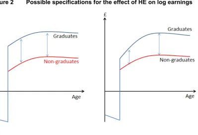
implications that may not be borne out in practice. For example, this specification assumes that the effect of having a degree is the same for all values of X. In particular, the model implies that age earnings profiles are parallel in D - having a degree simply shifts the (log) earnings quadratic pattern vertically upwards. That is, the simple specification assumes that log earnings for graduates and non-graduates conforms to the left panel in Figure 2 – that age - log earnings profiles are parallel. This is a strong restriction and one that is usually rejected by the data when a model such as that in the right panel of Figure 2 is estimated. Indeed, it is common to find that log earnings differentials between graduates and non-graduates are narrower at an early age, as shown here. Similarly, the left hand side of Figure 2 assumes that the impact of any of the X’s, for example sex, is the same for those with D=1 as those with D=0. This is a strong restriction but one that is seldom tested. It is easily rejected here in favour of a specification where we allow all coefficients on the X’s to differ with D. Thus, a preferable model is one where the wages of graduates are allowed to be determined differently than the wages of non-graduates: in other words, by the two equations written as

log wD = αD + X’βD + eD , where D = 0,1.

Thus the log wage differential associated with having a degree is now (α1 + X’β1) – (α0 +

X’β0_{). Since (}_α1 _–_α0_{) =}_r_{this can be rewritten as}_r₊_X’(_β1_–_β0₎_{which makes it very clear} that the log earnings differential associated with a degree is now allowed to vary with X if

β1 and β0 differ. Thus, a test of the general specification against the restricted

specification, as in LE, is that β1₌_β0 _{for all the coefficients in the model. This has typically} been strongly rejected in the literature.

Thus, our methodology is an important extension of earlier work. However, it has the disadvantage that it does not yield a single number to summarise the effects of a degree. Rather there will be an estimate for each cell of the X matrix.7_{However, to arrive at an} aggregate figure we only have to take the weighted average for each cell.

7_{In practice, the number of cells is quite small – here, for each sex, we group the data into six regions, two}

(13)

[image:13.595.76.476.88.361.2]

Figure 2 Possible specifications for the effect of HE on log earnings

2.2 Cohort

effects

There have been considerable changes in the Higher Education (HE) system in the UK over the last 40 years. We have moved from an HE system that was provided for a small elite, free of tuition fees with mean-tested grants for subsistence, and so was highly subsidised. We have moved to a system where a large minority of any cohort attends HE, there are much smaller direct tuition subsidies and an extensive and sophisticated system of income contingent loans which are heavily subsidised, and grants in the form of income contingent bursaries and (academic) merit based scholarships. Differences across

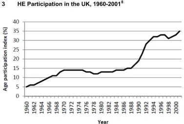
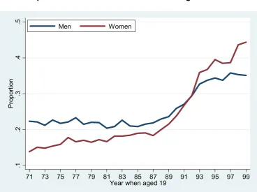
devolved governments have also emerged. Moreover, there have been large changes in the supply of graduates to the labour market - Figure 3 shows the dramatic increase in HE participation rates that occurred from the late 1980s until the mid 1990s. It seems likely that this dramatic growth has affected the distribution of wages – post expansion cohorts may well experience smaller degree differentials than pre-expansion.

A major concern for us is to capture the lifecycle variation in log earnings. However, we have a strong reason for suspecting that age affects earnings not just through work

experience but also through year of birth. For example, this large expansion in the number of graduates in the labour market that began in the early 1990s may well have driven down the graduate earnings premium. This is a cohort effect: the earnings that you receive at any age depend independently on whether you graduated into a labour market where graduates were scarce (before the expansion) or when they were plentiful (afterwards). Distinguishing between lifecycle, cohort, and time effects is important for our purposes. There is productivity growth over time and the literature has strongly suggested that this productivity growth is “skill biased” – that is, it is higher for skilled workers (graduates) than unskilled (non-graduates). There are changes in HE participation across cohorts that give rise to cohort effects in earnings that differ between graduates and non-graduates. Finally, there is the pure lifecycle growth in earnings that we need to account for in order to

(14)

[image:14.595.93.471.84.339.2]

Figure 3 HE Participation in the UK, 1960-20018

If we were using just cross section data taken in a particular year then the age of each individual would be the survey year minus the year of birth. So year of birth and age would be perfectly collinear and it would not be possible to identify the age earnings profile

except by assuming that there were no independent cohort effects driven by year of birth. This would be a very strong assumption. Repeated cross sections allow us to separate out any TWO of these effects assuming the third is zero. The LFS data provide cross sections from 1993 to 2010 which can be pooled together (adjusting wages for inflation) but even this would present us with a collinearity problem to an extent. As an alternative to this we can exploit the fact that LFS is a short panel – wages are recorded in waves 1 and 5, a gap of one year. Thus, we could exploit the wage growth recorded in the panel data to estimate the age earnings profile for workers.

There is a selection issue here – individuals could only be included in this analysis if they record earnings in both waves 1 and 5, while the alternative would only require that we

8_{There have been two official measures: the Age Participation Index (API) for all Great Britain up to 2000,}

(15)

observe wages in either wave. On the other hand, the usual cross section method makes the implicit assumption that age (minus the age at which you ceased education) and experience are one and the same thing, so it ignores spells of non-participation that might occur. This is a useful approach because it exploits the LFS data to its full. The LFS is a panel of addresses not people. So researchers need to drop observations in the panel where the wave 1 household members are not present in wave 5 – for example, the whole family may have moved. Thus, the dataset used for the first step is a subset of the dataset used for the second step.

On balance we prefer exploiting panel data to estimate age-earnings profiles because the estimates derive from the effects of one year of work experience on earnings. That is, we think of the age variable (and its square) as capturing the effects of work experience on earnings. For men, age is a good proxy for (unobserved) work experience but for women, especially women from early cohorts, it is not because of interrupted spells of work

associated with childcare. Thus, estimating the lifecycle of earnings from the cross section data we would be likely to underestimate the effect of experience from the effect of age, for such women. But, by confining attention to individuals who are observed in successive years in a panel we can attribute the earnings growth to the effect of experience between successive interviews.9 Thus, the first step of the two step method allows us to estimate the way in which earnings evolve over the lifecycle.

To see, more precisely, how this two-step method works assume, for simplicity, that X contains only age and age squared. Our model of earnings determination would then be

log witD = αD + ηD.Ageit+ γD. Ageit2+ eitD

where the i subscript indicates individual i and eitD captures the effect of all unobservable factors that we cannot control for using our data - for example, ability and ambition. Then we can use the panel data to form a wage growth equation obtained by taking the equation above, that shows wages at time t, and subtracting from it the same equation at t-1 to obtain

Δlog witD = ηD+ 2γD. Ageit +ΔeitD

where Δ is the time difference operator (that is, Δlog witD = log witD - log wit-1D), to allow us to estimate γD and ηD from a wage growth equation in a first step. Notice that this equation is unaffected by any cohort differences IF the only effect of cohorts was captured by αDin the first equation. It is possible to estimate the lifecycle parameters, ηD and γD, from panel data. These parameters can then be fixed in the second stage, where the equation for the level of wages, log witD, is estimated. This fixes the lifecycle component of wage variation and allows the cohort variation to be captured independently.

The assumption underlying this is that cohort effects do not affect the shape of the age earnings profile.10_{But they can independently affect the height of the profile. So, once we} have estimates of γD and ηD from the panel data we can impose these estimates on to the cross section data and estimate the remaining parameters, including any cohort effects. Thus, if αD, which determines the height of the age-earnings profile, varies across

9_{LE report that they estimate their log hourly earnings equation in five year age intervals. In addition they}

also report that they include age and age squared. This is more general than our specification – which effectively collapses the five intervals into one. We tested whether including age interval dummy variables were jointly significant when age and age squared where included and found that they were not.

(16)

individuals in a way which depends on one’s cohort (i.e. if we allow αiD =αD(cohorti)) then we can write log earnings as

2

ˆ ˆ

D - D D (D )

it it i i i

log w  Age  Age   cohort eD

where a “hat” above a coefficient indicates that it has been estimated (in the first step). We could then estimate how αD depends on i’s cohort (defined by year of birth) by applying linear regression to this equation using the cross section data in a second step. As in the first step, we can estimate separate equations for degree holders (D=1) and others (D=0) in this second step. We refer to this procedure as our two-step model: in the first step we use the panel to estimate the lifecycle parameters, γD and ηD, for each group, D=0,1; and in the second step we estimate the remaining parameters (on the other X’s) including the cohort and calendar time11 effects – again for each group.

In practice, we divide the data into three groups: the oldest cohort was born before August 1970 and so reached the usual age to attend university on or before the 1989 intake which is prior to the expansion period; the second cohort were born between September 1970 and August 1976 and so will have typically started university during the expansion period; while the third cohort were born after August 1976 and so attended university after 1995 when the rapid expansion was coming to an end.

It seems reasonable to suppose that this large and rapid expansion in the supply of

graduates to the labour market will have forced down the earnings of graduates. However, Walker and Zhu (2008) were not able to find statistically significant effects of the

expansion of higher education. It remains to be seen whether the arrival of more post expansion data since that earlier research will allow us to make more precise estimates.

2.3 Employment, Non-Employment, and Self-Employment

Naïve economic theory suggests that wages in competitive labour markets are determined by productivity alone. In such circumstances, market forces equilibrate demand and supply for all types of worker such that unemployment is eliminated quickly. However, there are many reasons for thinking that labour markets do not work very efficiently and that unemployment occurs as an equilibrium phenomenon. Thus, there may be a case for thinking that education affects not just wages but also the probability of being in

employment. Therefore, like LE, we model the probability of being in employment similarly to log wages. However, just as in our approach to modelling earnings conditional on employment, here too we allow the importance of each determinant to differ with D. Of course, what we observe is not the probability that an individual is employed or not, but whether she is actually employed or not. The conventional way of modelling the probability of employment is to assume that the probability of being employed, i.e. Prob(E=1), is a function of a vector of observable determinants, Z, and by D (and unobserved factors, captured by u). That is,

Prob(E=1) = φD₊_Z’_δD_{+ u}D

11_{We allow for an effect of calendar time on earnings to reflect the role of productivity increases that occur}

(17)

where again D=0,1. That is, we estimate separate equations for degree holders and others. In practice we assume that Z contains the same drivers as in X. We again include age and age squared in Z in the first step, and we allow for cohort effects in the second step. If one assumes that u follows a Normal distribution then this model is known as a Probit model. The Probit model has the desirable property that it predicts that the dependent variable is between 0 and 1 and so the prediction can be interpreted as a probability.

Our estimates of the effect of higher education on earnings are clearly conditional on observing earnings. We only observe the earnings for employees - not for the

unemployed, or for those out of the labour market, and nor do we observe earnings for the self-employed. It is not possible to sign the bias induced by estimating conditional on selection into employee status – there are arguments that work in both directions.12 The only consolation is that the proportion of the workforce made up by the self-employed is reasonably small – of the order of 15%, and the unemployed are less than 10% typically, while the out-of the labour force group was large for women but has been getting

substantially smaller. The size of the bias from using employees is therefore probably fairly modest except, perhaps, for older women. However, further research on the self-employed is clearly merited if better data on their incomes can be found.

2.4 Treatment and Counterfactuals

Our perspective in this work is to think of the decision faced by an 18-year old who is qualified to attend university. On the one hand she might choose to study for a degree, graduate and join the labour market, or may then study for a further degree and then join the labour market. She may obtain further qualifications of a vocational nature – say, achieve chartered status in some profession. On the other hand she might reject the higher education option and enter the job market immediately - which may then be followed by career progression, which might include gaining further qualifications of a vocational nature. Thus, our focus is to compare the labour market careers of people who could have accessed a university degree course and did so, with those who could but did not - irrespective of what happens to them after they make this decision. In other words, our analysis includes the value associated with the options that arise after the age of 18 – both for those who take a degree course and those that do not. This is unlike the analysis conducted in LE which estimates the effects of each qualification separately and so provides estimates of the effects of any qualification relative to any other: for example, a PhD relative to an undergraduate degree. The work reported here does not control for each qualification separately. Rather we report on the subsequent earnings of those that choose the HE route with those that do not. That is it includes the “option value”

to unskilled workers. In contrast, LE simply assumes that there is a common and fixed rate of productivity rise.

12_{The issue is the sign of the correlation between selection (into having positive earnings, or into}

(18)

associated with each route: graduates have the option of further academic and vocational qualifications which have a value in the labour market; while those that do not participate in HE may join the labour market and have the option of pursuing vocational qualifications up to and beyond degree level, which also have a value. By choosing not to control for further qualifications in our analysis we attribute the value of these options to the choices made at 18.13

Here, the treatment that we consider is entering higher education and obtaining at least a first degree14; while the non-treated state is not obtaining a first degree.15 Thus an

appropriate control group would be similar individuals who did not enter higher education and obtain a degree. We follow the existing practice in the UK of using those who have 2+ A-levels as the control group; although, because we want to include the option value of further qualifications, we include in this those individuals with further qualifications but not obtained through higher education.16

2.5 Estimation

What should be included in Z and X is an open question. Here we are more parsimonious than the work of LE. We include only factors that we think are unlikely to be driven by having a degree. Thus age and age squared and ethnicity are all exogenous and are not affected by education (or anything else). We assume that immigrant status (arrived in the UK before age 5)17_{is exogenous – because it was determined by one’s parents. We} assume that region of residence is also exogenous - although there may be some grounds for suspecting that having a degree leads you to be more likely to locate in London. Our reason for parsimony is that we do not wish to include variables that pick up the effect of having a degree – this would lead to estimated degree impacts to be lower than would otherwise be the case. For example, graduates are more likely to be married and there is some evidence that married men, less clearly so for women, earn more.

13_{An individual may choose to leave education at 18 or before, work, and then return to education to obtain a}

degree later in life - perhaps after obtaining some qualifications through a spell of Further Education. Such individuals are in our treatment group but we do consider whether their earnings are the same as those that pursue Higher Education earlier in the lifecycle.

14_{LFS categorises those with a Foundation Degree as having a degree. Foundation degrees were}

introduced from 2001. From 2004 the LFS records this separately. In the 2004 data and later the proportion getting a Foundation Degree is just 3%. The small size of this group implies that it will make little difference how we categorise them. We choose not to differentiate between these types of degree in our analysis – that is, we include those with Foundation Degrees in the treatment group. The alternative is to drop all of the data prior to 2004 which would have reduced the precision of all of our estimates. There is a small number of higher degree holders who do not record a first degree. We include them in our analysis and treat them as having a first degree (of the same subject as their higher degree). Excluding them would have had no discernible effect on any of our findings.

A HE diploma is often an entry qualification available at some HEIs and is often part-time study. This is a small group and we have chosen to include them in the control group if they have 2+ A-levels, and are otherwise dropped.

15_{We discuss drop-outs (those that enter HE but do not obtain a degree) below.}

16_{For example, according to our definition, 11% of teaching professionals are non-graduates. This group are}

disproportionately female and are older than their graduate teacher counterparts.

17_{We drop observations who arrived in the UK after age 5 on the grounds that their education may have}

(19)

There is a worry that having a degree is correlated with unobserved determinants of earnings. That is, our estimate of the effects of a degree may be biased because having a degree is correlated with unobserved variables that also affect wages. For example, higher ability people are more likely to have a degree, and higher ability people earn more on average, irrespective of their degree status. Thus, we might be attributing the effects of unobserved ability onto the estimated effects of having a degree, and this biases the degree effect upwards. Thus, it might be reasonable to assume that simple regression estimates provide an upper bound to the true effect. We explore this important issue later in the literature review.

2.6 Simulating Net Incomes and Government Revenue

In addition to estimating the effect of a degree on earnings conditional on being in

employment, our work also provides for an effect of a degree on the probability of being in employment. Together, this allows us to compute the expected earnings across the

lifecycle. From these estimated lifecycles of earnings we can compute incomes net of income taxation (and NI contributions), we can also incorporate the expected loan

repayments by applying the Student Loans Company (SLC) rules, and we can impute the additional VAT revenue associated with higher net incomes (from estimates of the

expenditure patterns of households). This yields the net benefits (to the individual) in terms of consumption expenditure from following the degree lifecycle compared to the

non-degree lifecycle.

There is a long history, pioneered by the Institute for Fiscal Studies, of computing net incomes from a given set of individual characteristics including gross incomes. The

calculations required to do this are simple but tedious. It was commonly the case that such calculations were made just for an average individual, or for “representative” individuals. However, simulating the effects for an average individual will not, in general, yield the same answer as simulating the effects for every individual and then averaging. Thus, unlike LE who simulate an average individual, we simulate the net income consequences for every individual in our data and then average.

Indeed, we recognise that our estimates are just that – statistical estimates. The predictions from our estimates have an estimated variance, which we know from our estimation. We could take the point prediction from our estimates to generate simulated lifecycles. However, this would ignore the variance around our point prediction. This variance is large because the distribution of earnings is affected by many things, including unobserved factors such as luck and ability, and the small number of variables that are observable in our data account for a relatively small proportion of the variance in earnings (our results are typical in explaining only around 30% of the variance in wage rates). Failure to account for this variance would imply too few extreme observations because we would fail to account adequately for the actual variation in the data. Even if we are only concerned about aggregate effects we still need to take heed of the estimated variance in our gross earnings predictions because net earnings depend on gross in a nonlinear way. In particular, once earnings exceed some level a higher rate of income tax becomes payable. Another threshold affects the repayment of student loans. Thus, it is important that our methodology captures the uncertainty in our estimated predictions if we are to correctly estimate the aggregate effects.

(20)

allow for less than complete repayment of loans in our calculations without any ad hoc

adjustment.

When computing earnings we take the average hourly wage rate and multiply by 2080 for men and 1820 for women to reflect the average number of hours worked per annum

recorded in the LFS. A more sophisticated analysis might analyse the relationship between labour supply and education. For example, here we distinguish only between working (and being an employee) and not. A step beyond this would be to consider part-time and full-time employment. However, part-full-time work is usually worked during only part of the

lifecycle and, while we can observe this in the data, in a model where individuals plan their future it would be the case that the lifecycle of labour supply would be jointly determined – for example, an individual who has a low taste for work would choose a low level of

education and face low wages throughout the lifecycle. In effect, labour supply is the utilisation rate of human capital which has been generated by education and they are determined jointly. In the absence of a formal framework within which labour supply decisions can be modelled, jointly with education, we need to assume something about labour supply. We could assume that labour supply is fixed at the observed level; or that it is always full-time; or that it is the average that we observe across all individuals. For the moment we have chosen the latter option but this would be a useful extension if there were data that would support it.

An associated difficulty is what to assume about income when individuals are not

employed. One option would be to assume that those not employed are unemployed and claiming Job Seeker’s Allowance (JSA). Of course, JSA is only available for 6 months before means testing against household income and this would require that we estimate the determinants of partnership formation. Once means testing occurs, the transfers from the government will depend on housing costs and children as well as partner’s income. The prospects for being able to construct a model that would admit this level of complexity with available data is very slim. Here we chose the simpler option - we assume that

income when unemployed or out of the labour force is zero.18 Since we also drop the self-employed we are ignoring any of the effects of education on this group. Having computed net income from gross, government revenue is straightforward to compute as the

difference between gross and net income.

2.7 Dropouts

Dropouts represent an important problem for our work, and that of LE. The LFS data do not tell us directly who entered higher education but failed to successfully complete.19 Thus, we cannot perfectly identify dropouts in the data. This could be a serious problem because we cannot then know how much dropouts earn and because they contaminate the control group in our data which consists of those 2+ A-levels who did not obtain a degree. In other words, we include in the control group those who entered HE but did not successfully graduate. In some institutions dropping out (after two years) can be

18_{We explore the robustness of our results to allowing for JSA in Figure 17. There is a small difference for}

women who are much more likely to be out of employment than men.

19_HESA _{http://www.hesa.ac.uk/index.php?option=com_content&task=view&id=2064&Itemid=141} _{suggests that the}

(21)

certificated in the form of a HE diploma in which case they could be identified.20 But in many cases this is not applicable.

Our approach to this problem is to try to pin down dropping out by comparing age at which education ended and age completed highest qualification with the vector of qualifications recorded. Having A-levels but no degree with age of completed education of, say, 20 might be indicative of dropping out and we provide some estimates later that attempt to do this.21

2.8 Subject of study

LE provides extensive evidence of the extent to which the graduate earnings (and

employment) differential relative to non-graduates varies across subject of study. Similar findings are reported in Walker and Zhu (2011). LFS identifies subject of study (of first degree, but not higher degree) by broad group so this is straightforward to do. There are two main difficulties in interpreting the estimates as subject “effects” – that is, differences induced by the differences in the curriculum. First, there is differential ability bias.

Admission into medicine, law and other subjects is very competitive and graduates in these subjects are likely to be of higher average ability than in other subjects. One might argue that part of the differential that graduates in such subjects enjoy reflects their higher ability. On the other hand, one might argue that graduates in such subjects would have earned more than the average of non-graduates or the average of other graduates. So it is not clear which direction the bias would go in: if medical graduates would have made excellent butchers then the bias may even be downwards. Secondly, there is differential selection into employment across graduates from different subjects. The majority of medicine graduates that go into General Practice will become self-employed, and many hospital consultants will have large incomes from private practice. Similarly, most

veterinary and dental graduates become self-employed, as well as many of the more successful law graduates. Thus, this censoring of the data is likely to bias the estimates of the returns to studying such subjects downwards.22

2.9 Summary

This section has outlined the methodological issues that arise in considering how to model the impact of higher education on earnings. We have concentrated on those issues that seem most relevant to UK policy and draw attention to the differences between our approach and previous research.

20_{LE report (their Table 7) that males who are certificated with a Diploma have earnings that are not}

significantly higher than the rest of the control group who never entered HE. However, they also report that females who are so certificated have earnings that are not significantly different from the treatment group of those that graduate with a degree.

21_{There are drop-outs that we would not capture with our methodology based on age completed}_continuous

education. For example, individuals that have a break in education of more than one year after A-level and

then dropped out of a higher level qualification would not be identified as a drop-out and would be included in the control group. We are not able to say what proportion of people would fall into this category. It is also possible that our method would capture some FE dropouts.

22_{The LFS data record self-employment and while the overall rate for all male graduates is 12.5%, for}

(22)

We have been moved to take a more flexible approach to modelling than previous work. In particular, we relax the restriction that the effect of a degree is just to raise earnings across the board. We allow the degree differential to vary with the characteristics of individuals – in particular their age. That is, we allow the age-earnings profile to differ between

graduates and non-graduates. Moreover, the expansion of the HE system in the late 1980s and early 1990s means that it is imperative for us is to try to identify how the impact of HE may have changed across cohorts of students. Post expansion cohorts graduated into a more crowded labour market and we might expect the earnings premium to be lower for such cohorts. But one’s cohort is not independent of age and calendar time so we adopt a two-step methodology that allows us to exploit the panel data that we have to provide an estimate of the age– earnings relationship independently of cohort. This then allows us to estimate the effect of cohort conditional on panel estimates of the age-earnings profile.

We also considered how to handle drop-outs in the data. We can use information on year at which education ends and compare that with age at which highest qualification was attained to give a sense of who, amongst the control group of 2+ A-levels but no degree might have continued education beyond 18 but not completed further qualifications. One reason why we might observe this is dropping-out.

Finally, we attempt to decompose our effects of degree by subject studied. While this is straightforward to do, the problem this raises is that there are unobserved ability

(23)

3. Literature

The workhorse model of earnings determination, and our generalisation of it which allows for cohort effects to be separated from age and calendar time effects, is conventionally estimated using linear regression methods.23 This is true in LE, in our own earlier research (see Walker and Zhu (2008, 2011)), work by other researchers using LFS data24, and here.

While there is a huge literature on the general issue of the impact of a degree on

earnings25, there is only a limited amount of previous research on the issues that we are most concerned with here. The distinctive issues that we are potentially concerned with are: differences in the impact of a degree across subjects studies (i.e. by “major”); the impact of post-graduate qualifications; the impact of degree quality (i.e. class of degree); the impact of HEI (or, at least, broad type of HEI); the impact of a degree obtained by part time study; the impact of a degree obtained later in life as opposed to straight after school; allowing for the effect of a degree to affect earnings differently across the lifecycle (i.e. not

y of o constraining the effect to be the same at all ages); and, finally, cohort effects.

One approach to dealing with the problem of differential unobserved ability between graduates and non-graduates is to uncover some exogenous variation in the probabilit having a degree and use this to estimate the effect of a degree. It is unclear how one would do that with the available data.26 A second methodology is provided by twins – wh (arguably) are identical in terms of those unobservables that affect earnings. The twins researcher compares the earnings within (identical) twin pairs and so differences out the unobserved ability factor. Unfortunately, there is only one UK twins study (see Bonjour et al (2003)), which is based on a small sample of women. This work finds that the effects of (a year of) education is to raise wages by approximately 8% (which might, heroically, be extrapolated to approximately 25% for a three year degree). Their figure of 8% is identical

23_{While most analysis uses simple regression methods there is some research (see, for example, Walker}

and Zhu (2011)) that provides quantile regression (QR) estimates – regression estimates that are weighted to reflect different quantiles of the distribution of the error term. We also explore QR estimation and report simulation results that exploit these estimates.

24_{Most notably by O’Leary and Sloane (2004, 2005).}

25_{Much of the literature considers education as a scalar measure – the number of years of education. Much}

of it is concerned with qualifications, usually just academic qualifications. A rather small proportion is concerned explicitly with just one qualification – a degree. However, there is a substantial literature on the “college” premium, predominantly in the US. There is no recent survey of the generic education literature but Harmon et al (2001) contains summaries for many European countries. Ashenfelter, Harmon and Oosterbeek (1999) provides a meta-analysis of a much wider literature, and Card (1999) provides a review of the issues which is illustrated by a number of key papers in the area. The most recent UK research, specifically on this topic, is by Walker and Zhu (2011) and this report builds on the methodology provided there.

26_{Existing estimates that use this method are suitable for identifying the effects of education at}_lower_levels

(24)

to what they obtain by applying least squares to the raw twins data, rather than looking at within-twin differences. This suggests that the extent of ability bias may be modest. A third methodology is to attempt to control for a rich set of observable characteristics. Blundell et al (2004) does this using the 1958 birth cohort in the NCDS data. This study also finds that least squares provides a relatively tight bound on the earnings effect of a degree. Thus, there are grounds, based on existing research, for thinking that least squares estimates are a reasonably good guide to the true causal effects of a first degree.

Moreover, we have some data (the BHPS) that contains at least a crude measure of ability – the number of A-level passes. We provide estimates that use this observed variable to try to control for unobserved ability and we find that the estimates of the effects of a degree on earnings is changed little. This again suggests that ability bias is probably not too problematic for our analysis.

Finally, while we have no way of controlling for selection into higher education, we can a least provide estimates that rely on matching the treated (graduates) and controls (no graduates) on the basis of their observed characteristics. We use BHPS data which contain family background (father’s education) and the number of A-level passes to weigh the data to better ensure that we compare graduates with similar non-graduates. We do this using a “matching” method which estimates the probability (known in this literature a the propensity score) of being a graduate and compares the earnings of graduates and non-graduates with similar estimated propensity scores. The estimated results are quite similar to wha

t

n-t s

t we obtain with least squares, again suggesting that ability bias is not too problematic.

3.1 Subject of study

in the y. for

n-ile ample, to conclude that there was a shortage of one type of graduate relative to another.

3.2 HEI

effects

For n The existing literature on the effect of subject of study (referred to as “college major” US literature) is very thin (see LE, Sloane and O’Leary (2005), and Walker and Zhu (2011)) but the studies that do exist tend to report large differentials by major of stud Broadly speaking, differentials are higher for: science, technology, engineering and mathematics, medicine, dentistry and veterinarian studies (the STEM subjects); and law, management and economics; this is compared to the Arts and Humanities. No studies, to our knowledge, make any attempt to deal with the complex selection issues associated with major choice that we expressed in the previous section. Nor do they allow for self-employment that is likely to be an important factor in some subjects. Nor do they allow for the impact of taxation or tuition fees. In addition, there are probably some no pecuniary, as well as pecuniary, differentials and it is unclear that the labour market compensates for such non-pecuniary differentials by subject of study. In our view, wh the existing results are interesting, we are a long way from being able to draw policy conclusions from them. It would be inappropriate, for ex

(25)

difference. However, this study uses the DLHE surveys of graduates early in their careers when there is considerable noise in earnings differentials. It is unclear what the lifecycle

re ortion of students

ation.

other – information which is available in the BHPS data. These results are reported later.

3.3 Postgraduate qualifications

. A

es estimates – their average figures are approximately 9% for Masters and 15% for PhD.

3.4 Degree class effects

degree returns approximately 33% (28%, 21%) more than the 2+ A-levels control group.

3.5 Part-time study

entry

titative

S nor BHPS data record mode of study and our research is silent on this important issue.

effects would be from this data.

LE do not provide estimates of this effect because HEI is not recorded in LFS data. The is a worry that the omission of HEI type might (further) bias the estimates of effects of subject - because higher quality HEIs are likely to have a higher prop

studying the traditional high return subjects such as law and STEM.

In the UK Conlon and Chevalier (2003) consider the impact of attending a Russell Group institution and find small positive imprecise effects that were sensitive to the specific We are not able to construct a quality proxy from our data so we follow Conlon and Chevalier (2003) in controlling for type of HEI: Russell Group, Pre-1992, Post-1992 and

The literature on the impact of postgraduate qualifications on earnings is similarly thin notable exception is Dolton et al (1990) for the UK but this uses a 1980 cohort of UK university graduates with earnings data observed just six years later so that they only identify qualification effects at a single, and early, point in the lifecycle – which we show below is a poor guide to lifecycle effects. Lindley and Machin (2011) use LFS data and estimate that the premium for a Masters (PhD) degree relative to a Bachelors degree rises from 8% (14%) in 1996 to 11% (24%) in 2009. LE also provid

The literature on the quality of degree is particularly sparse. Surprisingly, there seems to be no research on US Grade Point Average for Bachelors degrees. Only LE provides any evidence for the UK. They suggest that a first (upper second, lower second) class

HESA administrative data suggest that approximately one-third of UK undergraduates study part-time. They tend to be substantially older than full-time undergraduates. They are disproportionately women. They are much more likely to have unconventional

qualifications. They are much more likely to be studying for other undergraduate

(26)

3.6 Study later in life

LE reports a large fall in the earnings differential for graduates who graduate after the age s to be no other research in this spirit. Since this is recorded in LFS (from 2002) we can also explore this in our own specification and the results are reported

least squares estimation yields results that are surprisingly robust to the

aging is the literature on HEI quality. While some studies do suggest HEI type (or, more generally, HEI quality) has some effect these results seem to easily become statistically insignificant. Better data, as always, would help to be more definitive. Much more detail on earlier test scores, such as detailed A-level results, would give us more confidence.

of 25. There appear later.

3.7 Summary

This brief review throws up surprising gaps in our knowledge. The reassuring message is that there is no clear indication that ability bias is large. Several methodologies suggest that conventional

problem. However, this does not extend to the narrower question of the effect by degree subject since we do not have the data to test for such robustness in this context. So, for the moment, caution needs to be applied to existing estimates broken down by degree subject studied.

(27)

4. Data

4.1 Datasets

There are several datasets that are helpful in this research area. The Labour Force Survey (LFS) is a large dataset that contains education information including: whether one has a first degree, subject, and class; earnings and hours of work; and a variety of

characteristics including region of residence, ethnicity, and immigration status. It is first available from 1981 but earnings data first appear only in 1993, and it becomes a panel in 1997. Our data cover the period up to 2010. The BHPS is a panel of approximately 5000 households that have been followed since 1991 and data up to wave 18 are available. The original panel has been expanded in recent waves. BHPS includes data on earnings, hours, and characteristics, and education including an indicator for the type of HEI attended27, but not subject studied or degree class. Further sources of data include the birth cohort studies - but these record earnings only infrequently during the lifetime28; and the Destinations of Leavers from Higher Education (DLHE) dataset which is large and includes earnings, subject studied, and HEI, but covers graduates only and is recorded only at one point in time shortly after leaving HE (when there is a great deal of volatility in careers). Even the longitudinal version of this data that is available for a few cohorts records earnings just a little over three years after graduation.

We make extensive use of the large Quarterly Labour Force Survey (LFS) cross-section data pooled from 1993 to 2010. We also use panel LFS data for 1997 to 2010 derived from the cross sections - that is, matched across waves 1 and 5 by a unique identifier. We consider a parsimonious specification29 to explain the variation in log wages across our sample. Briefly, our LFS sample construction is as follows. The LFS wage sample is based on employees aged 19-60 using Wave 5 of QLFS 1997-2010 inclusive and Wave 1 of 1993-1996. We include people who have a first degree (and/or a higher HE degree) together with those that left school, usually at the age of 18, with at least the minimum qualifications required for consideration for admission to university - two “A(dvanced)-level” qualifications30. That is, we drop observations that would not have been able to gain

27_{Four types are identified: Russell Group, Pre-1992, Post-1992, and other (which are small institutions such}

as arts and music colleges). We pool other with Post-1992 because of the small size of this category. There are no significant effects of doing this on our results.

28_{We investigated the National Child Development Study – the 1958 birth cohort. However, we do not}

include the results in the report due to a much smaller sample size and inconsistent recording and updating of qualifications across sweeps which makes it not fully comparable to the LFS and BHPS in terms of sample composition. Moreover, it is also difficult to estimate the life cycle effects, given a lack of data points across the lifecycle for each individual.

29_{Estimating a more extensive specification that includes having a work-limiting health problem, union}

membership, and marital status makes little difference to our estimates.

30_{A-level qualifications, usually in three subjects, are normally examined at the end of a two year}

(28)

admission to university even if they had wanted to attend. Thus, we exclude anyone with a highest qualification below 2+ A-Levels. We also exclude full-time students for whom we have no earnings history yet; and immigrants who arrived in the UK after age 5 who would have received some of their education abroad. The treatment group comprises all

graduates, who may also have higher degrees (approximately 20% do not have 2+ A-Levels). The control group includes anyone who has at least 2 A-Levels but no HE degrees. Over a quarter of the latter have some higher vocational qualifications. This definition of treatment and controls reflects our choice to model the option value of

pursuing HE or not - either route might lead to higher qualifications beyond a degree or 2+ A-levels. To minimize the effect of outliers, we then drop observations in the top and bottom 1% of the real hourly wage distribution (indexed to April 2012 prices using monthly RPI) within each gender-highest qualification cell.

4.2 Summary statistics

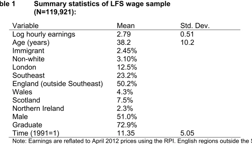
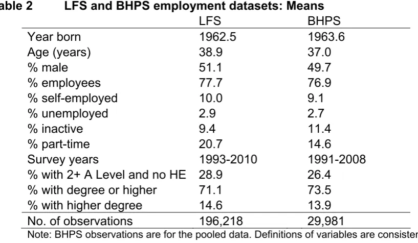
The dependent variable is based on the LFS-derived variable "hourpay", which is defined as the ratio of usual earnings to usual hours (from main job) including paid overtime. For pre-1996 LFS, where this derived variable is not available, we compute the variable using the same formula using the same raw data. Similar results hold using the reported hourly wage rate in the data. However, only a small proportion of graduates report an hourly wage rate. From 1997Q3 onwards, LFS also collects wage information in W1 (as well as W5). This allows us to construct a short wage-panel to be used in the first step of the two-step estimation to provide estimates of the lifecycle of earnings. Table 1 gives brief summary statistics.

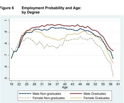
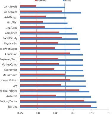
Figure 4 shows the distribution of log real hourly earnings by sex and graduate status in the raw LFS data. Rather than present a histogram, which would have a jagged shape, we “smooth” the raw data to yield what is known as a kernel density plot. The solid lines show the distributions of graduate earnings, while the dotted lines show the distributions for non-graduates. There is clearly higher variance and lower mean amongst non-non-graduates. Figure 5 shows how log hourly earnings vary with age. There is clearly a strong age pattern in earnings and the differential between graduates and non-graduates is smaller earlier in the lifecycle. Figure 6 shows how the employment probability varies with age. Here the differences by graduate status seem broadly similar across age. Graduate

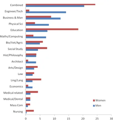
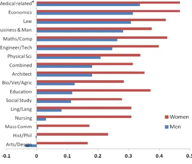
employment is higher than non-graduate across all ages. Of course, these graphs conceal cohort effects as well as true lifecycle effects. Figure 7 shows the distribution of the data across degree subject studied.