Value-Gradient Learning

      

City, University of London Institutional Repository

Citation

:

Fairbank, M. and Alonso, E. (2012). Value-Gradient Learning. Paper presented

at the WCCI 2012 IEEE World Congress on Computational Intelligence, 10-06-2012 -

15-06-2012, Brisbane, Australia.

This is the accepted version of the paper.

This version of the publication may differ from the final published

version.

Permanent repository link: http://openaccess.city.ac.uk/5205/

Link to published version

:

http://dx.doi.org/10.1109/IJCNN.2012.6252791

Copyright and reuse:

City Research Online aims to make research

outputs of City, University of London available to a wider audience.

Copyright and Moral Rights remain with the author(s) and/or copyright

holders. URLs from City Research Online may be freely distributed and

linked to.

Value-Gradient Learning

Michael Fairbank

Department of Computing, School of Informatics, City University London,

London, UK

Email: [email protected]

Eduardo Alonso

Department of Computing, School of Informatics, City University London,

London, UK Email: [email protected]

Abstract—We describe an Adaptive Dynamic Programming algorithm VGL(λ) for learning a critic function over a large continuous state space. The algorithm, which requires a learned model of the environment, extends Dual Heuristic Dynamic Programming to include a bootstrapping parameter analogous to that used in the reinforcement learning algorithm TD(λ). We provide on-line and batch mode implementations of the algorithm, and summarise the theoretical relationships and motivations of using this method over its precursor algorithms Dual Heuristic Dynamic Programming and TD(λ). Experiments for control problems using a neural network and greedy policy are provided.

Index Terms—Value-Gradient Learning, Dual Heuristic Dy-namic Programming, DHP, Adaptive DyDy-namic Programming

I. INTRODUCTION

Adaptive Dynamic Programming (ADP, [1]) is the study of how an agent can learn to choose actions that minimise a total long-term cost. For example a typical scenario is an agent wandering around in an state space S ⊂ <n, such that

at time t it has state vector~xt∈S. At each timet the agent

chooses an action ~ut (from an action space ~ut ∈ A) which

takes it to the next state according to the environment’s model function ~xt+1 = f(~xt, ~ut), and gives it an immediate scalar

costUt, given by the functionUt=U(~xt, ~ut). The agent keeps

moving, forming a trajectory of states (~x0, ~x1, . . .), which

terminates if and when a state from the set of terminal states

T ⊂ S is reached. If a terminal state ~xt ∈ T is reached

then a final instantaneous cost Ut = U(~xt) is given which

is independent of any action.

Anaction networkoractororpolicy function,A(~x, ~z), is a neural network (or more generally, a function approximator) with parameter vector ~z, which specifies which action ~u =

A(~x, ~z)to take for any given state~x. From any given state~x, the expectation of the total future long term cost encountered when following actions chosen by an action networkA(~x, ~z), is given by the function J(~x, ~z) = hP

tγ t_U

ti, where hi

denotes expectation. This is the cost-to-go function for the given action network, also known as the value functionfrom dynamic programming [2] and reinforcement learning (RL, [3]). Hereγ∈[0,1]is a constantdiscount factorthat specifies the importance of long term costs over short term ones. The objective of ADP and RL is to train the action network to choose actions that minimise the total cost-to-go function from any state~x.

ADP also uses a second neural network (or function ap-proximator), Je(~x, ~w) ∈ <, with weight vector w~, known as

the critic or approximate value function. The intermediate objective of ADP is to train the critic to approximate the cost-to-go function, so thatJe(~x, ~w)≈J(~x, ~z)for all~x∈_S. If this

is achieved perfectly, and ifsimultaneouslythe action network always chooses actions according to:

~

u= arg min ~ u∈A

D

U(~x, ~u) +γJe(f(~x, ~u), ~w) E

∀~x (1) then Bellman’s Optimality Condition [2] shows the trajectories produced will be optimal, and the action network is optimal.

The method of choosing actions purely by equation 1 is called thegreedy policy onJesince it chooses actions that the

critic rates as best.

The ADP method Heuristic Dual Programming (HDP), and the RL methods TD(λ) and Q-learning [4], [5], are all critic learning methods that sample trajectories and update the critic values encountered along the trajectory. We call these methods

value learning(VL) methods since they learn the values ofJe

along the trajectory. Variants of these methods have produced successes in control problems [6], [7], but they can be very slow since Bellman’s condition needs meeting over the entire continuous state space for optimality. Even if Bellman’s condi-tion is perfectly satisfied along a single trajectory, performance can be extremely far from optimal. Bellman’s condition must be satisfied at least on the neighbouring trajectories too for local optimality. Hence VL methods must be supplemented by exploration of the environment just to attain local optimal-ity. This exploration could be provided by stochastic model functions, a stochastic policy, or a stochastic start point for each trajectory. The methods we follow significantly reduce the need for this explicit exploration.

optimality, VGL methods only need learn the value-gradient along the single trajectory to achieve the same assurance of local optimality. This motivation is discussed further in section I-A. Also, VGL methods can work very well in control problems in continuous state spaces.

We extend the VGL methods from DHP to include a bootstrapping parameter λ ∈ [0,1] (just as TD(λ) is an extension of TD(0)), to give the algorithm we call VGL(λ), which we describe in this paper. For λ = 0, VGL(λ) is equivalent to DHP, but forλ >0, VGL(λ) is a new algorithm. The motivations for this extension are that using λ > 0

can increase the stability of learning and sometimes increase learning speed, as discussed further in section I-B.

VGL methods (including DHP) are model-based methods that require a learned differentiable model of the environment and cost functions,f(~x, ~u)andU(~x, ~u). We discuss this more in section I-C.

In sections I-A and I-B, we expand on the motivations for VGL methods and the λ parameter, and in section I-C we discuss the applicability of VGL methods and the necessary learning of the model functions. In the rest of the paper, we define the VGL(λ) algorithm in section II, and state its relationship to TD(λ) and DHP in subsections II-C and II-D. In section III, we give experimental results, and finally, in section IV we give conclusions.

A. Motivations for DHP and VGL Methods

The VGL (and hence DHP) methods address the issue of the Bellman equation needing to be solved over the whole of state space, in that it turns out to be only necessary to fully learn the value gradient along a single trajectory, under a greedy policy, for it to be locally extremal, and often locally optimal. This is proven by [11], and is closely related to Pontryagin’s Minimum Principle [12]. This optimality condition contrasts strongly with the VL methods which need to learn the value function over all immediately neighbouring trajectories too in order to achieve the same level of guarantee for being locally extremal/optimal trajectories. So this is a significant efficiency gain for the VGL methods, and is their principal motivation.

This implies that VGL methods have a much lesser require-ment for exploration than VL methods do, since the local

part of exploration comes for free by using VGL methods. What we mean by this is that provided the VGL learning algorithm makes progress in learning the value gradient all along a trajectory, while following a greedy policy, then the trajectory will automatically make progress in bending itself towards a locally optimal shape. This will happen without the need for any stochastic exploration. In effect, by using VGL methods, local exploration is automatic; or put another way the traditional RL dilemma of “exploration versus exploitation” transforms into “explorationandexploitation”, locally at least. This leads to greater efficiency for VGL compared to VL. In comparison the failure of VL without any exploration in a deterministic environment is dramatic and common, even when the value-function is perfectly learned along a single trajectory. The experiment in section III-A confirms this.

Both VL and VGL methods have the same requirement for global optimality, that is if the value function (or its gradient) is exactly learned over all of state space, with a greedy policy, then Bellman’s condition assures global optimality.

For a fuller discussion of the motivations to use VGL methods see [13].

B. Motivations for Introducing theλParameter into DHP

The motivations for using theλparameter are that choosing

λcarefully can increase the stability of learning and sometimes increase learning speed.

For example, when λ = 1, the weight update used by TD(λ) for a fixed action network is true gradient descent on an error function and so is guaranteed to converge [4]. However when λ = 0, TD(λ) is not true gradient descent on any error function, and this weight update can diverge when the approximator for Je(~x, ~w) is non-linear inw~ [14].

Similarly, DHP is not true gradient descent on any function, and general instability in this case has been proven [15, sec. 7.7-7.8]. However VGL(1) is true gradient descent on an error function, for a fixed action network, and so will converge.

Furthermore, when a greedy policy is used, all of TD(1), TD(0) and DHP can be made to diverge [16]. However with carefully chosen learning parameters and smoothness assumptions, VGL(1) can be guaranteed to converge with a greedy policy, as discussed further in section II. In this case VGL(1) becomes identical to backpropagation through time [17] acting directly on the greedy policy, as proven by [11].

Choosingλcarefully can affect the learning speed of critic learning algorithms. Having a high value of λ makes the target in the critic weight update use a longer “look-ahead” along the trajectory, and so this can improve learning speed. However, conversely, having too large a value ofλcan increase the variance of the sampled target J value in a stochastic environment, which can slow down learning. Hence in TD(λ), often the optimal value ofλfor learning speed is somewhere in the middle range ofλ∈[0,1], as demonstrated by [3].

C. Applicability of VGL methods and System Identification

The VGL methods are strictly model-based methods, and this is largely where the extra efficiency comes from. We assume the model functions can be learned by a separate “sys-tem identification” learning process, for example as described by [18]. This system identification process could have taken place prior to the main learning process (e.g. like [19]), or concurrently with it, and results in learned model functions

f(~x, ~u)andU(~x, ~u). Alternatively, there is an extremely fast on-line model-learning method by [20] which could be used. We do not describe this model-learning stage of the process any further in this paper.

DHP successes include autopilot landing [10], power system control [21] and many others [1]. However some traditional RL problem domains with discrete spaces would not be readily solvable by VGL methods, such as a “grid world” problem, backgammon, or a k-armed bandit problem. Also, step cost functions would not be applicable, thus excluding problems such balancing a pole where the total cost is a function of theintegernumber of time steps that the pole is balanced for. However the pole balancing problem can be solved by DHP if a smoothed out cost function is used [22]. As a rule of thumb, if a problem is suitable for smooth gradient descent onJ with respect tow~, then it will be suitable to work on VGL methods.

II. THEVGL(λ) ALGORITHM

In this section we define the VGL(λ) Algorithm and state how it relates to the algorithms TD(λ) and Dual Heuristic Dynamic Programming.

To define the VGL(λ) algorithm, we require that Je(~x, ~w)

is defined by a smooth scalar function approximator, e.g. a neural network with weight vector w~. This enables us to define the “critic gradient”, or “approximate value gradient”, as Ge(~x, ~w)≡

∂Je(~x, ~w)

∂~x .

Throughout this paper, a convention is used that all defined vector quantities are columns, whether they are coordinates, or derivatives with respect to coordinates. So, for example,Ge

and ∂Je

∂~x are columns. Also, all subscripted indices are what we

calltrajectory shorthand notation. These refer to the time step of a trajectory and provide corresponding arguments ~xt and

~

utwhere appropriate; so that for exampleJet+1≡Je(~xt+1, ~w)

andGet≡Ge(~xt, ~w).

Differentiating a column vector function by a column vector causes the vector in the numerator to become transposed (becoming a row).1 _{For example} ∂f

∂~x is a matrix with element (i, j)equal to∂f(_∂~~x,~_xiu)j. Similarly,

∂Ge

∂ ~w

ij

=∂Gej

∂ ~wi, and

∂Ge

∂ ~w

t

is this matrix evaluated at(~xt, ~w).

Then, using this notation and the implied matrix products, the VGL(λ) algorithm can be defined as a weight update of the form:

∆w~ =αX

t

∂Ge

∂ ~w

!

t

Ωt(G0t−Get) (2)

whereαis a small positive learning rate;Getis the critic

gradi-ent; and G0t is the “target value gradient” defined recursively

by:

G0t=

DU D~x t +γ Df D~x t

λG0t+1+ (1−λ)Get+1

(3)

withG0t= ∂U_∂~x

tat any terminal state; whereλ∈[0,1]is a

constant; where Ωt is an arbitrary positive definite matrix of dimension (dim~x×dim~x); and where _D~D_x is shorthand for

D D~x ≡

∂ ∂~x+

∂A ∂~x

∂

∂~u ; (4)

1_{This is the opposite of a common convention.}

and where all of these derivatives are assumed to exist. We ensure the recursion in eq. 3 converges by requiring that either γλ < 1, or the environment is such that the agent is guaranteed to reach a terminal state at some finite time (i.e. the environment is “episodic”). Equations 2, 3 and 4 define the VGL(λ) algorithm. Section II-B gives further implementation details and pseudocode.

The target value-gradients, G0, are so called because the VGL objective is to achieve Get = G0t for all t along a

trajectory. This objective ensures a locally extremal, and often locally optimal, trajectory (as proven by [11]), when combined with a greedy policy. It should be noted that this objective is not straightforward to achieve since the targetsG0tare moving

ones and are highly dependent onw~ (especially when a greedy policy is being used, so that then the policy is alsoindirectly

dependent on w~). Hence we must use the weight update to

slowlymove the approximated gradients towards their targets. TheΩtmatrix was introduced by Werbos for the algorithm GDHP (e.g. see [15, eq. 32]), which is very closely related to VGL(λ). It is a free parameter, included for generality, since the presence of any positive definite matrix here in equation 2 will force every component of Get to move towards the

corresponding component of G0t (in any basis). It is often

just taken to be the identity matrix for simplicity. However for the special choice of

Ωt=    _∂f ∂~u T

t−1

_∂2

e

Q ∂~u∂~u

−1

t−1

_∂f

∂~u

t−1 for t >0

0 for t= 0

, (5) the algorithm VGL(1) is proven to converge for a sufficiently small learning rate and when used in conjunction with a greedy policy, under certain smoothness assumptions [11]. HereQe is

the approximate Q Value function defined by

e

Q(~x, ~u, ~w) =U(~x, ~u) +γJe(f(~x, ~u), ~w). (6) A. Action Network Training Algorithm and Greedy Policy

The VGL(λ) algorithm is for training a critic function. To make the agent learn to behave optimally, the action network function A(~x, ~z) also needs training. We follow the method of [10], which uses the following weight update for the action network at each time stept:

∆~z=−β

∂A ∂~z t ∂U ∂~u t +γ ∂f ∂~u t e

Gt+1

(7) where β is a separate learning rate for the action network. The multiplication by ∂A_∂~z can be done quickly and exactly by ordinary backpropagation. This weight update can be done concurrently with the critic weight update, or by iteratively doing several critic weight updates followed by several action network weight updates.

The above weight update is equivalent to ∆~z = −β ∂A_∂~z

t _∂ e Q ∂~u t

, which is direct gradient descent on the function Qe(~xt, A(~xt, ~z), ~w) with respect to ~z, where Qe is

A(~x, ~z) = arg min ~

u∈A(Qe(~x, ~u, ~w)) ∀~x. (8)

In some circumstances we can omit the action network altogether and just use the right hand side of equation 8 directly, forming the greedy policy (as in equation 1). This saves the difficulty of having to simultaneously train the critic and action networks, which may interfere with each other in unpredictable ways. Instead it makes the action network appear to be always fully trained. A greedy policy is only possible when the right hand side of equation 8 is efficient to compute, which is common in the continuous time situations described by [7] or [23, section 2.2]. In this case the greedy policy often reduces to

(~ut)i≡g

−

_∂U

∂~ui

t −γ

_∂f

∂~ui

t

e

Gt

, (9) where g(x) is a chosen sigmoid function, for example a hyperbolic tangent or logistic function. This greedy policy equation produces actions that are bound to the range of

g(x), and it is conveniently efficient and differentiable, so is applicable for use in the VGL(λ) algorithm. We give an example of this kind of greedy policy in section III-C.

B. Implementation of VGL(λ)

We now give pseudocode for two different ways of imple-menting the VGL(λ) algorithm - one is for on-line learning which can be continually applied as trajectories are expanded, and one is a batch mode implementation which is slightly more efficient but is only applicable to completed trajectories.

When implementing VGL(λ), the functionGe(~x, ~w)can be

implemented in two different possible ways. Since Ge(~x, ~w)

is defined to be ∂Je(~x, ~w)

∂~x , the appearance of the term ∂Ge

∂ ~w in

equation 2 is defined to mean ∂2Je

∂ ~w∂~x. We refer to this method of

implementation as using ascalar critic function,Je(~x, ~w), or a GDHP style critic. However an alternative, easier, method is to implement Ge(~x, ~w)directly as the output of a smooth vector

function approximator of output dimension dim(~x). In this case the scalar function Je(~x, ~w) is never actually needed in

VGL(λ). We refer to this alternative method of implementation as using a vector criticfunction,Ge(~x, ~w), or as using aDHP style critic. Either of these two approaches is a valid way to implement the VGL(λ) algorithm.

Algorithm 1 makes a direct implementation of VGL(λ) for episodic environments. It makes a forward pass through the trajectory, storing all states and actions, followed by a backward pass through the trajectory accumulatingG0

tby the

recursion in Eq. 3.

In this implementation, if a neural network is used to output the function Ge(~x, ~w), then the matrix-vector products

involving ∂Ge

∂ ~w can be calculated in time O(dim(w~)), by using

backpropagation. Similarly, if Ge ≡ _{∂ ~}∂_wJe, where Je is the

scalar output of a neural network, then the matrix product involving second order derivatives ∂Ge

∂ ~w can still be evaluated

in the same time, by using methods analogous to those of

Algorithm 1 VGL(λ). Batch-mode implementation for episodic environments.

1: t←0

2: {Unroll trajectory...}

3: while not terminated(~xt)do

4: ~ut←A(~xt, ~z)

5: ~xt+1←f(~xt, ~ut)

6: t←t+ 1

7: end while

8: F ←t

9: ~p← ∂U ∂~x

t,∆w~ ←~0,∆~z←~0

10: {Backwards pass...}

11: fort=F−1to0 step−1do

12: G0t← ∂U_∂~x

t+γ

∂f ∂~x

t

~ p

+ ∂A_∂~x

t

∂U ∂~u

t+γ

_∂f

∂~u

t

~ p

13: ∆w~ ←∆w~ +∂Ge

∂ ~w

tΩt

G0t−Get

14: ∆~z←∆~z− ∂A_∂~zt

∂U ∂~u

t+γ

∂f ∂~u

t

e

Gt+1

15: ~p←λG0t+ (1−λ)Get

16: end for

17: w~ ←w~+α∆w~

18: ~z←~z+β∆~z

[24]. The matrix products involving ∂A_∂~x can also be evaluated quickly using backpropagation. Hence the whole algorithm takes O(n) operations per time step of the trajectory, where

n= max(dim(w~),dim(~z)).

For nepisodic environments, Algorithm 2 gives an on-line implementation of VGL(λ). Unlike the previous algo-rithm, this one does not require that the trajectory reaches a terminal state before the weight update can be applied. This algorithm runs in a slower time of O(dim(w~) dim(~x)2₎

operations per time step of the trajectory, and its derivation is given by [11, Appendix B]. In the case of λ = 0, the algorithm can be optimised to remove the variable E, and then the algorithmic complexity drops to be the same as that of Algorithm 1.

Neither algorithm attempts to learn the value gradient at the final time-step of a trajectory since it is prior knowledge that the target value gradient is always ∂U_∂~x at any terminal state. Hence we assume the function approximator forGe(~x, ~w)has

been designed to explicitly return ∂U_∂~x for all terminal states~x. Both algorithms incorporate the action network weight update of equation 7. If a different actor weight update scheme was needed then these lines could be moved or replaced, and similarly if a greedy policy was used then these lines would be removed.

C. Relationship to TD(λ)

Algorithm 2 VGL(λ). On-line implementation.

1: E ← 0 {E ∈ <dim(w~)×dim(~x) is an “eligibility trace” workspace matrix.}

2: t←0

3: whilenot terminated(~xt)do

4: ~ut←A(~xt, ~z)

5: ~xt+1←f(~xt, ~ut)

6: ~δ← ∂U_∂~xt+ ∂A_∂~xt ∂U_∂~ut

+γ∂f_∂~x

t + ∂A

∂~x

t

_∂f

∂~u

t

e

Gt+1−Get

7: E←E+∂Ge

∂ ~w

t Ωt

8: w~ ←w~+αE~δ

9: E←λγE∂f_∂~x

t+ ∂A ∂~x

t

_∂f

∂~u

t

10: ~z←~z−β ∂A_∂~zt

∂U ∂~u

t+γ

∂f ∂~u

t

e

Gt+1

11: t←t+ 1 12: end while

learned by a neural network. Hence the VGL(λ) algorithm has a very similar form to that of TD(λ).

For a given trajectory, the following critic weight update is equivalent to the TD(λ) algorithm:

∆w~ =αX

t

∂Je

∂ ~w

!

t

(J0t−Jet) (10)

whereJ0 is defined recursively by

J0t=Ut+γ

λJ0t+1+ (1−λ)Jet+1

(11) with J0t=Ut at any terminal state, and where λ∈[0,1]is

a fixed global constant. For convergence of this recursion we require that either γλ < 1, or the environment is episodic, just like the recursion in equation 3. To understand the equivalence of this weight update to the TD(λ) algorithm originally described by [4], first we note that J0 as defined by equation 11 is identical to the “λ-return” of [5], as proven by [11, Appendix A]. Hence equation 10 is an application of what [3] describe as the “forwards view of TD(λ)”, and hence is equivalent to the TD(λ) weight update (see [11, Appendix A] for further details).

Since J0t is defined for an arbitrary trajectory, we can

rewrite its recursive definition as

J0(~xt, ~w, ~z) =U(~xt, A(~xt, ~z)) +γ(λJ0(f(~xt, A(~xt, ~z)), ~w) +(1−λ)Je(f(~xt, A(~xt, ~z)), ~w)

(12) We can now obtain the relationship of VGL(λ) to TD(λ). Differentiating equation 12 fully with respect to ~xt (and

applying the chain rule, ~ut = A(~xt, ~z), ~xt+1 = f(~xt, ~ut),

e

G ≡ ∂Je

∂~x and trajectory shorthand notation) produces the

same recursion as equation 3. This proves that G0 ≡ ∂J0 ∂~x.

Furthermore, replacing all of the termsJeandJ0in the TD(λ)

weight update by their derivatives with respect to~xproduces the VGL(λ) weight update (with Ωt ≡ I). Hence VGL(λ) is a differentiated form of TD(λ); whereas TD(λ) attempts

to learn values, VGL(λ) attempts to learn value gradients. The reason VGL(λ) does this is because value-gradients are what the greedy policy uses to decide which actions to take (for example see equation 9, or see section I-A for a further discussion).

D. Relationship to Dual Heuristic Dynamic Programming

The algorithm Dual Heuristic Dynamic Programming (DHP) by [8] and described more recently by [10], [1] is identical to VGL(0) with a vector critic. The DHP algorithm has been designed with similar motivations as ours, and pre-dates our work. Our implementation VGL(λ) generalises it to include a bootstrapping parameterλanalogous to that used in TD(λ). The relationship of DHP to VGL(λ) is identical to the relationship of TD(0) to TD(λ).

The algorithm Globalized Dual Heuristic Dynamic Pro-gramming (GDHP) is identical to a weight update that is a linear combination of VGL(0) with a scalar critic and TD(0).

III. EMPIRICAL RESULTS

We describe neural network experiments for two control problems: a simple quadratic optimisation problem and a verti-cally moving spacecraft simulation. We show the performance of VL versus VGL methods, and also investigate the effects of varying the λparameter andΩt matrix.

A. Quadratic Optimisation Problem

We now describe a quadratic optimisation experiment using an actor-critic architecture, and compare the effectiveness of VGL(λ) to TD(λ) in the situation of both noisy and deter-ministic policies. This shows the motivation for VGL based methods in that they work very quickly and that they can do local exploration even while only following deterministic trajectories.

We define an environment with~x=x∈ <and~u=u∈ <, and model and cost functions:

f(x, t, u) =x+u U(x, t, u) = (u)2

Each trajectory is defined to terminate on arriving at time step t = 2, and on termination a final instantaneous cost of

U(~x) = (x)2 is given. The only actions used in the trajectory are u0 and u1; the total cost for this trajectory is (u0)2+

(u1)2+ (x0+u0+u1)2, and the theoreticaloptimaltotal cost

for the whole trajectory is J∗= (x0)2/3.

The action network was a multi-layer perceptron (MLP, see [26] for details) with two inputs, one output and one hidden layer of 4 nodes, shortcut connections from the input layer to the output layer, and with activation functiong(x) = tanh(x)

at all nodes. The weights ~z were initially randomised uni-formly from the range [-0.1, 0.1]. The critic networkJe(~x, ~w)

node, which used g(x) =x. The input vector to each neural network was (x, t).

Each trajectory was made to start at x0 = 0.8. Learning

rates for the critic and actor were both α= 0.1 andβ= 0.1, respectively, with discount factorγ= 1. To provide the facility for exploration, Gaussian noise with mean zero and variance

σ2was added to the output of the action network to form the policy function, A(~x, ~z).

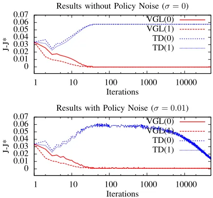
The critic learning algorithms tested were TD(1), TD(0), VGL(1) and VGL(0). The action network’s weight update was done by equation 7 in all experiments. We repeated the experiments with noise (σ= 0.01) and without noise (σ= 0). Results averaged from 40 trials for each algorithm are shown in figure 1. The results show that the value-learning method (TD(λ)) could not cope without some random exploration, but the VGL based methods (GDHP and VGL(λ)) work successfully for both σ values used. Also, in comparison to the value learning methods, VGL methods are very fast. On the other-hand VGL methods require knowledge of the model functions (in order to use their derivatives), whereas VL methods do not. But when the model functionsare available, the increased speed and automatic local exploration provides a strong motivation to use VGL methods.

0 0.01 0.02 0.03 0.04 0.05 0.06 0.07

1 10 100 1000 10000

J-J*

Iterations

Results without Policy Noise (σ= 0) VGL(0) VGL(1) TD(0) TD(1)

0 0.01 0.02 0.03 0.04 0.05 0.06 0.07

1 10 100 1000 10000

J-J*

Iterations

[image:7.612.52.270.339.542.2]

Results with Policy Noise (σ= 0.01) VGL(0) VGL(1) TD(0) TD(1)

Fig. 1. Algorithm performances for the quadratic optimisation problem of section III-A, both with and without policy noise. Theyaxis showsJ−J∗_,

whereJ∗is the optimal trajectory cost. Compared to the VL method (TD(λ)), the VGL method works well in the absence of stochastic exploration, and quickly attainsJ=J∗. The VL method fails without stochastic exploration here (i.e. it converges to a suboptimal policy), but does learn slowly and successfully in the presence of policy noise.

B. Vertical Spacecraft Problem

In this section we consider a neural network controlled spacecraft.

A spacecraft of mass m is dropped in a uniform gravita-tional field. The spacecraft is constrained to move in a vertical line, and a single thruster is available to make upward acceler-ations. The state vector of the spacecraft is~x= (h, v, t)T _and

has three components: height (h), velocity (v) and time step (t). The action vector is one-dimensional (so that~u≡u∈ <) producing accelerations u ∈ [0,1]. The Euler method with time-step∆tis used to integrate the equation of motion, giving the model function:

f((h, v, t)T, u) =(h+v∆t, v+ (u−kg)∆t, t+ 1)T

Here,kg= 0.2 is a constant giving the acceleration due to

gravity (which is less than the range of u; so the spacecraft can overcome gravity easily).∆t was chosen to be 0.4.

A trajectory is defined to last exactly 200 time steps. A final impulse of cost equal to

U(~x) =1 2mv

2_+m(k

g)h (14)

is given on completion of the trajectory. This cost penalises the total kinetic and potential energy that the spacecraft has at the end of the trajectory. This means the task is for the spacecraft to lose as much mechanical energy as possible throughout the duration of the trajectory, to prepare for a gentle landing. The optimal strategy for this task is to leave the thruster switched off for as long as possible in the early stages of the journey, so as to gain as much downward speed as possible and hence lose as much potential energy as possible, and at the end of the journey produce a burst of continuous maximum thrust to reduce the kinetic energy as much as possible.

In addition to the cost received at termination by equation 14, a cost is also given for each non-terminal step. This cost is

U(~x, u) =c

₁

2ln(2−2u)−uarctanh(1−2u)

∆t (15) wherec= 0.02 is constant. This cost function is designed to ensure that the actions chosen will satisfy u∈[0,1], even if a greedy policy is used. We explain how this cost function was derived, and how it can be used in a greedy policy, in section III-C, but first we describe experiments that did not use a greedy policy.

A DHP-style critic, Ge(~x, ~w), was provided by a fully

connected MLP with 3 input units, two hidden layers of 6 units each, and 3 units in the output layer. Additional short-cut connections were present fully connecting all pairs of layers. The weights were initially randomised uniformly in the range [−.1, .1]. The activation functions were logis-tic sigmoid functions in the hidden layers, and the identity function in the output layer. The input to the MLP was

(h/1600, v/40, t/200)T and the output gave Ge directly.

The action network was identical in design to the critic, except there was only one output node, and this had a logistic sigmoid function as its activation function. The output of the action network gave the spacecraft’s accelerationudirectly.

Results using the actor-critic architecture and Algorithm 1 are given in figure 2 comparing the performance of VGL(1) and VGL(0) (DHP). Each curve shows algorithm performance averaged over 40 trials.

The graphs show that the VGL(1) algorithm produces a lower total costJ than the VGL(0) algorithm does, and does it faster. It is thought that this is because in this problem the major part of the total cost comes as a final impulse, so it is advantageous to have a long look-ahead (i.e. a high λvalue) for fast and stable learning.

For the actor-critic learning we chose the learning rate of the actor to be high compared to the learning rate for the critic (i.e.β > α). This was to make the results comparable to those of a greedy policy which we try in the next section.

0 5 10 15 20

1 10 100 1000 10000 100000

J

Iterations

VGL(0) and VGL(1) using Actor-Critic

[image:8.612.323.533.206.301.2]

VGL(0) VGL(1)

Fig. 2. VGL(0) (i.e. DHP) and VGL(1), with Actor-Critic, using learning ratesα= 10−6_{andβ= 0.01.}

C. Vertical Spacecraft Problem with Greedy Policy

The cost function of equation 15 was derived to form an efficient greedy policy, by following the method of [7]. First we chose the sigmoid function g(x) that we would like the greedy policy of equation 9 to use. This was chosen to be

g(x) =1

2(tanh(x/c) + 1).

The choice ofcaffects the sharpness of this sigmoid function. Using this chosen sigmoid function, the cost function based on [7] is defined to be

U(~x, u) = ∆t

Z

g−1(u)du. (16) Note that solving this integral gives equation 15. Then to derive the greedy policy for this cost function, we make a first order Taylor series expansion of the Qe(~x, ~u, ~w)function

(eq. 6) about the point ~x:

e

Q(~x, ~u, ~w)≈U(~x, ~u) +γ

 

∂Je

∂~x

!T

(f(~x, ~u)−x~) +Je(~x, ~w)  

=U(~x, ~u) +γGe(~x, ~w) T

(f(~x, ~u)−x~) +γJe(~x, ~w)

(17) This approximation becomes exact in continuous time, i.e. in the limit as ∆t → 0. The greedy policy must minimise Qe,

hence we differentiate equation 17 to get

∂Qe

∂u

!

t =

_∂U

∂u

t +γ

_∂f

∂u

t

e

Gt by eq. 17

=g−1(ut)∆t+γ

_∂f

∂u

t

e

Gt by eq. 16

For a minimum, we must have ∂Qe

∂u = 0, which, since ∂f ∂u is

independent of u, gives ut = g

−_∆γ_t∂f_∂u tGet

. This is a variation on equation 9, and we used it as the greedy policy for the experiments in Figure 3. The results show similarrelative

performance of VGL(1) versus VGL(0) as in the actor-critic experiments, and both algorithms are faster than when an actor was used. This indicates that in this experiment, the greedy policy derived can successfully replace the action network, raising efficiency, and without any apparent detriment.

0 5 10 15 20

1 10 100 1000 10000

J

Iterations

VGL(0) and VGL(1) using a Greedy Policy

VGL(0) VGL(1)

Fig. 3. VGL(0) (i.e. DHP) and VGL(1), with a greedy policy, using a learning rateα= 10−6.

0 5 10 15 20

0 200 400 600 800 1000 1200 1400

J

Iterations

VGL(0) using RPROP and a Greedy Policy

0 5 10 15 20

0 200 400 600 800 1000 1200 1400

J

Iterations

VGL(1) using RPROP and a Greedy Policy

0 5 10 15 20

0 200 400 600 800 1000 1200 1400

J

Iterations

VGLΩ(1) using RPROP and a Greedy Policy

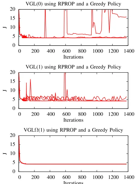
Fig. 4. VGL(0), VGL(1) and VGLΩ(1), with a greedy policy, using RPROP. Each graph shows the performance of a learning algorithm for each of five different weight initialisations; hence the ensemble of curves in each graph gives some idea of an algorithm’s reliability and volatility.

[image:8.612.60.271.230.325.2] [image:8.612.319.544.348.653.2]

interacting neural networks whose training could be interfering with each other. With the simpler architecture of just one neural network (the critic) to contend with, we attempt to speed up learning using RPROP [27]. Results as shown in figure 4. It seems the aggressive acceleration by RPROP can cause large instability in the VGL(1) and DHP algorithms. This is because neither of these two algorithms is true gradient descent when used with a greedy policy [16]. However when theΩtmatrix defined by equation 5 is used withλ= 1, giving the algorithm that we will refer to as VGLΩ(1), the resulting algorithm is true gradient descent. It is gradient descent on

J, as proven by [11]. The performance of this algorithm is shown in the bottom graph of Figure 4, and this shows the minimum being reached stably and many times quicker than in the actor-critic or non-RPROP case.

This represents a significant breakthrough in making learn-ing with a greedy policy exhibit reliable and monotonic progress. The Ωt equation that achieves this is only proven

to work for VGL(1), and counterexamples exist for its use with DHP [16].

IV. CONCLUSIONS

We have defined the VGL(λ) algorithm and explained its relationship to its precursor algorithms DHP and TD(λ). VGL(λ) can be viewed as a differentiated form of TD(λ); whereas TD methods learn values, VGL methods learn value-gradients. VGL(λ) extends the DHP algorithm by introducing a bootstrapping parameter, λ, which can affect learning speed and stability.

We have described the motivations for using VGL based methods (including DHP) in comparison to VL methods. These are that local exploration is automatic; VGL methods can be many times faster than VL methods; and VGL methods work naturally in continuous state spaces. The experiments confirmed these motivations, showing success for VGL in environments when no exploration is used and where VL methods fail. The experiments also demonstrate that VGL methods can be many times faster than VL methods. However, unlike VL methods, VGL methods require that the model functions are differentiable, and known or learnable.

Learning value-gradients is theoretically motivated since value-gradients can drive a greedy policy (e.g. as in equation 9), and the greedy policy equation (in the form of equation 1) must be satisfied if Bellman’s Optimality Principle is to apply; so explicitly learning value-gradients is a very direct way to achieve optimal trajectories, without the need for local exploration.

The experiments demonstrated that when the special Ωt

matrix of equation 5 is used, then the VGLΩ(1) algorithm can produce very stable learning with a greedy policy. This is a proven convergent critic learning algorithm, under certain smoothness assumptions, with a general function approximator and a greedy policy.

REFERENCES

[1] F.-Y. Wang, H. Zhang, and D. Liu, “Adaptive dynamic programming: An introduction,” IEEE Computational Intelligence Magazine, vol. 4, no. 2, pp. 39–47, 2009.

[2] R. E. Bellman,Dynamic Programming. Princeton, NJ, USA: Princeton University Press, 1957.

[3] R. S. Sutton and A. G. Barto,Reinforcement Learning: An Introduction. Cambridge, Massachussetts, USA: The MIT Press, 1998.

[4] R. S. Sutton, “Learning to predict by the methods of temporal differ-ences,”Machine Learning, vol. 3, pp. 9–44, 1988.

[5] C. J. C. H. Watkins, “Learning from delayed rewards,” Ph.D. disserta-tion, Cambridge University, 1989.

[6] C. Kwok and D. Fox, “Reinforcement learning for sensing strategies,” in Proceedings of the International Confrerence on Intelligent Robots and Systems (IROS), 2004.

[7] K. Doya, “Reinforcement learning in continuous time and space,”Neural Computation, vol. 12, no. 1, pp. 219–245, 2000.

[8] P. J. Werbos, “Approximating dynamic programming for real-time control and neural modeling.” inHandbook of Intelligent Control, D. A. White and D. A. Sofge, Eds. New York: Van Nostrand Reinhold, 1992, ch. 13, pp. 493–525.

[9] S. Ferrari and R. F. Stengel, “Model-based adaptive critic designs,” in

Handbook of learning and approximate dynamic programming, J. Si, A. Barto, W. Powell, and D. Wunsch, Eds. New York: Wiley-IEEE Press, 2004, pp. 65–96.

[10] D. Prokhorov and D. Wunsch, “Adaptive critic designs,”IEEE Transac-tions on Neural Networks, vol. 8, no. 5, pp. 997–1007, 1997. [11] M. Fairbank and E. Alonso, “The local optimality of reinforcement

learning by value gradients, and its relationship to policy gradient learning,” CoRR, vol. abs/1101.0428, 2011. [Online]. Available: http://arxiv.org/abs/1101.0428

[12] L. S. Pontryagin, V. G. Boltayanskii, R. V. Gamkrelidze, and E. F. Mishchenko, The Mathematical Theory of Optimal Processes (Trans-lated from Russian). Wiley, 1962, vol. 4.

[13] M. Fairbank and E. Alonso, “A comparison of learning speed and ability to cope without exploration between DHP and TD(0),” inProceedings of the IEEE International Joint Conference on Neural Networks 2012 (IJCNN’12). IEEE Press, June 2012, pp. 1478–1485.

[14] J. N. Tsitsiklis and B. Van Roy, “An analysis of temporal-difference learning with function approximation,” IEEE Transactions on Automatic Control, Tech. Rep., 1996.

[15] P. J. Werbos, “Stable adaptive control using new critic designs,”eprint arXiv:adap-org/9810001, 1998.

[16] M. Fairbank and E. Alonso, “The divergence of reinforcement learning algorithms with value-iteration and function approximation,” in Proceed-ings of the IEEE International Joint Conference on Neural Networks 2012 (IJCNN’12). IEEE Press, June 2012, pp. 3070–3077.

[17] P. J. Werbos, “Backpropagation through time: What it does and how to do it,” inProceedings of the IEEE, vol. 78, No. 10, 1990, pp. 1550–1560. [18] P. J. Werbos, T. McAvoy, and T. Su, “Neural networks, system identi-fication, and control in the chemical process industries.” inHandbook of Intelligent Control, D. A. White and D. A. Sofge, Eds. New York: Van Nostrand Reinhold, 1992, ch. 10, pp. 283–356.

[19] A. Y. Ng, H. J. Kim, M. I. Jordan, and S. Sastry, “Inverted autonomous helicopter flight via reinforcement learning,” inInternational Symposium on Experimental Robotics. MIT Press, 2004.

[20] R. Munos, “Policy gradient in continuous time,” Journal of Machine Learning Research, vol. 7, pp. 413–427, 2006.

[21] G. K. Venayagamoorthy and D. C. Wunsch, “Dual heuristic program-ming excitation neurocontrol for generators in a multimachine power system,”IEEE Transactions on Industry Applications, vol. 39, pp. 382– 394, 2003.

[22] G. G. Lendaris and C. Paintz, “Training strategies for critic and action neural networks in dual heuristic programming method,” inProceedings of International Conference on Neural Networks, Houston, 1997. [23] M. Fairbank, “Reinforcement learning by value gradients,”CoRR, vol.

abs/0803.3539, 2008. [Online]. Available: http://arxiv.org/abs/0803.3539 [24] B. A. Pearlmutter, “Fast exact multiplication by the Hessian,” Neural

Computation, vol. 6, no. 1, pp. 147–160, 1994.

[26] C. M. Bishop, Neural Networks for Pattern Recognition. Oxford University Press, 1995.