Comparison of the emissions of current expendable launch vehicles and future spaceplanes

IAC–16–E2.2.6x35883

COMPARISON OF THE EMISSIONS OF CURRENT EXPENDABLE LAUNCH

VEHICLES AND FUTURE SPACEPLANES

Robert J. Garner∗, Federico Toso†, Christie Alisa Maddock‡ Centre for Future Air Space Transportation Technologies

University of Strathclyde, Scotland, United Kingdom

This paper compares the environmental impact of two types of launch vehicles, an expendable vertical launcher (Delta IV) and an SSTO spaceplane. A realistic trajectory for the spaceplane is generated using a multiple-shooting trajectory optimisation method, which integrates physical models and generates an optimal control law minimising the fuel consumption and the emissions of the flight. These were compared with the emissions from a standard Delta IV trajectory. The launch was to a 200 km circular LEO at 27.5◦_inclination.

The chemical investigated is H2O, which contributes to the depletion of the ozone layer in the stratosphere.

The study shows that for the ascent trajectory the spaceplane produces a total of 5.0143×105_{kg of H} 2O,

compared with 2.24×105_{kg for the Delta IV. The spaceplane has a peak production altitude in the sensitive}

lower stratosphere, compared to the much lower peak production altitude of the Delta IV.

I INTRODUCTION

Spaceplanes are an aerospace vehicle that are capa-ble of operating as an aircraft, deriving support in the atmosphere from the reaction of the air, and as a rocket-based spacecraft in a vacuum. Subcategories of these vehicle are often based the take-off: hori-zontal or vertical take-off from the ground, or air-launched systems. It is also possible to introduce staging into these designs, with a lower stage space-plane bringing the payload to an altitude near or into space, and an expendable upper stage to inject the payload into a higher orbit.

Spaceplanes, and in particular single-stage-to-orbit (SSTO) vehicles, have been proposed as a pos-sible solution to reducing the cost of access to space due in large part to their reusable nature. Recently there has been significant progress in the development of technologies capable of overcoming the major chal-lenges of these vehicles, such as novel propulsion sys-tems1 _{and reusable thermal protection systems. In}

order to fully explore the advantages and disadvan-tages of spaceplanes compared to expendable launch vehicles, both their performance and operational is-sues, such as their environmental impact must be in-vestigated.

The current regulatory and political climate places much emphasis on the responsibility of industry and governments to minimise the impact of transporta-∗PhD student, [email protected]

†PhD student, [email protected]

‡Lecturer, [email protected]

tion on the environment. For countries to meet their responsibilities to broad international agree-ments such as the Kyoto Agreement, significant finan-cial investments have been made in the development of new technologies such as environmentally friendly materials, low-carbon technology and alternative fu-els. Examples of this are the EU Clean Sky (1 & 2) Programme and NASA’s Advanced Air Vehicles Pro-gram. The International Civil Aviation Organization (ICAO) publishes goals and technical standards to manage the impact of aviation on the environment. There have been many recent proposals to increase the number and frequency of space launches, in part due to the potential of future space markets. In this situation it is important to assess the impact of this new, larger launch market on the environment, both on Earth and in space (e.g. orbital debris).

in-cluding specific rockets such as the Delta II2and the Proton3rockets, with some detailed studies of the be-haviour of plume dispersion and the afterburning4_of

species in the plume. These latter phenomenon can have major impacts on the emissions released.5

This paper presents an analysis and comparison of the H2O emissions of a vertically-launched

expend-able rocket with a reusexpend-able spaceplane. The unique flight trajectory and novel hybrid propulsion systems, utilising liquid hydrogen and oxygen, used in SSTO spaceplanes are completely different to those used in the expendable launch vehicles of today. The Delta IV rocket was chosen as a test case as it has two variants that only use hydrogen and liquid oxygen as propellant, and their emissions can therefore be directly compared.

The trajectories of both a spaceplane and a Delta IV rocket are modelled. The former is constructed by optimising the trajectory using physical models for the dynamics, propulsion and aerodynamics. The latter by matching a dynamical model with publicly-available rocket flight data. The resultant emission profiles are compared, taking into the account their altitude distribution.

Multidisciplinary design and trajectory optimi-sation are useful tools for analysing the estimated performance of new vehicles, especially during the preliminary design phase. In particular, space-plane trajectory design lends itself naturally to being constructed as a multiphase problem, decomposing the mission into flight segments, e.g., take-off, air-breathing mode in subsonic flight, supersonic flight, rocket mode in hypersonic flight, orbital insertion. Each phase of the trajectory can have different physi-cal models, mission objectives, constraints and model fidelity level as necessary. The resultant program is modular and flexible and can be applied to a wide-range of trajectories, including ascent and descent. It also enables the user to investigate subsets of the trajectory, whilst optimising the cost function of the overall trajectory. The multiphase approach works especially well when there a number of discrete seg-ments to the launch, such as staging or propulsion switches, in which there can be mathematical dis-continuities in the models which cause problems for gradient-based solvers.

For this initial analysis, H2O was chosen as the

studied emitted species. Water is a greenhouse gas, but more importantly for the stratosphere, con-tributes to ozone depletion. In particular, H2O in

the stratosphere is a source of HO2 radicals, and a

catalyst for ice formation, both of which cause ozone

depletion. Ross et al.5 performed a series of stud-ies on stratospheric ozone depletion, including the overall influence of the launch market. They high-light that launch vehicles are unique because they are the only source of anthropogenic chemical injec-tion into the upper atmosphere, and in particular the lower stratosphere which is host to the ozone layer (altitude 20 - 30km). They also identified hypersonic propulsion systems as being of great interest, espe-cially given earlier studies of the National Aero-Space Plane’s impact on stratospheric ozone showing a re-duction of 0.002 %/year6_{(for 200 annual flights) and}

potentially much more.7 Both vehicles compared in this analysis use LH2(liquid hydrogen) and either

at-mospheric oxygen or onboard LOX (liquid oxygen) as propellants.

The spaceplane considered in this study is based upon the Hyperion vehicle proposed by Olds et al.8 in the late 1990’s. This was chosen as it is one of the few SSTO vehicle designs in open literature that also has validation against other models. The original design approach of the Hyperion vehicle was a multi-disciplinary integrated paradigm. Discipline specific models were coupled with each other, and were it-erated over until a convergent solution was found. In particular, there was strong coupling between the propulsion, performance and sizing/mass models.

The rocket considered is the Delta IV M rocket. This was chosen because it is the only modern rocket in use that which only uses LH2 and LOX. Other versions of the Delta IV rocket are available, adding solid rocket boosters for most variants or additional LH2/LOX cores (Delta IV Heavy).

II VEHICLES AND SYSTEM MODELS The vehicle designs used in the studies are the Hy-perion spaceplane and the ULA Delta IV Medium rocket. The parameters of the Hyperion vehicle were taken directly from Olds et al.,8_{with the exception of}

the aerodynamics that were taken from a subsequent paper by Young et al.9 _{which used the same vehicle}

to assess rail-launch SSTO vehicles.

Atmosphere

Dynamics

Aerodynamics Propulsion_Model Vehicle Design

Propagator

Optimiser Control

First Guess Vehicle

Trajectory Optimisation

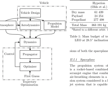
Fig. 1: Overview of the optimisation process

of 27.5◦.

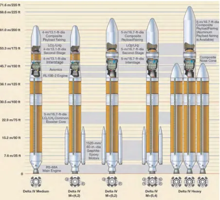
The Delta IV M is the smallest variant in the ULA Delta IV family of expendable launch vehicles (see Fig. 3). It is a single core vehicle, without boost-ers, which is powered by a RS-68A engine in the first stage, and an RL-10-B-2 engine in its upper stage. It is rated to deliver a 9190 kg payload to a 200 km alti-tude, circular orbit with an inclination of 28.5◦.11, 12

Table 1 displays the key mass parameters assumed in the study for both the spaceplane and the rocket. The published payload/orbit values by Olds et al. were generated assuming the trajectory followed a path of constant dynamic pressure and using an OMS to circularise the orbit. The trajectory used here for Hyperion was optimised using different system mod-elling software and an objective to minimise the re-quired fuel mass onboard. Using the same gross take-off weight (GTOW) and dry mass, a substantially larger payload was found, 24254 kg compared to 9072 kg, that could be delivered to the same orbit as the Delta IV.

II.I Propulsion

This section describes the details of the modelling approaches for the propulsion system including

emis-Hyperion Hyperion Delta IV (Olds et al.) (optimised)

Dry mass 61 439 61 439 30 780

Payload 24 254 9072* 9190

Propellant 277 498 292 680 224 401 Total Mass 363 191 kg 363 191 kg 292 680 kg *Rated to a different orbit: 160 km LEO ati= 27.5◦

Table 1: Mass budget of test vehicles to a 200 km LEO at 28.5◦ inclination

sions of both the spaceplane and the Delta IV. II.I.1 Spaceplane

The propulsion system of the Hyperion vehicle is a rocket-based combined cycle (RBCC) ejector-scramjet engine that combines rocket elements with air-breathing elements in a single unit. The propul-sion system considered is a LOX/LH2 ejector scram-jet system that is capable of operating in several modes: an rocket with ejector mode for low altitudes and velocities, high efficiency air-breathing ramjet and scramjet modes and as a rocket for higher alti-tudes and velocities. The averageIspof the resulting propulsion combination is higher than that of a tra-ditional expendable launch system, and enables the vehicle to be a single-stage-to-orbit vehicle.

The tool used to model this engine, HyPro, was developed and validated at Strathclyde by Mo-gavero.13–15 _{HyPro was developed as a fast and}

mod-ular software package for modelling combined-cycle propulsion systems for configurational engine opti-misation, multi-disciplinary design optimisation and system analyses. It uses a ’jump solver’ approach, where an engine is divided into components, and the analysis jumps in steps between the beginning of each component to the end. The choice of this method lends HyPro the flexibility to be able to model com-plicated and variable engine configurations. Other examples of propulsion codes that use this technique are the Ramjet Performance Analysis Code (RJPA) and SCCREAM16from Georgia Institute of Technol-ogy. EcosimPro, and its propulsion implementation ESPSS17 use a similar approach, albeit solving the models simultaneously instead of sequentially.

Fig. 2: Configuration of Hyperion Vehicle10

Fig. 3: Configuration of the Delta IV family11

HyPro was used to construct a surrogate model us-ing the MATLAB curve-fittus-ing tool for each propul-sion system as a function of altitude and Mach num-ber. This was done to increase the computational speed of the propulsion model, whilst maintaining an acceptable level of accuracy. The ramjet was fit with a (4,4) order bivariate polynomial, with a root-mean-squared-error of 6.95×104_{N and maximum error of}

4×105N. Similarly, the scramjet and the rocket were fit with (4,2) order polynomials, with mean-squared-errors of 1.895×104N and 833.7 N and maximum

er-Intake Freestream

Mixer Rocket

Diffuser Injector Phi

Combustor Nozzle

Thrust

Fig. 4: Hyperion engine architecture

rors of 1.9×104_{N and 6544 N respectively. A}

throt-tle, τ is applied directly to the resultant mass flow rate and thrust level of the engine,

FT =τ FT(surrogate) [1a]

˙

m=τm˙(surrogate). [1b]

II.I.2 Delta IV

The propulsion system for Delta IV rocket was mod-elled using a standard rocket equation model. The first stage utilises a RS-68A LH2/LOX rocket engine,

and the second stage uses a RL10-B-2 LH2/LOx

en-gine. The parameters of these engines used in this study are shown in Table 2.

Parameter RS-68A RL-10-B-2 Vacuum thrust 3560 kN 110 kN Vacuum ISP 414 s 465.5 s Mixture ratio 5.97 5.89

Table 2: Parameters of the Delta IV propulsion sys-tems

vacuum,

FT ,p=FT ,v−Aep(h) [2] where p(h) is the pressure at the current altitude,

FT ,v is the vacuum thrust, FT ,h is the thrust at the current altitude andAeis the exit area of the nozzle. II.I.3 Emissions Models

The H2O emissions released by both vehicles are

cal-culated based upon the mass flow rate at every time step of the integration. Since both vehicles use H2

and O2 propellent, the chemical equation governing

the mass of H2O produced is:

2 H2+ O2−−→2 H2O [3]

II.II Aerodynamics

The lift and drag forces are determined using the co-efficients of lift and drag and a single reference area for the vehicle.

L= cLρv

2_S

ref

2 [4a]

D=cDρv

2_S

ref

2 [4b]

centered whereρis the atmospheric density, v is the vehicle velocity, andSref is the vehicle reference sur-face area.

II.II.1 Spaceplane

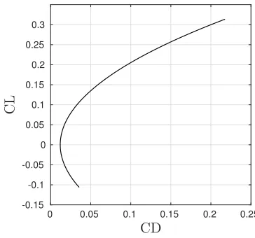
The aerodynamics of the spaceplane are modelled by calculating the coefficients of drag,cDand liftcLas a function of the Mach numberM and angle of attack

α of the vehicle. The curves for the the cD and cL are taken from Young et al.9 _{who further developed}

the Hyperion concept to create a secondary vehicle Lazarus. The mission profile of the vehicle was al-tered by using a sled-launch system, but the overall vehicle design was kept the same. The aerodynamics were calculated using the CBAERO software package and are shown in Fig. 5.

-10 0 10 20 30

Angle of Attack (deg) -4

-3 -2 -1 0 1 2 3 4

L/D

(a) Lift-to-Drag ratio as a function of the angle of attack

0 0.05 0.1 0.15 0.2 0.25 CD

-0.15 -0.1 -0.05 0 0.05 0.1 0.15 0.2 0.25 0.3

C

L

(b) Coefficient of lift against coefficient of drag

Fig. 5: Aerodynamic properties used in the space-plane trajectory optimisation9

II.II.2 Rocket

The aerodynamics of the rocket are modelled by ne-glecting the lift component and calculating the drag assuming a constant CD = 1, which is likely much higher than reality.18 _{However, the difference}

be-tween the angle of attack and the flight path is always zero in this model, i.e. the Sref is always the cross-sectional area of the rocket, so there is an additional drag component not accounted for here.

II.III Operating Environment

alti-tude,h. From these the air densityρand local speed of sound are calculated. This model divides the at-mosphere into layers, each has a linear temperature distribution with altitude. Both the pressure and the density are found by solving the vertical pressure vari-ation and the ideal gas law.

The Earth is modelled as a spherical, rotating planet with radius RE = 5 375 253 m and an angu-lar velocity of ωE = 7.292 115×10−5rad s−1. The Earth’s acceleration due to gravity is modelled as a function of altitude,

g= µE

r2 = µE

(h+RE)2 [5]

where the standard gravitational parameter, µE = 398 600.4418 km3_s−2_.

II.IV Flight dynamics and control

Both vehicles are considered to be a point with vari-able mass, centred at the centre of mass of the vehi-cle. The vehicle is flying around a spherical, rotat-ing Earth and the dynamics are therefore formulated with respect to a geocentric rotating reference frame using spherical coordinates.

The state vector of the vehicle is x = [h, λ, θ, v, γ, χ] wherehis the altitude,vis the veloc-ity in the Earth-centred Earth-fixed reference frame,

γ is the flight path angle, χ is the heading, λis the latitude,θis the longitude. The equations of motion are:19

˙

h= ˙r=vsinγ [6a]

˙

λ= vcosγsinχ

r [6b]

˙

θ= vcosγcosχ

rcosλ [6c]

˙

v= FTcos(α)−D

m −gsinγ [6d]

+ω2ercosλ(sinγcosλ−cosγsinχsinλ) ˙

γ= FTsin(α) +L

mv cosµ−

g

v − v r

cosγ [6e] + 2ω_ecosχcosλ

+ω2_er v

cosλ(sinχsinγsinλ+ cosγcosλ) ˙

χ= L

mvcosγsinµ− v

r

cosγcosχtanλ [6f] + 2ω_e(sinχcosλtanγ−sinλ)

−ω2_e

_r

vcosγ

cosλsinγcosχ [6g] wheremis the mass of the vehicle,FT is the magni-tude of the thrust from the engine,Land D are the

lift and drag of the aerodynamic forces on the vehi-cle, r=RE+hwhere RE is the Earth’s radius, ωE is the rotational velocity of the Earth, g is the ac-celeration due to gravity. The flight path angle γ is defined as being the angle between the local horizon and the velocity vector, and the flight heading angle

χis defined as the angle between north and the hori-zontal component of the velocity vector. The control law governs the angle of attack α, bank angleµand the propulsion throttle of the vehicle.

III TRAJECTORY OPTIMISATION The trajectory is determined using an in-house Space-plane Integrated Design Environment software.20–22

The approach uses flight segment decomposition technique with direct, multi-shooting transcription and solved with a local optimiser based on sequential quadratic programming and/or interior point meth-ods.

The flight phase decomposition approach allows the user to define any number of mission phases. Within each phase, the number of shooting elements, control nodes, system models, integration and inter-polation methods can all be specified. This allows for greater flexibility in configuring the problem, but does require knowledge of the system by the user. Discontinuities in the state and control variables are allowed by the system based on the matching condi-tions defined between each phase.

III.I Optimal Control

The optimal control problem is transcribed into an nonlinear programming (NLP) problem by using a multi-phase, multiple-shooting approach. The mis-sion is initially divided into np user-defined phases. Within each phase, the time interval is further di-vided intonmultiple shooting segments.

∪np

k=1∪

n−1

i=0[ti,k, ti+1,k] [7]

With each interval [ti,k, ti+1,k], the control is further

discretised into nc control nodes {ui,k0 , ..., u

i,k nc} and

collocated on Tchebycheff points in time.

Continuity constraints on the control and states are imposed,

xi,k=F([ti−1,k, ti,k],xi−1,k) ui−1,k

nc =u

i,k

0

fork= 1, ..., np [8] x1,k=x(tn+1,k−1)

u1₀,k=un_n+1_c ,k−1

where F([ti−1,k, ti,k],xi−1,k) is the final state of the

numerical integration on the interval [ti−1,k, ti,k] with initial conditionsxi−1,k. This approach increases the degree of freedom of the optimisation process reduc-ing the sensitivity of the overall problem to its vari-ables although at a cost of a steep increase in the number of optimisation variables.

The optimisation variables are therefore:

• The initial state vector of each shooting segment within every phase (excluding the first segment of the first phase)xi,k

• The control nodes of each shooting segment {ui,k₀ , ...,ui,knc}

• The time of flight for each shooting segment ∆ti,k

The discretised optimisation problem is defined as

min

{ui,k_j },{xi,k},{∆ti,k}

φ(xn,np)+

np

X

k=1

n−1 X

i=0

∆ti,kf0(xi,k,u i,k j ) [10] subject to

xi,k=F([ti−1,k, ti,k],xi−1,k),

uin−c1,k=u

i,k

0 ,

x1,k=x(tn+1,k−1),

u1₀,k=un_n+1_c ,k−1, c(x(t), u(t))≤0, t∈[t0, tf]

g(xn,k,un,k_nc)≤0, ω(x0,1,xn,np) = 0

fori= 1, ..., n−1,k= 1, ..., np and ∆ti,k =ti+1,k−

ti,k. Path constraints are evaluated at a discrete set of points based in time, andg(xn,k,un,knc ) are the

in-equality constraints for phase switching. III.II Optimisation Algorithm

The NLP problem is solved using the local interior-point optimisation in MATLAB’sfminconfunction.

One of the major limitations of trajectory optimi-sation is the need to produce good first guesses of the trajectory. Both convergence and the optimal-ity of the final solution are heavily dependent on the first guess. Both a user-input first guess control law, or a global-search optimisation can be used to gen-erate this. The former could be previous trajectory data, an expected result or a designed solution (for example, taking into account the optimal regime of the propulsion system). Alternatively, the user could

input a constant control law. The second method is to use a stochastic global search to quickly survey the entire survey space. A constant control law was chosen as the first guess for all optimisations in this paper.

IV TEST CASE IV.I Spaceplane

The test case chosen was a mission to launch a pay-load to 28.5◦ 200 km orbit, as if it were taking off from the Kennedy Space Center. The trajectory has three propulsion models applied, the ramjet, scram-jet and rocket. The time, velocity and altitude at which switching between them occurs has not been constrained. The control parameters for the ascent trajectory are c= [α, τ, ttof], where ttof is the time of flight of each phase. The control law is discrete, and characterised by a number nodes in each phase distributed using a Chebyshev distribution for each phase. The control is interpolated between these points using a Piecewise Cubic Hermite Interpolat-ing Polynomial, written as a fast Matlab-generated MEX function.

The control space is constrained by the following bounds: α∈[−10◦,30◦] andτ ∈[0.8,1] for the ram-jet and scramram-jet phases, andτ ∈[0.6,1] for the rocket phases. There are five phases in total, two each for the ramjet and scramjet propulsion systems, and one for the rocket phase. The ramjet and scramjet phases each have 4 control nodes, and the rocket phase has 10 control nodes. The time is constrained to a maxi-mum of 300 s for the ramjet and scramjet phases, and 500 s for the rocket phase.

The initial parameters for the state vector are:

h(t= 0) = 8 km

v(t= 0) = 900 m s−1

γ(t= 0) =λ(t= 0) =χ(t= 0) = 0◦

φ(t= 0) = 27.5◦

m(t= 0) = 325 000 kg

[11]

where the altitude, velocity and mass are calculated based upon the flight profile Hyperion. There are no constraints applied to phases, and therefore the time at which the vehicle switches will purely be a function of the models.

objective function is min

c∈Dmp(t=tf). [12] Additional constraints are placed on the maximum vehicle acceleration in both the longitudinal and nor-mal axis of the vehicle ofax, az ≤3g0m s−2 and on

the maximum dynamic pressure of the vehicle during flightq= 1₂ρv2≤300 000 Pa.

IV.II Delta IV

The Delta IV trajectory was reconstructed by propa-gating over a trajectory using the vehicle and system models described in section II. MATLAB’sode45 in-tegrator, which is based on an explicit Runge-Kutta (4,5) formula, the Dormand-Prince pair was used for this. A time-based control law was applied for the flight path angle, γ of the rocket during flight, The throttle,τ was assumed to be 1 unless the rocket ex-ceeded an acceleration limit, when the throttle would be reduced. This acceleration limit was based on the acceleration environment described in the Delta IV User Manual. The rate of change of the flight path angle was adjusted until the resultant trajectory matched the known trajectory points of the vehicle described in the ULA Users Manual. As this study is investigating the altitude distribution of emissions, the most important parameter curves to match were the altitude vs. time/downrange profiles, and the mass to orbit.

IV.III Results

The result of the trajectory optimisation for the spaceplane is a trajectory that achieves the requested orbited and all other constraints - and has a fi-nal burnout mass of 85 692 kg, including the pay-load mass. This results in a paypay-load mass of around 24 254 kg, over twice that of the reference Hyperion vehicle given in Olds et al. There are a number of possible reasons for the discrepancy. There are un-certainties in the models used within this simulation, as well as those in the reference papers. HyPro in particular predicts higher thrusts and specific im-pulses compared with the SCCREAM solver, al-though Mogavero suggests that HyPro matches other data sources.15 _{Perhaps the most likely reason is that}

the trajectory presented here is an optimal solution, although probably not the global solution. The tra-jectory produced by Olds was assumed to be flying along the propulsion-optimal constant dynamic pres-sure trajectory, and is unlikely to be vehicle-optimal for this reason.

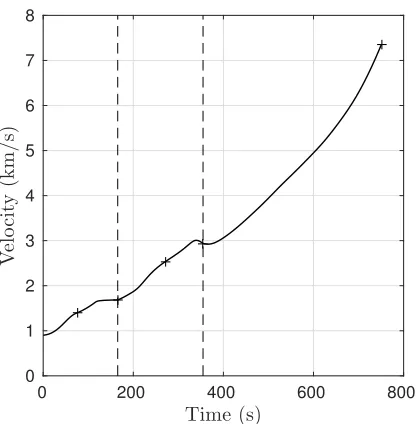
The key flight parameters are shown in figs. 6 to 9, and the trajectory is combined with emissions data in fig. 10. Figure 6 shows the flight path angle of the trajectory, and the angle of attack used to produce this trajectory, which stays within the bounds. The thrust curve in fig. 8 shows how the thrust varies with time through the flight. The throttle can be discon-nected between phases, which is why the thrust isn’t continuous and connected. One of the constraints that was applied to this optimisation was the dy-namic pressure, at 2×105_{Pa, whereas Hyperion flew}

on a 95 760 Pa dynamic pressure boundary. The ram-jet has an operational range of 2.5 ≤M ≤ 6 whilst the scramjet has an operational range of 5≤M ≤10. The point at which the vehicle switched propulsion systems is chosen by the optimiser, in this case the vehicle switched from ramjet to scramjet at mach 5.7, and from scramjet to rocket at mach 9.8.

Figure 10 shows a direct comparison between the Delta IV and the spaceplane. Both the trajectory (al-titude vs. time) and the mass flow rate of H2O with

time are plotted. The H2O released by the spaceplane

is much higher than that of the Delta IV, since the propellant carried on board the spaceplane for the air-breathing phase is all hydrogen. For the space-plane, 5.0143×105kg of H2O was generated along

the trajectory, and 2.24×105kg by the Delta IV. The amount H2O produced by its first propulsion system,

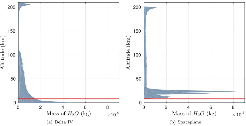
the ejector, hasn’t been included in this total, so the amount produced by the spaceplane is significantly higher. Figure 11 shows the altitude distribution over which this H2O was released. The altitude region in

which the emitted H2O peaks is between 20 - 30 km,

the area of the lower stratosphere where the ozone layer exists. The Delta IV on the other hand does not spend much time in this region of the atmosphere, as it is still under power from the first stage, and a large amount of its time of flight is spent at altitude increasing its velocity to orbital velocity.

V CONCLUSIONS

This paper has outlined an approach for investigat-ing the emissions of transatmospheric vehicles, in this case an expendable launch vehicle and a spaceplane concept. The scenario explored investigates the en-vironmental impact of an ascent trajectory of both of these vehicles to a 200 km 27.5◦ orbit. The results show that higher amounts of H2O are dispersed into

0 200 400 600 800

Time (s)

-10 -5 0 5 10 15 20 25 30

A

n

g

le

(d

eg

)

FPA AoA

Fig. 6: Both the flight path angle and the angle of attack are plotted in this figure. The circles on the angle of attack line represent the control nodes from which the control law is interpolated. The dotted lines represent the propulsion switches.

0 200 400 600 800

Time (s) 0

0.4 0.8 1.2 1.6 2

D

y

n

a

m

ic

P

re

ss

u

re

(P

a

)

×105

Fig. 7: Dynamic Pressure of the Hyperion space-plane during the flight. A maximum constraint of 2×105Pa was applied. Dotted line indicates the change in propulsion system.

0 200 400 600 800

Time (s) 0

1 2 3 4 5

T

h

ru

st

(N

)

×106

Fig. 8: The thrust of the Hyperion vehicle during the flight. The influence of this on the Mass Flow of H2O is apparent. Dotted line indicates the change

in propulsion system.

0 200 400 600 800

Time (s)

0 1 2 3 4 5 6 7 8

V

el

o

ci

ty

(k

m

/

s)

0 400 800 1200

Time (s) 0

200 400 600 800 1000 1200 1400 1600

M

a

ss

F

lo

w

o

f

H2

O

(k

g

/

s)

0 50 100 150 200 250

A

lt

it

u

d

e

(k

m

)

(a) Delta IV

0 400 800 1200

Time (s) 0

200 400 600 800 1000 1200 1400 1600

M

a

ss

F

lo

w

o

f

H2

O

(k

g

/

s)

0 50 100 150 200 250

A

lt

it

u

d

e

(k

m

)

(b) Spaceplane

Fig. 10: Comparison of Delta IV and Spaceplane mass flow rate of H2O emissions with time. The red line

indicates the trajectory (altitude with time). The area highlighted in blue represents the total emissions from each launch vehicle.

0 2 4 6 8

Mass ofH₂O _(kg)

×104 0

50 100 150 200

A

lt

it

u

d

e

(k

m

)

(a) Delta IV

0 2 4 6 8

Mass ofH₂O _(kg)

×104 0

50 100 150 200

A

lt

it

u

d

e

(k

m

)

(b) Spaceplane

Fig. 11: Comparison of Delta IV and Spaceplane mass of H2O emissions with altitude. The red line indicates

between 20 - 30km. At this altitude range H2O can

have a major impact on ozone depletion.

Future work could include improving the launch vehicle atmosphere interaction, by modelling impor-tant phenomena like the plume and combustion after the exhaust exit. This methodology can also be ex-tended to cover other trajectories or vehicles, includ-ing point-to-point supersonic and hypersonic trans-portation and other launch vehicles. It can be fur-ther extended to investigate ofur-ther emissions, such as NOx, CO2, CO and SO2 and propellant types such

as kerosene, methane or solid propellants. It can also be integrated into a design platform for vehicle con-cepts, extending the multidisciplinary design process from solely performance and operational objectives to include environmental concerns.

REFERENCES

[1] Varvill, R. and Bond, A., “A Comparison of Propulsion Concepts for SSTO Reusable Launchers,” Journal of the British Interplane-tary Society, Vol. 56, 2003, pp. 108–117. [2] Ross, M., Toohey, D., Rawlins, W., Richard,

E., Kelly, K., Tuck, A., Proffitt, M., Hagen, D., Hopkins, A., Whitefield, P., et al., “Observation of stratospheric ozone depletion associated with Delta II rocket emissions,”Geophysical research letters, Vol. 27, No. 15, 2000, pp. 2209–2212. [3] Ross, M., Danilin, M., Weisenstein, D., and Ko,

M. K., “Ozone depletion caused by NO and H2O emissions from hydrazine-fueled rockets,” Journal of Geophysical Research: Atmospheres, Vol. 109, No. D21, 2004.

[4] Brady, B., Martin, L., and Lang, V., “Effects of launch vehicle emissions in the stratosphere,” Journal of spacecraft and rockets, Vol. 34, No. 6, 1997, pp. 774–779.

[5] Ross, M., Toohey, D., Peinemann, M., and Ross, P., “Limits on the space launch market related to stratospheric ozone depletion,”Astropolitics, Vol. 7, No. 1, 2009, pp. 50–82.

[6] Liu, S. K., Aerospace-Plane Flights and Strato-spheric Ozone: Review and Preliminary Assess-ment of the National Aerospace Plane (NASP) Operations, Vol. 3464, Rand Corporation, 1992. [7] Grooß, J.-u., Br¨uhl, C., and Peter, T., “Im-pact of aircraft emissions on tropospheric and

stratospheric ozone. Part I: Chemistry and 2-D model results,” Atmospheric Environment, Vol. 32, No. 18, 1998, pp. 3173–3184.

[8] Olds, J. R. and Bradford, J., “SCCREAM (Sim-ulated Combined-Cycle Rocket Engine Analy-sis Module): A conceptual RBCC engine design tool,”Joint Propulsion Conference, 1997. [9] Young, D. A., Kokan, T., Clark, I., Tanner,

C., and Wilhite, A., “Lazarus: A SSTO Hy-personic Vehicle Concept Utilizing RBCC and HEDM Propulsion Technologies,” International Space Planes and Hypersonic Systems and Tech-nologies Conference, AIAA, 2006.

[10] Olds, J., Bradford, J., Charania, A., Ledsinger, L., McCormick, D., and Sorensen, K., “Hype-rion: an SSTO vision vehicle concept utilizing rocket-based combined cycle propulsion,”AIAA paper, 1999, pp. 99–4944.

[11] ULA, “Delta IV Launch Services Users Guide,” Tech. rep., United Launch Alliance, 2013. [12] “Space Launch Report - Delta IV,” http:

//www.spacelaunchreport.com/delta4.html, Accessed: 2016-09-07.

[13] Mogavero, A. and Brown, R. E., “An improved engine analysis and optimisation tool for hyper-sonic combined cycle engines,” AIAA Interna-tional Space Planes and Hypersonic Systems and Technologies Conference, 2015.

[14] Mogavero, A., Taylor, I., and Brown, R. E., “Hy-brid Propulsion Parametric and Modular Model: a novel engine analysis tool conceived for design optimization,”AIAA International Space Planes and Hypersonic Systems and Technologies Con-ference, Atlanta GA, 2014, pp. 16–20.

[15] Mogavero, A.,Toward automated design of Com-bined Cycle Propulsion, Ph.D. thesis, University of Strathclyde, 2016.

[16] Olds, J. R. and Bradford, J. E., “SCCREAM: a conceptual rocket-based combined-cycle engine performance analysis tool,” Journal of Propul-sion and Power, Vol. 17, No. 2, 2001, pp. 333– 339.

[18] Naughton, J. W., “Reduction of Base Drag on Launch Vehicles,” 2002.

[19] Tewari, A.,Atmospheric and space flight dynam-ics, Springer, 2007.

[20] Ricciardi L, Toso F, V. M. M. C., “Multi-objective optimal control of the ascent trajecto-ries of launch vehicles,”Astrodynamics Specialist Conference, AIAA Space and Astronautics Fo-rum and Exposition, 2016.

[21] Toso, F., Maddock, C., and Minisci, E., “Opti-misation of Ascent Trajectories for Lifting Body Space Access Vehicles,” Space transportation solutions and innovations symposium, Interna-tional Astronautical Congress, 2015.