City, University of London Institutional Repository
Citation
:
Paraskevopoulos, D. C., Tarantilis, C. D. & Ioannou, G. (2016). An adaptive memory programming framework for the resource-constrained project scheduling problem. International Journal of Production Research, 54(16), pp. 4938-4956. doi:10.1080/00207543.2016.1145814
This is the accepted version of the paper.
This version of the publication may differ from the final published
version.
Permanent repository link: http://openaccess.city.ac.uk/19847/
Link to published version
:
http://dx.doi.org/10.1080/00207543.2016.1145814Copyright and reuse:
City Research Online aims to make research
outputs of City, University of London available to a wider audience.
Copyright and Moral Rights remain with the author(s) and/or copyright
holders. URLs from City Research Online may be freely distributed and
linked to.
To appear in theInternational Journal of Production Research
Vol. 00, No. 00, 00 Month 20XX, 1–21
An Adaptive Memory Programming framework for the Resource Constrained Project Scheduling Problem
Dimitris C. Paraskevopoulosa∗, Christos D. Tarantilisband George Ioannoub
aSchool of Management, University of Bath, Claverton Down, Bath, BA2 7AY, UK;
bDepartment of Management Science & Technology, Athens University of Economics & Business, 76
Patission Str., GR10434
(Received 00 Month 20XX; final version received 00 Month 20XX)
The Resource Constrained Project Scheduling Problem (RCPSP) is one of the most intractable combi-natorial optimisation problems that combines a set of constraints and objectives met in a vast variety of applications and industries. Its solution raises major theoretical challenges due to its complexity, yet presenting numerous practical dimensions. Adaptive Memory Programming (AMP) is one of the most successful frameworks for solving hard combinatorial optimisation problems (e.g., vehicle routing and scheduling). Its success stems from the use of learning mechanisms that capture favourable solution elements found in high quality solutions. This paper challenges the efficiency of AMP for solving the RCPSP, to our knowledge, for the first time in the up-to-date literature. Computational experiments on well known benchmark RCPSP instances show that the proposed AMP consistently produces high-quality solutions in reasonable computational times.
Keywords:Adaptive Memory Programming, Project Scheduling, Resource Constraints
1. Introduction
Scheduling activities under the consideration of particular resource capacity and precedence con-straints is a major complex scheduling problem faced in several different industries. Hartmann and Briskorn (2010) discuss on scheduling applications that can be modelled as Resource Constrained Project Scheduling Problem variants and extensions. Shop scheduling environments, sports league scheduling, scheduling of port operations, scheduling of multi-skilled workforce and school and university timetabling is only a sample of the RCPSP’s vast range of applications (Hartmann and Briskorn 2010). The RCPSP model is hence not restricted only in its original field, that is project scheduling, but also addresses major scheduling problems faced in different industries.
The RCPSP can be described as follows. Let a single project consist of a set of activitiesJ that must be executed to complete the project. Precedence constraints do not allow an activity i to start before all its immediate predecessors have finished. There exists a set of resources K with limited capacity, used for the execution of the activities. Each activity i has its own predefined durationdi and spends a specific amount of resource units for its execution rik, for each resource
k∈K. The goal is to find the resource and precedence feasible finish times of the activities, such that the finish timeln+1 of the last activity is minimised.
According to Garey and Johnson (1979), the RCPSP is one of the most intractable combinatorial optimisation problems and belongs to theNP-hard class of problems (Blazewiczet al. 1983). Due to its complexity, as well as its practical interest, the RCPSP has attracted much attention by
∗Corresponding author. Email: [email protected], Tel: +441225386233, Co-authors: Christos D. Tarantilis Email:
researchers in the latest decades (Hartmann and Briskorn 2010; Kolisch and Hartmann 2006). Although there are significant achievements in the field of exact methods (see Zhu et al.2006 for the multi-mode RCPSP and Brucker et al. 1998, Zamani 2001 and Demassey et al 2005 for the single mode RCPSP) the literature still favours metaheuristics for solving realistic scale problem instances. One of the most successful metaheuristic frameworks for solving hard combinatorial optimisation problems is Adaptive Memory Programming. AMP has produced the best-known results for major vehicle routing problems (Repoussiset al. 2010; Tarantilis et al.2014; Gounaris
et al.2014) and binary quadratic programs (Glover et al.1998), and has been applied for solving, among others, supply chain design problems (Cardona-Valdeset al.2014; Velarde and Marti 2008). Inspired and motivated by this stream of research, this paper contributes to the existing body of work by introducing for the first time in the RCPSP literature an AMP framework for solving the RCPSP. The proposed AMP combines memory structures to capture favourable solution elements and in this way produce high quality solutions. Specifically, the adaptive memory monitors the scheduling habits of the activities and the AMP framework uses this information to guide the search towards promising and unexplored regions of the solution space. To achieve this goal, our AMP consorts with a Greedy Randomised Reconstruction (GRR) method and a powerful local search algorithm in the spirit of Variable Neighbourhood Search (Paraskevopoulos et al. 2008). The resulting AMP framework was tested on large scale and well-known benchmark instances and outperformed the state-of-the-art of the literature under 1000 and 5000 schedules examined, while remaining highly competitive when 50000 schedules are examined.
The remainder of this paper is organised as follows. Section 2 discusses the relevant literature mainly focusing on the AMP and the RCPSP domains. Section 3 presents the solution methodology and describes in detail all components. Computational experience is presented in Section 4. Finally, conclusions and further research directions are discussed in Section 5.
2. Literature Review
In this section, we first present the relevant Adaptive Memory Programming literature and then talk about the recent developments on metaheuristics for solving the RCPSP.
Adaptive Memory Programming is a general-purpose solution framework that focuses on the exploitation of strategic memory structures (Glover 1997). The main goal is to capture common solution characteristics met in the search history and use this information to produce high quality solutions. This non problem-specific rationale enabled the successful application of AMP frame-works for solving a large variety of hard combinatorial optimisation problems.
Gloveret al.(1998) developed an adaptive memory tabu search (AMP-TS) algorithm for solving binary quadratic programs that model various combinatorial optimisation problems. The proposed AMP-based TS collects information from the local optima throughout the search trajectory, i.e., captures each time a local move causes the objective function to increase or remain unchanged. Recency and frequency information are combined to guide effectively the search to new directions into the solution space. Computational experiments indicate the effectiveness and efficiency of the proposed solution methodology.
Cardona-Valdeset al.(2014) consider the design of a two-echelon production distribution network with multiple manufacturing plants, distribution centres and a set of candidate warehouses. Their contribution is threefold a) the consideration of the demand uncertainty regarding the warehouse location problem, b) the focus on both economical and service quality objectives and an AMP-TS to address the underlying bi-objective stochastic optimisation problem. Similar to the supply chain design problem, Velarde and Marti (2008) applied an AMP framework for solving the supplier selection problem in an international setting under uncertainty in the macroeconomic conditions of the associated countries. The proposed AMP uses memory structures to discourage the selection of frequently selected suppliers and preserve a balance between intensification and diversification. Vehicle routing problems have attracted much attention on the development of efficient AMP frameworks. The latter have produced the best-known results when tested on well-known bench-mark problems of classical and rich vehicle routing variants (Repoussis et al. 2010; Tarantilis et al.2014). Gounaris et al.(2014) presented an AMP framework to address the robust capacitated vehicle routing problem. Subroutes of the elite set of solutions represent the favourable solution elements and constitute the information stored in the adaptive memory. These subroutes are of varying size and are combined to create new provisional solutions.
To our knowledge, there is not any metaheuristic framework in the RCPSP literature that ex-plicitly utilises adaptive memory structures within a solution framework. Nevertheless, there is a wide variety of metaheuristics for solving the RCPSP, which we discuss in the following.
Debels and Vanhoucke (2007) presented a decomposition-based Genetic Algorithm (GA) for solving the RCPSP. The proposed algorithm selects a time window of the RCPSP schedule and extracts the associated activities to this time window. A sub-problem is constructed and solved via an efficient GA. The improved subproblem solution is embedded into the main solution in a way to improve the makespan. More recently, Zamani (2013) proposed a GA that used a a specialised crossover operator that combines two coherent parts from one parent and one part from the other. The order of these parts change but they still remain contiguous. The author assumes that contiguity of the parts matters to preserve the fitness of their both parents. Computational experiments indicate the effectiveness of the method.
Swarm Intelligent (SI) population based algorithms have been also developed for solving the RCPSP. The latter are nature inspired procedures that emulate the behaviour of several species such as ants, bees and birds. Merkle et al. (2002) presented an Ant Colony Optimisation (ACO) algorithm for solving the RCPSP. Their algorithm uses an Activity List (AL) representation, while a Schedule Generation Scheme (SGS) is employed both in parallel and serial fashion to produce feasible schedules. Two pheromone strategies for the ant’s decisions are integrated.
Another algorithm that falls into the SI category of population based algorithms is the Particle Swarm Optimisation (PSO). PSO is an evolutionary algorithm that emulates the behaviours of birds flocking. Zhang et al. (2006) applied a PSO solution framework for addresing the RCPSP. The proposed PSO algorithm operates on a priority-based particle representation which resembles the Random Key (RK) representation and ensures that feasible activity sequences, in terms of precedence constraints, are considered. The proposed PSO utilizes a parallel SGS to transform the particles information to feasible schedules. Lately, Chen (2011) proposed a “justification” PSO (jPSO) that enables a technique to adjust the starting times of each activity in an effort to reduce the makespan. The resulting jPSO operates on both forward and backward planning schemes.
Regarding Scatter Search (SS) implementations, a hybrid methodology was proposed by Debels
proposed by Paraskevopouloset al.(2012). Our proposed AMP contributes to the existing body of work by introducing an adaptive memory-based solution reconstruction procedure, able to produce high quality solutions even in early stages of the search process; note that the proposed AMP outperforms the state-of-the-art of the literature for large scale RCPSP instances when 1000 and 5000 schedules are examined. Furthermore, an innovative local search method is presented that performs a thorough exploration of the solution neighbourhoods.
3. Solution Methodology
In this section, we first present the solution representation used by all the components of the algorithm and then describe in detail the components of the main algorithm.
3.1 The event-list representation
The most popular representation schemes of the literature is the activity list and the random key representation (Kolisch and Hartmann 2006). The main problem that typically occurs when these representations are used, is that multiple representation lists (either ALs or RKs) can be associated with the same solution (Debels and Vanhoucke 2007). The latter is expected to reduce the efficiency of metaheuristic methodologies, since useless replicas of the same solution exist in the solution space and therefore the search is typically delayed and misguided. Debels and Vanhoucke (2007) used several transformation mechanisms and a Standardized RK representation scheme that addressed the aforementioned problem. The Event List representation used in this paper (Paraskevopoulos
et al. 2012) addresses the inefficiencies of the AL and RK without the use of transformation mechanisms. The structure of the EL involves time information and efficiently depicts the RCPSP solution. Two different ELs cannot be associated with the same schedule/solution as they are composed by sets of activities that start at the same time, i.e., the events, while these events are ordered according to their starting times. If either the events or the order of these events, or both are different in two particular event lists, different solutions are considered. This property of the EL representation enables both local search to move effectively into the solution space, as well as it equips evolutionary algorithms with an efficient inheritance process. In this paper, we took advantage of the particular structure of the EL, and we introduce compound local search moves that consider “event relocations” within the schedule.
Figure 1 illustrates a project of 16 activities and a capacity-limited resource. The numbers, that appear on thexaxis in Figure 1b and in the event list, indicate the starting times, i.e., the dates of the events. The resource consumption and duration of the activities are shown in Figure 1b. The latter shows a feasible solution of the problem, obtained by using a serial SGS.
3.2 The objective function
A hierarchical objective function is used, inspired by Paraskevopouloset al. (2012). The primary objective is the makespan, and the secondary objective is a measure that mainly represents the deviation of the finishing timeslsj of the activities j in a solution sfrom their Earliest Finishing
Times (EF Tj) lower bounds calculated by the Critical Path Method (CPM). Typically, the largest
this deviation is, the less is the quality of a solution, when comparing two solutions with the same makespan. The equation below gives the hierarchical objective function used in this paper:
f(s) =min(ls(n+1),
∑ j∈J
lsj−EF Tj
EF Tj+1
|J| ) (1)
(a) Project Network (b) Typical RCPSP schedule
[image:6.595.123.473.56.297.2](c) Event list representation
Figure 1. A typical Resource Constrained Project Scheduling Problem
setJ, i.e., the number of activities.
This is a common practice in the relevant literature (Mendeset al. 2009), as the solution space is largely composed by solutions with the same makespan (Czogalla and Finik 2009), and this hierarchical objectives typically help the search to move within the space more effectively.
3.3 The Adaptive Memory Programming Framework
The proposed AMP consists of two phases; the initialisation and the exploitation phase. In the ini-tialisation phase a construction heuristic is applied for λiterations, throughout which µ different and good quality solutions are selected to comprise the set M. This pool of solutions M informs the adaptive memory α, which stores the scheduling history for each activity. In the exploitation phase, The AMP framework manipulatesM through an exploration of search trajectories initiated from new provisional solutions. In particular, a GRR method (Kontoravdis and Bard 1995) uses the information stored in the adaptive memory and produces a provisional solution s. Given s, a Reactive Variable Neighbourhood Search (ReVNS) algorithm is applied for improving the solu-tion quality. If the provisional solusolu-tionsis “sufficiently” improved through the application of the ReVNS, i.e., the provisional solution satisfies some elitist selection criteria, the pool of solutions is updated with the new, improved by ReVNS, solutions′ and the worst cost solution is removed from the pool. At this point, the adaptive memory is updated as well. The AMP continues with another provisional solution (whether the previous solution was improved or not) until the termination criteria are met. The AMP framework is described by Algorithm 1. The algorithm terminates after a number of schedulesmaxSc has been examined.
Algorithm 1:Adaptive Memory Programming Framework
Input:λ(initial population size), µ (pool size), whereλ≥µ,δ (number of local search iterations without an improvement), ϑmax (number of perturbations without an improvement), δt(size of the time bucket)
Output:M,sbest∈M
***Initialization Phase***
M←ConstructionHeuristic(µ, λ);
α←InitialiseAdaptiveMemory(M,δt) ; RCLsize = 1;
***Exploitation Phase***
whileNumber of schedules examined are less or equal to maxSc do
s← GRR(α, RCLsize);
s∗ ← ReV N Sdist(s, δ/2, ϑmax);
(s′, ⃗h)←ReV N Scost(s∗, δ, ϑmax);
if SelectionCriteria(M, s′)then
UpdatePool(M, s′);RCLsize = 1; α← UpdateAdaptiveMemory(M, s′, δt) ;
else
if RCLsize < µ then
RCLsize=RCLsize+ 1;
else
RCLsize= 1;
3.4 Initialisation Phase
The initialisation phase aims at producing an initial population of solutions that are both diver-sified and of good quality. A construction heuristic is proposed that combines a serial SGS with a backward, a forward and a bidirectional planning schemes. At each iteration of the initialisation phase, the planning scheme is selected at random with equal probability and is preserved until all activities are scheduled and a complete solution is constructed. The activity to be scheduled at a particular iteration is selected at random from all precedence feasible activities at that iteration. The construction heuristic is applied repeatedly untilλdifferent solutions are created, among which µare selected to build the poolM. Details about the creation of the pool of solutions are given in Section 3.4.2. The initial population is exploited in the exploitation phase.
3.4.1 The adaptive memory
A major element of the proposed algorithm is the adaptive memory α, which records the track of the search to identify favourable time buckets for each activity and guides the search towards high quality solution regions. The main intuition behind this strategy is that frequently visited solution elements (favourable time buckets in this instance) can be possibly found in optimum or higher quality solutions, especially if these elements belong to high quality solutions (Tarantilis 2005; Repoussiset al. 2010).
To capture the favourable solution elements appropriate memory structures are used. Taking advantage of the event-list representation structure the time information needed is easily extracted and stored in a two dimensional arrayα, i.e., the adaptive memory. To create the arrayα, the time horizon T is divided into T b= T /δt time buckets and the size of α is |J| ×T b, where |J| is the number of activities andδt the size of the time bucket in time units.
Initially, all the elements{i, t}of α are set equal to 0. In the initialisation phase,α is initialised with the information included in the pool of solutionsM. In particular, each element{i, t} ofα is incremented bybs, if activity iis scheduled at time bucket t and belongs to solution s∈M. The
wheref(s) is the primary objective as defined by equation (1). The higher the cost of a solutions, the lower is thebsand thus the lower is the impact of the solution elements of sinto the formation
of the adaptive memory. The latter is calculated according to the equation given below:
α(i, t) = ∑
s∈M
bsIits,∀i∈J,∀t∈ {1, ..., T b} (2)
whereirepresents an activity in solution sand Iits is a binary variable equal to 1 if activityiis scheduled within the time buckett, i.e., (t−1)δt≤STsi ≤tδt, where STsi is the starting time of
i, and 0 otherwise. Every time, a new solution is inserted into the pool of solutions,α is updated by using the procedure described above. Note that only the activity’s starting time STsi needs to
be (or equally the finish timelsi for the backward scheduling scheme) stored within the respective
time bucket, and not the whole execution time interval of the activity.
3.4.2 The selection criteria
The pool of solutions and the adaptive memory α are updated if certain criteria are met. The goal is to maintain a balance between quality and diversity and to avert premature convergence. Our diversity measure uses the distance measure of Chenet al.(2010b) between pairs of solutions, D(s, s∗) = ∑j∈J|lsj−ls∗j|, for two solutions s and s∗, where lsj and ls∗j are the finish times of
activityjin solutionssands∗, respectively,J is the set of activities andM is the pool of solutions. The total dissimilarity for poolM is then given by:
TD(M) = ∑
s,s∗∈M
D(s, s∗), (3)
where the sum is over allµ(µ−1)/2 pairs of solutions in setM.
The creation of the initial pool of solutions proceeds as follows. The firstµsolutions among the λgenerated within the Initialisation phase are inserted intoM. The remainingλ−µsolutions are then considered sequentially for replacing a solution inM. Specifically, if such a solutionssatisfies the conditionf(s) < f(sbest), where sbest is a least cost solution in M, or if f(s) < f(sworst) and TD(M) <TD(M \ {sworst} ∪ {s}), thens is inserted into M. Otherwise, s is not included in M. When s is inserted, solution sworst ∈M, where sworst has the largest cost among the solutions in M, is removed fromM. Note that, as soon as the pool of solutions is updated with a new solution, the adaptive memory is updated as well. The same rationale is followed in theExploitation Phase.
3.5 Exploitation Phase
The initial population is exploited in the second phase of AMP, the exploitation phase. In the following, the components of the exploitation phase are presented.
3.5.1 The greedy randomised reconstruction method
The way the information is extracted from the adaptive memory, is crucial and affects the efficiency and effectiveness of the proposed solution methodology. The information stored in the adaptive memory, is extracted by using a greedy randomised rationale (Kontoravdis and Bard 1995), which adaptively selects the information according to the track record of the search history.
For this purpose, a list, namely the Random Candidate List -RCLi, is used to store the highest
score elements α{i, t} of activity i, ∀t ∈ {1, ..., T b}. Each activity i is assigned with its own list RCLi. The size of the list is dynamic and starts from 1 and increases as no improvement in the
is found the RCL size is reinitialised to 1, for intensification purposes. Details on how the RCL size is controlled are given in Algorithm 1.
The provisional solution is built step by step, by scheduling one activity at a time. Starting from an empty schedule, a set A of precedence feasible activities is created. The first activity to be scheduled is the activity that has the highest score α∗{i, t}, i.e., maxi∈A{α∗{i, t}}, among all the
precedence feasible activitiesi∈ A. The scoreα∗{i, t}is derived by selecting at random one of the elements of the list RCLi. Also, the element α∗{i, t} provides the favourable time bucket t∗i that
activityishould be scheduled.
A scheduling procedure tries then to schedule the activityias close as possible to the desirablet∗i without violating any resource capacity constraints. Note that, it is not always possible to schedule all the activities to their favourable time buckett∗i due to the resource constraints and due to the serial nature of the scheduling procedure and they are thus scheduled as close as possible to their t∗i. As soon as activity iis scheduled, it is removed from the setA, set A is populated with more precedence feasible activities and the procedure iterates until A is empty, i.e., all activities i∈J have been scheduled.
To illustrate the mechanics of the adaptive memory and the reconstruction procedure we pro-vide the following example. Assume the problem instance of Figure 1 and a pool of solutions with size µ = 9. The time horizon T is set equal to 40 and divided in time buckets of size δt = 5, thus the number of time buckets is T b = T /δt = 8. The adaptive memory α has a size of 18x8, compliant with the 18 activities and the 8 time buckets available. Assume also that, after some iterations of the reconstruction mechanism, some of the activities have already been scheduled. Then, on a particular iteration, set A contains activities 16, 10 and 9 and the size of RCL is equal to 2. Assume also that the adaptive memory records of these three activities are α{9, t} = {0,0,0.345,0.546,0.034,0,0}, α{10, t} = {0,0,0.897,0.098,0,0.023,0}, α{16, t} =
{0,0,0.054,0.345,0.245,0,0}, witht∈ {1, ...,8}. Given all this information, the RCLs are created. Because the RCL size is equal to two, the two highest score elements of each α{i, t} are selected. Therefore the following RCLs are created: RCL9 = {0.546,0.345}, RCL10 = {0.897,0.098} and RCL16 ={0.345,0.245}. Next step, an element of RCLi for eachi is selected at random. Let the
following elements be the selected ones:α∗{9, t}= 0.345,α∗{10, t}= 0.897 and α∗{16, t}= 0.345, and the respectivet∗is are,t∗9 = 3,t∗10= 3, and t∗16= 4.
Among the three activities, the activity that has the highest score α∗{i, t} is activity 10, and will be scheduled next. Specifically, activity 10 will be scheduled as close as possible to time bucket 4, i.e., the time interval from 15 to 20 (from (4-1)×δt to 4×δt, δt=5) within the time horizon, without violating any resource capacity constraints. Then activity 10 is removed from setA, more precedence feasible activities are inserted into A and the procedure continues by comparing the adaptive memory records of the activities in the updated setA, until all activitiesi∈J have been scheduled.
3.6 The reactive variable neighbourhood search
The provisional solution produced by the reconstruction method is subject for improvement by a ReVNS. The basic idea of the variable neighbourhood local search is the systematic change of neighbourhoods within local search (Paraskevopoulos et al. 2008). The systematic change of the neighbourhood is following an increasing cardinality scheme, such that small neighbourhoods are chosen initially and as an improvement in the solution quality is not observed, the neighbourhood cardinality is increased by selecting different neighbourhood types. In our implementation, ymax
neighbourhood types are introduced, as many as the size of the largest event in the solutions. Note that, the events are groups of activities that start at the same time, thus ymax is defined by the
maximum number of activities that start together at the same time in the solutions. Therefore, for example if the largest event of a solution is composed by 5 activities, the neighbourhood types considered are ymax =5. The neighbourhoods are created by rescheduling events of the size y,
in the total cost of the solution, in terms of equation (1), is observed, the neighbourhood index is reinitialised to ymax. Note that, ymax fully depends on the structure of the current solution.
Consequently, despite the fact that at an iteration the neighbourhood cardinality is ymax, after
performing a specific local move, ymax must be re-calculated according to the largest size of the
event in the new solution.
TheShaking step, theLocal Search phase and thePerturbation compose the ReVNS framework. In the Shaking step, a local move is applied and a neighbouring solutions′ is produced. The local search preserves the neighbourhood type y and performs only local moves of this neighbourhood type y. Note that, after δ iterations that the local search has not found any better solution, the procedure terminates and the best solution is returned. To escape from local optima, the perturbation mechanism is applied to guide the search towards unexplored regions of the solution space and apply diversification. The pseudocode of the proposed ReVNS is given by Algorithm (2).
Algorithm 2:Reactive Variable Neighbourhood Search
Input: Provisional solution s,δ (number of local search iterations without an improvement), ϑmax (number of perturbations without an improvement), δt(size of the time bucket)
Output:sReV N Sbest
ϑ= 1;⃗g← 0;⃗h← 1;
ymax=ReturnSizeofEvents(s);y=ymax;
whileϑ < ϑmax do
s′ ←Shaking(s, y);
ymax=ReturnSizeofEvents(s′);
(s∗, ⃗g, ⃗h, ymax)← LocalSearch(y, ymax, δ, s′, ⃗g, ⃗h);
if f(s∗)> f(s)&y >1 then
y=y−1;
else if f(s∗)> f(s)&y= 1&ϑ < ϑmax then
s← Perturbation(s∗, ⃗h, ϑ); ϑ=ϑ+ 1; ymax=ReturnSizeofEvents(s); y=ymax;
else if f(s∗)< f(s) then
s←s∗;ymax=ReturnSizeofEvents(s);y=ymax;
else if f(s∗)< f(sReV N Sbest) then
sReV N Sbest←s∗;ϑ= 1;⃗g←0;
The function ReturnSizeofEvent scans the current solution, finds the maximum number of ac-tivities that start (or finish if backward scheduling scheme is considered) at the same time, and returns this value.Shaking picks at random one particular neighbour, of the neighbourhood type y. Details on LocalSearch and Perturbation are explained in the following sections. Prior to this, however, we describe the two versions of the proposed ReVNS, according to two different objective functions.
3.6.1 The two versions of the ReVNS
The new objective is related to the total distance between the desired (extracted by the adaptive memory) and the actual starting times for the activities of the provisional solutionsand is given below:
f′(s) =
N ∑
i=1
|STsi−t∗iδt| (4)
whereSTsi are the starting times of activityiin solutionsand t∗i is the favourable time-bucket
for activityi. Therefore, Algorithm (2) can be broken down to two versions, Algorithm (2a) where f(s) is equation (1) and Algorithm (2b) where f(s) is equation (4).
3.6.2 The neighbourhood operators
ReVNS operates compound moves and uses a frequency based memory (represented by memory structure⃗g) to escape from local optima by penalising neighbours met before. An array⃗g of size
|J|xT b is used to store the number of times a particular activity i has participated into a local move and has been scheduled in the time buckedt. After an improvement in the solution quality is observed,⃗gis reinitialised to the zero vector. Note that the role of⃗gis totally different than this of the adaptive memory α and they contain different types of information; ⃗g stores information regarding the local search history to help penalising frequently selected moves and guide effectively the trajectory local search, and on the contrary adaptive memory α consorts with the pool of solutions to capture favourable solution elements, which are combined to produce high quality provisional solutions.
(a) Current solution (b) Step 1
[image:11.595.67.535.386.691.2](c) Step 2 (d) Final neighbouring solution
Figure 2 illustrates the process of evaluating a neighbouring solution using the event relocation operator, based on the problem instance shown in Figure 1. Given the current solution, assume that we examine relocating the event that is composed by activities 16 and 8, as the arrow shows. All events up to that position remain as they are in the schedule and from that point and onwards everything is rescheduled (Figure 2b). First the relocated event is scheduled (Figure 2c) and then all the rest events are scheduled as early as possible. Note that, even though we consider event relocations, the activities are scheduled independently as early as possible. In the neighbouring solution (Figure 2d), new events have emerged and thus a new Event List is created. Note that, this is only a single neighbour created by the event relocation operator.
The following equation defines the local move cost from solutionsto a trial solutions′ as
∆fmove(s, s′) =f(s′)−f(s) +β
∑
i∈J Tb
∑
t=0
zitgit, (5)
where β is a scaling parameter, defined as the fraction of the f(sbest)/|J|, and zit has a value
equal to 1 if the activityiis scheduled in time buckettin the current local move fromstos′, and a value 0 otherwise. The componentβ∑(i∈J∑Tb
t=0zitgit,is added to the cost of the local move to penalise moves that involve frequently selected activities.
Trial solutions with smaller values of ∆fmove are generally preferred. However, it may be that this number is large enough to prevent the search from selecting a high-quality neighbour s′. To avert such cases, an aspiration criterion is used: iff(s′)< f(sReVNSbest), the penalty component is ignored so that ∆fmove=f(s′)−f(s).
It is worth denoting that as soon as, a local move is applied the structure of the solution changes and ReturnSizeofEvents is called again and a new value for ymax is calculated, the ymax′ . If the
current neighbourhood typey > y′max theny=y′max, otherwise no action is required.
3.6.3 The perturbation strategy
A major component of the proposed ReVNS is its perturbation strategy. The goal is to partially rebuild the current local optimum solution, such that the new diversified solution preserves some information from the local optimum. The proposed perturbation strategy performs local moves of neglected activities during local search and tries to reschedule them to the least favourable time buckets. For this purpose, a long term memory⃗h, similar to⃗g, is introduced that stores the number of times the activity i has participated in a local move and has been scheduled into a particular time bucket t. Initialization sets hit = 1 for all i ∈ J, and t = 1, ..., Tb. The hit values have a
similar purpose to the git values of Section 3.6.2 except that⃗h is never re-initialised, instead a
scaling process is applied for thehit. Specifically, to avoidhit become very large for some (i, t), we
periodically dividehit by himin for all i∈J, wherehimin= mint=1,...,Tbhit,withhit>1.
The perturbation normally “ruins and recreates” a part of the current solution in order to move to unexplored regions of the solution space. The part of the solution we ruin and recreate in this proposed perturbation is defined by a subset F ⊆ J of activities that are subject for rescheduling during the perturbation process. Specifically,ϑ/ϑmax of the total number of activities
are selected and stored in list F such that |F| = ϑϑ|J|
max. The activities that comprise the list F
are selected as follows. The set of activities J are sorted in an ascending order of their average score of hit = (
∑Tb
t=0,hit>1hit)/Tb. The function SortActivities will thus sort the more neglected
during the search activities in the top of the list R and the less neglected towards the end. Next,
FillCandidateSet considers the fractionϑ/ϑmaxand starts from the top of the list, inserts activities
to the list F and it stops until the index i = ϑϑ|J|
max is met. Then, an iterative process
relocates-reschedules all activitiesi∈ F. In the following we explain how rescheduling is done.
Each activityihas its own allowable range of relocation positions [wi, vi] in the event list, where
relocated-Algorithm 3:Perturbation
Input:Q a large positive number, Local optima solutions∗,ϑand ϑmax (number of perturbations without an improvement), long term memory⃗h
Output:s
R←SortActivities(⃗h);
F ←FillCandidateSet(ϑ, ϑmax, R);
whileF ̸=∅ do
i← SelectFirstActivity(F); min=Q;pos=0;time=0;
forall possible relocation positions pos in the event-list for activity ido
time=CheckMove(pos, i);
if hi,time< minthen
min=hi,time;pos∗ =pos;
if min̸=Qthen
s← ApplyMove(s∗, i, pos∗);s∗←s;
F ← RemoveFirstElement(F);
else
F ← RemoveFirstElement(F);
rescheduled, respectively, according to the precedence constraints. A functionCheckMove is used to return the time the activity iwill be scheduled after the local move is applied on the position pos. The goal is to select the position for relocation-rescheduling that corresponds to the minimum valuehi,timefor all timestimethat are derived by scheduling activityiat all the possible positions
wi and vi in the event list. Given the best positionpos∗ a local move is applied to relocate activity
i from its original position to the position pos∗ in the event list. Then, a serial SGS is called to calculate the new timings for all activitiesi∈J and produce a solution s. Finally, the procedure removes the first element from the listF and iterates with the next activity in the list, until the listF is empty.
4. Numerical experiments
Computational experimentation was conducted on the benchmark problem instances of Kolischet al.(1995) for the evaluation of the proposed AMP. The problem instances come in the sets J30, J60, and J120 which include problems with 30, 60, and 120 activities, respectively. In total, J30 contains 480 instances, J60 contains 480 instances and J120 contains 600 instances. The proposed algorithm was developed in Visual C++ 2010, and run on a PIV 2,8 GHz PC.
The basis of comparisons among heuristic methodologies for the RCPSP is the number of sched-ules examined and is used as the termination criterion. The main goal is to assess on the design of an algorithm and not on the programming skills of the developers (Kolischet al. 1995). Thus, the termination criterion followed in this paper, as well as in the literature, is the 1000, 5000 and 50000 schedules examined.
4.1 Parameter settings-ReVNS
To investigate on the ReVNS’ suitability to serve as an improvement method integrated into AMP, ReVNS was tested as an autonomous multi-start solution method.
of the restarts and the ReVNS iterations on each initial solution, is preserved.
4.1.1 Maximum number of perturbations ϑmax
The purpose of perturbation is to perturb a solution, such that to produce diversified solution structures while keeping some of the elements of the local optima. We have conducted compu-tational experiments to define θmax. The latter indicates a) (explicitly) the maximum number of
perturbations that will be applied on a single solution without observing any cost improvement before ReVNS restarts from new solution and b) (implicitly) the number of activities that will be removed and rescheduled at each perturbation. For example, if θmax=3, 1/3 of the total number
of activities will be removed and rescheduled at the first perturbation, and 2/3 of activities will be removed and rescheduled at second etc. We tried different values for θmax, i.e., 2, 3, 4, 5 and
6. Higher numbers than 3 created weak perturbations as less number of activities were being re-moved and rescheduled, whereas 2 was creating low quality solutions. Based on this observation, the number of perturbationsϑmax is set equal to 3.
4.1.2 Maximum number δ of local search iterations without improvement
The size of the largest event into various solutions, was found to vary between 3 and 6 according to the specifications of the incumbent problem instances. Local search will thus perform at the worst case 3×δ iterations without an improvement, as the number of neighbourhood types is equal to the size of the largest event in the current solution. If the latter quantity is multiplied by the number of perturbationsϑmax, we can roughly estimate the number of ReVNS iterations without
an improvement. The goal is to preserve a balance between multiple restarts and ReVNS, under the limitations of the total number of schedules examined. Therefore,δ was set equal to 10, which means 3×10×3 = 90 local search iterations without an improvement.
4.2 Parameter settings-AMP
The proposed AMP introduces five parameters; the pool size |M| = µ, the number of initial solutions λ considered to build the pool of solutions, the maximum local search oscillations that an improvement has not been observedδ, the number of perturbations ϑmax, and the size of the
timebucket used by adaptive memory δt. The parameter λ was set according to the termination criterion, i.e., equal to 100 if the maximum number of schedulesmaxSc examined is 1000,λ=200 ifmaxSc=5000, and λ=500 if maxSc=50000. Since δ and ϑmax are common parameters for the
ReVNS, and are discussed previously, in the following the sensitivity of parameters µ and δt is discussed.
4.2.1 Size of the time bucket δt
Table 1. Calibration of the parameterµ
Instances Avg Total Cost for differentµ
8 10 12 14
6-1 152.20 152.80 152.30 151.80 7-1 105.00 105.10 105.80 105.50 11-1 179.20 179.40 179.90 180.50 12-1 142.80 143.60 143.10 143.40 16-1 202.30 202.60 202.10 202.10 17-1 143.90 144.00 143.80 143.90 26-1 178.10 180.30 179.50 179.30 27-1 111.60 111.80 111.80 112.10 31-1 204.20 205.30 204.80 205.50 32-1 150.90 151.10 150.90 151.10 36-1 216.00 216.20 216.40 216.30 37-1 148.80 149.10 148.90 148.90 46-1 196.20 196.40 196.70 198.10 47-1 142.70 144.30 144.80 144.50 51-1 213.00 214.90 213.90 214.50 52-1 182.90 184.10 183.80 183.80 56-1 242.80 242.80 242.70 243.20 57-1 190.30 190.00 190.00 190.10 Avg 172.38 172.99 172.84 173.03
4.2.2 Size of the pool of solutions µ
Aiming to achieve a high level of efficiency in limited number of schedules one must consider the speed of convergence into the limited number of schedules. To investigate on this, we run a sample of large scale problems of class J120 with different parameter settings forµand the average result over ten runs for each parameter setting is shown in Table 1. The termination criterion was maxSc=50000 schedules, while the rest of the parameters were set fixedλ=500,δt= 5,δ= 10 and ϑmax = 3. As Table 1 shows, the effect of the µ varies according to the different problem solved.
On average, the best value forµseems to be 8, and this is fixed for all the runs of AMP.
4.3 Comparative Analysis
Experimentation was conducted on both the ReVNS and the AMP framework to challenge their efficiency, compared to the-state-of-the-art of the RCPSP literature.
4.3.1 The performance of the ReVNS
To investigate on the appropriateness of the ReVNS as a post-improvement method integrated into the proposed AMP, numerical experiments were conducted considering ReVNS as an autonomous solution method, and local search algorithms of the literature was the basis of comparisons, pre-sented in Table 2.
Table 2 provides the performance results of ReVNS compared to local search methods proposed in literature for the RCPSP. There are not many local search methods in literature for the RCPSP.
Table 2. Comparisons of the ReVNS to local search metaheuristics on benchmarks sets J30, J60, and J120.
Pr. Set Algorithm RS Reference % Dev
1000 5000 50000
J30 ReVNS EL This paper 0.03 0.01 0.00
AILS EL Paraskevopoulos et al. (2012) 0.05 0.01 0.00 SA AL Bouleimen and Lecocq (2003) 0.38 0.23 n/a TS AL Nonobe and Ibaraki (2002) 0.46 0.16 0.05 TS-insertion rules AL Artiqueset al.(2003) n/a n/a n/a Hybrid LS techniques AL Peseket al.(2007) n/a n/a n/a
J60 ReVNS EL This paper 11.47 11.10 10.88
AILS EL Paraskevopoulos et al (2012) 11.34 11.10 10.91 SA AL Bouleimen and Lecocq (2003) 12.75 11.90 n/a TS AL Nonobe and Ibaraki (2002) 12.97 12.18 11.58 Hybrid LS techniques AL Peseket al.(2007) n/a n/a 11.10 TS-insertion rules AL Artiqueset al.(2003) n/a 12.05 n/a
J120 ReVNS EL This paper 34.74 33.36 32.21
[image:15.595.210.388.54.230.2] [image:15.595.157.446.562.725.2]The results reported herein, as well as in other papers of literature (Tseng and Chen 2006), take into consideration one schedule at each iteration of the local search. Thomas and Salhi (1998) was not included in the comparisons as the authors have used different benchmarks for their evaluation tests. Lastly, the filter and fan method proposed by Ranjbar (2008) was not considered as the author does not report results with respect to the different schedule modes, i.e., 1000, 5000 and 50000 schedules.
The second column of Table 2 gives the abbreviations for the solution methodologies, i.e., SA for Simulated Annealing, VNS for Variable Neighbourhood Search, TS for Tabu Search, AILS for Adaptive Iterated Local Search and hybrid LS for hybrid Local Search. The third column reports the representation schemes, while the next column gives the references. Lastly, the multicolumn that follows reports the average deviation % from the optimum and from the CPM lower bounds. In particular, for J30 set the % deviation is calculated with regard to the optimum values and for J60 and J120 the % deviations are derived with the CPM lower bounds. The three different columns refer to the different termination criteria of 1000, 5000, and 50000 schedules examined. Table 2 shows that ReVNS performs better than the local search methods of literature for all termination criteria. In particular, ReVNS at 50000 schedules achieves 0,00 (%), 10,88 % and 32,21 % deviations for J30, J60 and J120 sets, respectively.
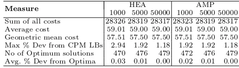
Table 3. Statistics on the results derived by AILS and ReVNS on the J30 benchmark set
Measure AILS ReVNS
1000 5000 50000 1000 5000 50000 Sum of all costs 28334 28319 28317 28326 28319 28317 Average cost 59.03 59.00 59.00 59.01 59.00 59.00 Geometric mean cost 57.52 57.50 57.50 57.51 57.50 57.50 Max % Dev from CPM LBs 2.94 1.92 1.18 2.94 1.92 1.18 No of Optimum solutions 463 476 479 470 476 479 Avg. % Dev from Optima 0.05 0.01 0.00 0.03 0.01 0.00
Table 4. Statistics on the results derived by AILS and ReVNS on the J60 benchmark set
Measure AILS ReVNS
1000 5000 50000 1000 5000 50000 Sum of all costs 38635 38521 38483 38679 38551 38477 Average cost 80.49 80.25 80.17 80.58 80.32 80.16 Geometric mean cost 78.65 78.47 78.41 78.72 78.53 78.42 Max % Dev from CPM LBs 110.39 105.20 103.90 106.49 105.20 102.60 No of Optimum solutions 295 295 295 295 295 295 Avg. % Dev from CPM LBs 11.35 11.10 10.91 11.47 11.10 10.88
Table 5. Statistics on the results derived by AILS and ReVNS on the J120 benchmark set
Measure AILS ReVNS
1000 5000 50000 1000 5000 50000 Sum of all costs 76256 75773 75279 76476 75686 75038 Average cost 127.09 126.29 125.47 127.46 126.14 125.06 Geometric mean cost 120.83 120.17 119.52 121.20 120.10 119.21 Max % Dev from CPM LBs 209.9 208.08 203.03 203.96 203.03 200.00 No of Optimum solutions 144 162 168 150 160 170 Avg. % Dev from CPM LBs 34.38 32.67 32.66 34.74 33.36 32.21
To compare AILS and ReVNS separately, we derived different statistical measures shown below in the Tables 3, 4 and 5. ReVNS is in general better than AILS in J30 and J60 benchmark sets, and this difference becomes larger when it comes to the large problem instances of the benchmark set J120, under the limit of 50000 schedules. More specifically, ReVNS achieves a better sum of all costs by 241 units, a better average cost by 0.41, a better geometric mean cost by 0.31, a better maximum % deviation from the CPM LBs by 3.03, it produces two more optimum solutions than AILS, and a better average % deviation from the CPM LBs by 0.45.
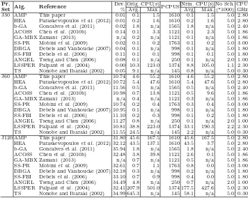
[image:16.595.178.416.292.360.2] [image:16.595.171.422.399.467.2] [image:16.595.174.423.506.573.2]Table 6. Comparisons to the-state-of-the-art algorithms on benchmarks sets J30, J60, and J120.
Pr.
Algorithm RS Reference % Dev.
Set 1000 5000 50000
J30 AMP EL This paper 0.02 0.01 0.00
ReVNS EL This paper 0.03 0.01 0.00
HEA EL Paraskevopouloset al.(2012) 0.03 0.01 0.00 AILS EL Paraskevopouloset al.(2012) 0.05 0.01 0.00
GA-MBX AL Zamani (2013) n/a n/a 0.00
SS-PR AL Mobiniet al.(2009) 0.05 0.02 0.01 b-GA RK Goncalves et al. (2011) 0.32 0.02 0.01 GA. TS-PR AL Kochetov and Stolyar (2003) 0.10 0.04 0.00 GAPS RK Mendeset al.(2009) 0.06 0.02 0.01 ACOSS AL Chenet al.(2010b) 0.14 0.06 0.01 SS-FBI RK Debelset al.(2006) 0.27 0.11 0.01 GA TO-RK Debels and Vanhoucke (2007) 0.15 0.04 0.02 GA-hybrid FBI AL Vallset al.(2008) 0.27 0.06 0.02 NG (FBI) AL Agarwalet al.(2011) 0.13 0.10 n/a
jPSO AL Chen (2011) 0.29 0.14 0.03
TS AL Nonobe and Ibaraki (2002) 0.46 0.16 0.05
GA AL Hartmann (2002) 0.38 0.22 0.08
ANGEL AL Tseng and Chen (2006) 0.22 0.09 n/a J60 HEA EL Paraskevopouloset al.(2012) 11.05 10.72 10.54 b-GA RK Goncalves et al. (2011) n/a 11.56 10.57 SS-PR AL Mobiniet al.(2009) 11.12 10.74 10.57
AMP EL This paper 11.09 10.74 10.65
GA-MBX AL Zamani (2013) n/a n/a 10.65
GAPS RK Mendeset al.(2009) 11.72 11.04 10.67 ACOSS AL Chenet al.(2010b) 11.72 11.04 10.67 GA TO-RK Debels and Vanhoucke (2007) 11.45 10.95 10.68 SS-FBI RK Debelset al.(2006) 11.73 11.10 10.71 GA-hybrid FBI AL Vallset al.(2008) 11.56 11.10 10.73 GA. TS-PR AL Kochetov and Stolyar (2003) 12.21 11.27 10.74
ReVNS EL This paper 11.47 11.10 10.88
AILS EL Paraskevopoulos et al (2012) 11.34 11.10 10.91 NG (FBI) AL Agarwalet al.(2011) 11.51 11.29 n/a
jPSO AL Chen (2011) 12.03 11.43 11.00
GA AL Hartmann (2002) 12.21 11.70 11.21 ANGEL AL Tseng and Chen (2006) 11.94 11.27 n/a TS AL Nonobe and Ibaraki (2002) 12.97 12.18 11.58 J120 ACOSS AL Chenet al.(2010b) 35.19 32.48 30.56 HEA EL Paraskevopouloset al.(2012) 33.32 32.12 30.78 GA TO-RK Debels and Vanhoucke (2007) 34.19 32.34 30.82
AMP EL This paper 33.08 31.80 30.88
GA-hybrid FBI AL Vallset al.(2008) 34.07 32.54 31.24
GA-MBX AL Zamani (2013) n/a n/a 31.30
SS-PR AL Mobiniet al.(2009) 34.49 32.61 31.37 GAPS RK Mendeset al.(2009) 35.87 33.03 31.44 SS-FBI RK Debelset al.(2006) 35.22 33.10 31.57 GA. TS-PR AL Kochetov and Stolyar (2003) 34.74 33.36 32.06
ReVNS EL This paper 34.74 33.36 32.21
AILS EL Paraskevopoulos et al (2012) 34.38 32.67 32.66 b-GA RK Goncalves et al. (2011) n/a 35.94 32.76
jPSO AL Chen (2011) 35.71 33.88 32.89
NG (FBI) AL Agarwalet al.(2011) 34.65 34.15 n/a GA AL Hartmann (2002) 37.19 35.39 33.21 ANGEL AL Tseng and Chen (2006) 36.39 34.49 n/a TS AL Nonobe and Ibaraki (2002) 40.86 37.88 35.85
4.3.2 Performance of the AMP
Having tested the proposed improvement method’s performance, the comparative analysis proceeds by evaluating AMP’s performance. Table 6 reports the results of metaheuristic methodologies of the literature on J30, J60 and J120 problem sets. The table has an identical structure to Table 2. The second column presents the abbreviations of the solution methodologies as originally named by the authors (ACOSS – Ant Colony Optimization Scatter Search, PR–Path Relinking, GAPS– Genetic Algorithm for Project Scheduling, GA-MBX–Genetic Algorithm Magnet-based Crossover, b-GA–biased Genetic Algorithm, FBI–Forward Backward Improvement, ANGEL–ANt colony op-timization GEnetic algorithm Local search, NG–NeuroGenetic). The next column give the repre-sentation scheme, e.g., TO-RK for the Topological Order Random Key reprerepre-sentation, while the next column gives the references. Lastly, the multicolumn presents the % deviations as described in Table 2. The order of the papers is in accordance to the algorithmic performances under 50000 schedules, for each different benchmark set.
[image:17.595.160.438.64.507.2]explic-itly calculated due to the decomposition phase of the algorithm. Nevertheless, the authors report DGBA’s computational times, thus included in the Tables 10 and 11.
AMP achieves 0,02%,0,01% and 0,00% average deviation from the optimum solutions of the J30 set at 1000, 5000 and 50000 schedules, respectively. Regarding the J60 set, AMP obtains 11,09 %, 10,74 and % 10,65 % average deviation from the CPM lower bounds. On the large scale benchmark set J120, our AMP outperforms all the solution approaches when 1000 and 5000 schedules are examined, presenting 33.08 % and 31.80 % deviations from the CPM lower bounds. The latter results improve the current best results presented by Paraskevopoulos et al. (2012) by 0.24% and 0.32%. When 50000 schedules are examined, AMP remains competitive presenting 30.88 % deviation from the CPM lower bounds. Lastly, it is worth mentioning that, ReVNS holds a good ranking in the list of Table 6, justifying his role as an improvement method. Nevertheless, the AMP framework is by far better than the ReVNS, improving by 1.66%, 1.56% and 1.33% the results produced by ReVNS for 1000, 5000 and 50000 schedules respectively, highlighting the effectiveness of AMP and its impact on the solution quality.
To compare HEA and AMP separately, we present different statistical measures in Tables 7, 8 and 9. One could observe that AMP’s performance is very competitive compared to HEA’s. AMP’s main strength is to produce very good results in fewer schedules examined, as clearly shown in Table 6. More specifically, regarding the 5000 schedules examined, AMP achieves a better sum of all costs by 179 units, a better average cost by 0.3, a better geometric mean cost by 0.24, it produces 4 more optimum solutions than HEA and it lastly achieves a better average % deviation from the CPM LBs by 0.32. AMP performs also better than HEA under the limitation of 1000 schedules. Specifically, AMP achieves a better sum of all costs by 137 units, a better average cost by 0.23, a better geometric mean cost by 0.2, a better maximum % deviation from the CPM LBs by 4.04, it produces 6 more optimum solutions than HEA and it lastly achieves a better average % deviation from the CPM LBs by 0.24.
Table 7. Statistics on the results derived by HEA and AMP on the J30 benchmark set
Measure 1000 HEA5000 50000 1000AMP5000 50000
Sum of all costs 28326 28319 28317 28323 28319 28317 Average cost 59.01 59.00 59.00 59.01 59.00 59.00 Geometric mean cost 57.51 57.50 57.50 57.51 57.50 57.50 Max % Dev from CPM LBs 2.94 1.92 1.18 1.92 1.92 1.18 No of Optimum solutions 470 476 479 472 476 479 Avg. % Dev from Optima 0.03 0.01 0.00 0.02 0.01 0.00
Table 8. Statistics on the results derived by HEA and AMP on the J60 benchmark set
Measure HEA AMP
1000 5000 50000 1000 5000 50000 Sum of all costs 38532 38425 38361 38539 38420 38389 Average cost 80.28 80.05 79.92 80.07 80.32 80.01 Geometric mean cost 78.48 78.31 78.22 78.51 78.32 78.27 Max % Dev from CPM LBs 106.49 103.9 101.3 105.2 101.3 101.3 No of Optimum solutions 297 297 297 297 297 297 Avg. % Dev from CPM LBs 11.05 10.72 10.54 11.09 10.74 10.65
Table 9. Statistics on the results derived by HEA and AMP on the J120 benchmark set
Measure HEA AMP
[image:18.595.179.415.402.470.2] [image:18.595.181.416.521.589.2] [image:18.595.173.423.639.707.2]4.3.3 Comparisons on the computational times
In this section the computational times are reported. There are papers that report running times that are linked to 5000 (and lower) schedules, while other report more than 50000 schedules or they do not mention the number of schedules, all included in Tables 10 and 11.
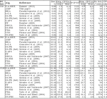
Table 10. Computational times for up to 5000 schedules examined
Pr.
Alg. Reference Dev. Orig. CPU(s)PCPUSNrm. CPU(s) No Sch. CPU
Set % Avg. Max. Avg Max. (*1000) GHz
J30 AMP This paper 0.01 0.1 1.5 1610 0.1 1.5 5.0 2.80
HEA Paraskevopouloset al.(2012) 0.01 0.2 1.6 1610 0.2 1.6 5.0 2.80 b-GA Goncalves et al. (2011) 0.02 1.8 n/a 1565 1.8 n/a 5.0 2.40 ACOSS Chenet al.(2010b) 0.14 0.1 3.3 1121 0.1 2.3 5.0 1.86 GA-MBX Zamani (2013) n/a 0.2 n/a 1121 0.1 n/a 5.0 1.86 SS-PR Mobiniet al.(2009) 0.02 0.1 0.2 1763 0.1 0.2 5.0 3.00 DBGA Debels and Vanhoucke (2007) 0.04 0.1 n/a 998 0.1 n/a 5.0 1.80 SS-FBI Debelset al.(2006) 0.11 0.1 0.1 998 0.1 0.1 5.0 1.80 ANGEL Tseng and Chen (2006) 0.08 0.1 n/a 250 0.1 n/a 2.0 1.00 LSSPER Palpantet al.(2004) 0.00 10.3 123.0 1374 8.8 105.0 1.1 2.30 TS Nonobe and Ibaraki (2002) 0.05 9.1 n/a 145 0.8 n/a 5.0 0.30 J60 AMP This paper 10.74 4.6 55.2 1610 4.6 55.2 5.0 2.80 HEA Paraskevopouloset al.(2012) 10.72 5.4 47.6 1610 5.4 47.6 5.0 2.80 b-GA Goncalves et al. (2011) 11.56 0.5 n/a 1565 0.5 n/a 5.0 2.40 ACOSS Chenet al.(2010b) 10.98 0.7 13.8 1121 0.5 9.6 5.0 1.86 GA-MBX Zamani (2013) n/a 0.4 n/a 1121 0.3 n/a 5.0 1.86 SS-PR Mobiniet al.(2009) 10.74 0.2 0.4 1763 0.3 0.4 5.0 3.00 DBGA Debels and Vanhoucke (2007) 10.95 0.1 n/a 998 0.1 n/a 5.0 1.80 SS-FBI Debelset al.(2006) 11.10 0.2 0.3 998 0.1 0.2 5.0 1.80 ANGEL Tseng and Chen (2006) 11.27 0.8 n/a 250 0.1 n/a 2.0 1.00 LSSPER Palpantet al.(2004) 10.81 38.8 223.0 1374 33.1 190.3 2.2 2.30 TS Nonobe and Ibaraki (2002) 11.55 24.5 n/a 145 2.2 n/a 5.0 0.30 J120 AMP This paper 31.80 45.6 167.5 1610 45.6 167.5 5.0 2.80 HEA Paraskevopouloset al.(2012) 32.12 43.5 137.1 1610 43.5 3.7 5.0 2.80 b-GA Goncalves et al. (2011) 35.94 1.8 n/a 1565 1.8 n/a 5.0 2.40 ACOSS Chenet al.(2010b) 32.48 3.8 39.8 1121 2.6 0.1 5.0 1.86 GA-MBX Zamani (2013) n/a 0.7 n/a 1121 0.5 n/a 5.0 1.86 SS-PR Mobiniet al.(2009) 32.61 0.7 1.1 1763 0.8 0.0 5.0 3.00 DBGA Debels and Vanhoucke (2007) 32.18 0.3 n/a 998 0.2 n/a 5.0 1.80 SS-FBI Debelset al.(2006) 33.10 0.7 0.9 998 0.4 0.0 5.0 1.80 ANGEL Tseng and Chen (2006) 34.49 4.8 n/a 250 0.7 n/a 2.0 1.00 LSSPER Palpantet al.(2004) 32.41 207.9 501.0 1374 177.5 427.6 5.0 2.30 TS Nonobe and Ibaraki (2002) 34.99 645.3 n/a 145 58.1 n/a 5.0 0.30
To be able to normalise the computational times according to the different computational power used, we used the performance lists of http://www.cpubenchmark.net/. All the comparisons were made according to the Passmark CPU Score (PCPUS). As we were unable to find PCPUS for Sun and AMD 400 MHz systems on http://www.cpubenchmark.net/, we used an Intel equivalent. Every computational time was normalised by using AMP as the reference point, e.g., Nrm. CPU(Alg)= PCPUS(Alg)Orig.CPU(Alg)/PCPUS(AMP).
Tables 10 and 11 report the papers sorted according to the date of publication. The four first columns are common with the previous tables , while the fifth and the sixth column present the average and the maximum CPU time in seconds, respectively, as reported by the original authors. Note that the abbreviation LSSPER stands for Local Search with SubProblem Exact Resolution, PBA stands for Population based approach and FF stands for Filter and Fan. The seventh column reports the score of PCPUS, and using that, columns eight and nine report the normalised running times. The number of schedules and the processor’s frequency is reported on the tenth and eleven columns, respectively. This is not sufficient though for determining the effectiveness of the solution approaches, since the computer architecture and operating systems must also be thoroughly investigated. Tables 10 and 11 indicate that the running times of AMP are reasonable, illustrating its effectiveness in solving large scale RCPSPs.
5. Conclusions and Further Research
[image:19.595.120.476.131.418.2]Table 11. Computational times for 50000 (and more) schedules examined.
Pr.
Alg. Reference Dev. Orig. CPU(s)PCPUSNrm. CPU(s) No Sch. CPU
Set % Avg. Max. Avg Max. (*1000) GHz.
J30 GA-MBX Zamani (2013) 0.00 1.3 n/a 1121 0.9 n/a 50 1.86
AMP This paper 0.00 0.2 3.7 1610 0.2 3.7 50 2.80
HEA Paraskevopouloset al.(2012) 0.00 0.2 2.9 1610 0.2 2.9 50 2.80 b-GA Goncalves et al. (2011) 0.01 18.0 n/a 1565 17.4 n/a 50 2.40 SS-PR Mobiniet al.(2009) 0.01 0.8 1.4 1763 0.9 1.5 50 3.00 SS-PR(fast) Mobiniet al.(2009) 0.02 0.7 1.4 1763 0.7 1.5 n/a 3.00 GAPS Mendeset al.(2009) 0.01 5.0 n/a 340 1.1 n/a 50 1.33
FF Ranjbar (2008) 0.00 5.0 5.0 1763 5.5 5.5 n/a 3.00
DBGA Debels and Vanhoucke (2007) 0.02 0.5 n/a 998 0.3 n/a 50 1.80 SS-FBI Debelset al.(2006) 0.01 0.7 1.3 998 0.4 0.8 50 1.80 PBA Vallset al.(2004) 0.10 1.2 5.5 145 0.1 0.5 n/a 0.40 VNS Fleszar and Hindi (2004) 0.01 0.6 5.9 250 0.1 0.9 n/a 1.00 TS-FBI Vallset al.(2003) 0.06 1.6 6.2 145 0.1 0.6 n/a 0.40 J60 GA-MBX Zamani (2013) 10.65 2.8 n/a 1121 2.0 n/a 50 1.86 AMP This paper 10.65 15.3 93.8 1610 15.3 93.8 50 2.80 HEA Paraskevopouloset al.(2012) 10.54 16.3 89.2 1610 16.3 89.2 50 2.80 b-GA Goncalves et al. (2011) 10.57 5.3 n/a 1565 5.2 n/a 50 2.40 SS-PR Mobiniet al.(2009) 10.57 2.0 3.0 1763 2.2 3.3 50 3.00 SS-PR (fast) Mobiniet al.(2009) 10.91 1.1 n/a 1763 1.2 n/a n/a 3.00 GAPS Mendeset al.(2009) 10.67 20.1 n/a 340 4.2 n/a 50 1.33 FF Ranjbar (2008) 10.56 5.0 5.0 1763 5.5 5.5 n/a 3.00 DBGA Debels and Vanhoucke (2007) 10.68 1.1 n/a 998 0.7 n/a 50 1.80 SS-FBI Debelset al.(2006) 10.71 1.9 2.6 998 1.2 1.6 50 1.80 PBA Vallset al.(2004) 10.89 3.7 22.6 145 0.3 2.0 n/a 0.40 VNS Fleszar and Hindi (2004) 10.94 8.9 80.7 250 1.4 12.5 1653 1.00 TS-FBI Vallset al.(2003) 11.12 2.8 14.6 145 0.2 1.3 n/a 0.40 J120 GA-MBX Zamani (2013) 31.30 5.8 n/a 1121 4.0 n/a 50 1.86 AMP This paper 30.88 118.5 601.0 1610 118.5 601.0 50 2.80 HEA Paraskevopouloset al.(2012) 30.78 123.5 551.0 1610 123.5 551.0 50 2.80 b-GA Goncalves et al. (2011) 32.76 18.0 n/a 1565 17.4 n/a 50 2.40 SS-PR Mobiniet al.(2009) 31.37 7.1 10.1 1763 7.7 11.1 50 3.00 SS-PR (fast) Mobiniet al.(2009) 32.27 6.2 n/a 1763 6.7 n/a n/a 3.00 GAPS Mendeset al.(2009) 31.44 112.5 n/a 340 23.7 n/a 50 1.33 FF Ranjbar (2008) 31.42 5.0 5.0 1763 5.5 5.5 n/a 3.00 DBGA Debels and Vanhoucke (2007) 30.69 3.0 n/a 998 1.9 n/a 50 1.80 SS-FBI Debelset al.(2006) 31.57 6.7 9.2 998 4.1 5.7 50 1.80 PBA Vallset al.(2004) 31.58 59.4 264.0 145 5.4 23.8 n/a 0.40 VNS Fleszar and Hindi (2004) 33.10 219.9 1127.0 250 34.1 175.0 10778 1.00 TS-FBI Vallset al.(2003) 34.53 17.0 43.9 145 1.5 4.0 n/a 0.40
into the solution space, while using a ReVNS as an improvement method. The proposed ReVNS conducts a thorough exploration of the solution neighbourhood and consorts with a perturbation strategy to escape from local optima.
The main goal of this paper was to prove whether the AMP framework, which is quite successful in solving hard combinatorial optimisation problems, is suitable for solving large scale RCPSPs. Computational experiments on well known RCPSP instances showed that AMP produces con-sistently high quality solutions for all data sets and performance criteria. In particular, AMP outperforms all solution methodologies for large scale RCPSPs under the termination criteria of 1000 and 5000 schedules, while remaining highly competitive when the 50000 schedules are used as a termination criterion. It is worth mentioning also that, ReVNS, a major AMP component, presents a good performance justifying its role as an improvement method.
Challenging the proposed adaptive memory strategies for capturing elite solution elements of other important variants of the classical RCPSP, e.g., multiple modes and/or multiple projects, is a worth pursuing research avenue.
Acknowledgements
[image:20.595.116.478.56.389.2]References
Agarwal A., S. Colak, and S. Erenguc, 2011. “A neurogenetic approach for the resource-constrained project scheduling problem”,Computers & Operations Research, 38, 44–50.
Artigues C., P. Michelon, and S. Reusser, 2003. “Insertion techniques for static and dynamic resource-constrained project scheduling”,European J. of Operational Research, 149, 249–267.
Blazewicz J., J.K. Lenstra, and A.H.G. Rinnooy Kan, 1983. “Scheduling Subject to Resource constraints: Classification and Complexity”,Discrete Applied Mathematics, 5, 11–24.
Bouleimen K. and H. Lecocq, 2003. “A new efficient simulated annealing algorithm for the resource-constrained project scheduling problem and its multiple modes version”, European J. of Operational Research, 149, 268–281.
Brucker P., S. Knust, A. Schoo, and O. Thiele, 1998.“A branch and bound algorithm for the resource-constrained project scheduling problem”,European J. of Operational Research, 107(2), 272–288.
Cardona-Valds Y., A. lvarez, J. Pacheco, 2014. “Metaheuristic procedure for a bi-objective supply chain design problem with uncertainty”.Transportation Research Part B, 60, 66-84.
Chen R.M., C.L. Wub, C.M. Wang, and S.T. Lo, 2010a.“Using novel particle swarm optimization scheme to solve resource-constrained scheduling problem in PSPLIB”,Expert Systems with Applications, 37, 1899– 1910.
Chen W., Y.J. Shi, H.F. Teng, X.P. Lan, and L.C. Hu, 2010b. “An efficient hybrid algorithm for resource-constrained project scheduling”,Information Sciences, 180, 1031–1039.
Chen R.M. 2011.“Particle swarm optimization with justification and designed mechanisms for resource-constrained project scheduling problem”,Expert Systems with Applications, 38, 7102–7111.
Czogalla J. and A. Finik, 2009.“Fitness Landscape Analysis for the Resource Constrained Project Scheduling Problem”,LNCS, 5851, 104–118.
Debels D., B. Reyck, R. Leus, and M. Vanhoucke, 2006. “A hybrid scatter search/electromagnetism meta heuristic for project scheduling”,European J. of Operational Research, 169, 638–653.
Debels D. and M. Vanhoucke, 2007.“A decomposition-based genetic algorithm for the resource constrained project scheduling problem”,Operations Research, 55, 457–469.
Demassey S., C. Artigues, and P. Michelon, 2005.“Constraint-Propagation-Based Cutting Planes: An Ap-plication to the Resource-Constrained Project Scheduling Problem ”,INFORMS J. on Computing, 17(1), 52–65.
Fleszar K. and K. Hindi, 2004.“Solving the resource-constrained project scheduling problem by a variable neighborhood search”,European J. of Operational Research, 155, 402–413.
Fleurent C. and F. Glover, 1999. “Improved Constructive Multistart Strategies for the Quadratic Assignment Problem Using Adaptive Memory”,INFORMS J. on Computing, 11(2), 198–204.
Garey M. and D. Johnson. 1979.“Computers and intractability: A guide to the theory of NP-completeness”, New York: W.H. Free man and Company.
Glover, F. 1997.“Tabu search and adaptive memory programming - advances, applications and challenges”. Barr RS, Helgason RV, Kennington JL, eds., Interfaces in Computer Science and Operation Research: Advances in Metaheuristics. (Kluwer, Boston MA, US), 1–75.
Glover F. G.A. Kochenberger and B. Alidaee, 1998. “Adaptive Memory Tabu Search for Binary Quadratic Programs”,Management Science, 44(3), 336–345.
Goncalves J.F., M.G.C. Resende, and J.J.M. Mendes, 2011.“A biased random-key genetic algorithm with forward-backward improvement for the resource constrained project scheduling problem”,J. of Heuristics, 17, 467-486.
Gounaris E.C., P.P. Repoussis, C.D. Tarantilis, W. Wiesemann, and C.A. Floudas, 2014.“An Adaptive Memory Programming framework for the Robust Capacitated Vehicle Routing Problem”.Transportation Science, http://dx.doi.org/10.1287/trsc.2014.0559.
Hartmann S. and D. Briskorn, 2010. “A survey of variants and extensions of the resource-constrained project scheduling problem”European J. of Operational Research, 207, 1–14.
Hartmann S. 2002. “A self-adapting genetic algorithm for project scheduling under resource constraints”,
Naval Research Logistics, 49, 433–448.
Kochetov Y. and A. Stolyar, 2003. “Evolutionary local search with variable neighbourhood for the resource constrained project scheduling problem”, InProceedings of the Third International Workshop of Computer Science and Information Technologies, Russia.