Geometrically designed, variable knot regression splines

City, University of London Institutional Repository

Citation

: Kaishev, V. K., Dimitrova, D. S., Haberman, S. and Verrall, R. J. (2016).

This is the accepted version of the paper.

This version of the publication may differ from the final published

version.

Permanent repository link:

Link to published version

: http://dx.doi.org/10.1007/s00180-015-0621-7

Copyright and reuse:

City Research Online aims to make research

outputs of City, University of London available to a wider audience.

Copyright and Moral Rights remain with the author(s) and/or copyright

holders. URLs from City Research Online may be freely distributed and

linked to.

City Research Online: http://openaccess.city.ac.uk/ [email protected]

Online supplement to: Geometrically designed, variable knot

regression splines

Vladimir K. Kaishev∗, Dimitrina S. Dimitrova, Steven Haberman and Richard Verrall

Cass Business School, City University London

In this supplement, we first present simulation results related to sections 3.1 and 4.1 of the

paper and second, we present further test results with the purpose of thoroughly testing the

numerical performance of the GeDS method and its properties, established in section 3.

1

Simulation results supplementing sections 3.1 and 4.1.

1.1 Simulation results supplementing section 3.1

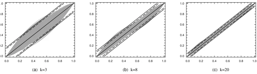
In order to illustrate the bound (25) and how accurately the averaging knot location (20) solves

system (19) with respect to the knots for given Greville sites, we have randomly generated

abscissa values ξj, j = 1, . . . , p for three fixed numbers of vertices p, equal respectively to 6

(k = 3), 11 (k = 8) and 23 (k = 20). The number of simulations for each value of p is 1000.

The corresponding thousand graphs of∑p_i=1ξiNi,n(t), t∈[0,1], in the quadratic case (n= 3),

with knots defined by (20) , are plotted in Figure 1 (a), (b) and (c).

In Figure 1, two corridors are also shown. The first, defined by the dashed lines, is based

on the 95 sample percentile of e=∥t−∑p_i=1ξiNi,3(t)∥, denoted by ˆe0.95. The second corridor

(the solid lines) is based on the 95 sample percentile ˆε0.95 of the bound in (25), denoted by

ε. As can be seen from Figure 1, the maximum deviation of ∑p_i=1ξiNi,3(t) from the straight

line t is reasonable, and rapidly decreases as the number of knots increases. Thus, the higher

the number of knots, the more accurately the averaging knot location (20) solves system (19).

Similar conclusions are found to hold for the cubic case (n= 4), applying both ˆe0.95 and ˆε0.95.

As seen from Figure 1, the solid line deviates insignificantly from the dashed line, so that the

bound in (25) is nearly sharp for n= 3.

∗_{Corresponding author’s address: Faculty of Actuarial Science and Insurance, Cass Business School, City}

0.0 0.2 0.4 0.6 0.8 1.0 0.0

0.2 0.4 0.6 0.8 1.0

HaL k=3

0.0 0.2 0.4 0.6 0.8 1.0 0.0

0.2 0.4 0.6 0.8 1.0

HbL k=8

0.0 0.2 0.4 0.6 0.8 1.0 0.0

0.2 0.4 0.6 0.8 1.0

HcL k=20

Figure 1: Graphs of 1000 simulations of∑p_i=1ξiNi,3(t), with¯tk,3according to (20) and estimates

of ˆe0.95and ˆε0.95for: (a)p= 6 (k= 3), ˆe0.95= 0.17, ˆε0.95= 0.18; (b)p= 11 (k= 8), ˆe0.95= 0.10,

ˆ

ε0.95= 0.12; (c)p= 23 (k= 20), ˆe0.95= 0.05, ˆε0.95= 0.07.

Remark 1.1 Note that, as seen from the bound, (25) the quality of the reconstruction of

ˆ

f(δl,2,αˆ;x) in stage B, using eitherC_f(˜_{tl−(n−2),n,αˆ;x)} orC_f(¯_{tl−(n−2),n,αˆ;x)}, depends on the

max-imal distance between the knots δl,2, obtained in stage A. By adding more knots at appropriate

sites, the maximal distance may be decreased, which will make the bound (25) sharper.

How-ever, such an addition should be done in a way that preserves the geometry offˆ(δl,2,αˆ;x). To

achieve the latter, one may apply the Boehm’s knot insertion formula (see e.g., Farin 2002)and

add a knot at the middle of the interval, where max_{j∈{1,...,p−1}}(ξj+1 −ξj) is attained. It is

worth pointing out though that based on our experience with GeDS, the reconstruction in stage

B achieved using (20) is quite satisfactory and such knot insertion has not been implemented.

Remark 1.2 The choice of the knots ¯tl−(n−2),n in (20) can also be given an interpretation,

related to the problem of optimal recovery of a function g, by interpolating it at some fixed

points, with an n-th order spline on a set of knots tk,n. The problem is to find the optimal

set of knots, topt_k,n for which the bound on the interpolation error is minimized over all possible choices of tk,n. Such optimal interpolation has been considered by Micchelli et al. (1976). An

approximate solution to this optimal recovery problem has been proposed by De Boor (2001).

In our case, if we apply this scheme to the polygon fˆ(δl,2,αˆ;x) and view its vertices (ξi,αˆi)

as given data points, then the approximate solution of this optimal interpolation problem, as

2 3 4 5 6 7 8 9 10 11 12 13 14 15 N=180 , SNR=7 N=90 , SNR=7 N=180 , SNR=5

0 100 200 300 400 500

Linear

Quadratic _Cubic

10-2

10-3

10-4

10-5

HbLΑ=0.9 ,Β=0.7

2 3 4 5 6 7 8 9 10 11 12 13 14 15 N=180 , SNR=7 N=90 , SNR=7 N=180 , SNR=5

0 100 200 300 400 500

Linear

Quadratic Cubic

10-2

10-3

10-4

10-5

HcLΑ=0.9 ,Β=0.5

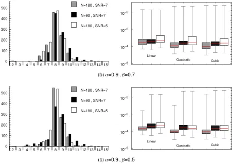
Figure 2: Frequency plots of the number of knots, l, (left panels) and box plots of the MSE values (right panels) of the 1000 linear GeD spline fits for: (b) and (c) - three different choices (combinations) of number of data, N, and SNR, obtained with α_{exit = 0}.9, and β = 0.7 and

1.2 Simulation results supplementing section 4.1

Using the test example from section 4.1 of the paper, the performance of GeDS is also tested

when the number of simulated data points increases from N = 90 to N = 180, and when the

SNR worsens from SNR=7 to SNR=5 approximately. The latter is achieved by increasing the

noise level toU[−0.065,0.065]. Thus, on panels (b) and (c) of Figure 2, the results from Figure

4 (b) and (c) in the paper , obtained withα_{exit = 0}.9 (illustrated in black), are compared with

the results from the GeDS method applied to twice as many data points (N = 180) with the

same level of noise (SNR=7), or a higher noise level, SNR=5. As expected, the MSE values

improve for both β = 0.7 and β = 0.5 when more data are used with the latter leading to

slightly better figures, see the gray boxes on Figure 2 (b) and (c) respectively. Furthermore,

the results worsen when the noise level increases, again with β = 0.5 providing slightly better

MSE values, see the white boxes on Figure 2 (b) and (c) respectively.

2

Further numerical examples

Here we present further test results on various simulated examples (see Examples 1-6 as specified

in Table 1), used in many other studies on variable knot spline methods (cf. Fan and Gijbels

1995, Donoho and Johnstone 1994, Luo and Wahba 1997, Lee 2000, 2002a,b,c, Zhou and Shen

2001, and Pittman 2002). We have illustrated the impact on the GeDS knot location and

related mean square error (MSE), of different assumptions and choices made in constructing

the GeDS estimate, namely, different levels of the signal-to-noise ratio (SNR from 2 to 7),

sample sizes (N =150, 256, 512, 2048) and levels of smoothness of the underlying function

(smooth, medium smooth and wiggly functions), different choices of the parametersα_{exit and}β

(α_{exit = 0}.8,0.9,0.95,0.99,0.995,0.999,β = 0.3,0.5,0.7), different choice of the model selection

criterion (GeDS criterion, GCV and SURE), and different degree of the GeD spline estimate

(linear, quadratic and cubic). We have also compared the GeDS knot selection strategy with

the results from the above mentioned established approaches and equally spaced knots.

As discussed in the paper, in order to obtain a GeD spline fit, most often it is necessary to

input only the set of data {xi, yi}Ni=1 and use the default values of the GeDS model selection

parameters α_{exit = 0}.9, β = 0.5. The latter, as illustrated by the examples given below,

values of the parameters can be appropriately refined depending on the level of the

signal-to-noise ratio and on the degree of smoothness/wiggliness of f. As can be concluded from the

numerical tests performed here and based on our extensive experience with GeDS, when the

SNR is high and f is smooth, see e.g. the simulated example presented in section 4.1 of the

paper, recommended values are β ∈[0.5,0.7], α_exit ∈[0.9,0.95]. If the SNR is high and f is

a wiggly function, as in Examples 3-6 below, then the recommended choice is β ∈ [0.5,0.7],

α_exit ∈[0.99,0.995], since otherwise underfitting may result. In the case when SNR is low and

f is smooth, see e.g. Examples 1-2, one may use β ∈[0.3,0.5], α_exit∈[0.9,0.95]. Finally, it is

known that when the SNR is low and the underlying function is very unsmooth recoveringf is

very difficult and different choices ofβ andα_{exit may need to be attempted. But our experience}

shows that in the majority of cases choices of α_exit ∈ (0,0.8) generally lead to underfitting,

especially for less smooth functions, and thus, should be avoided, as well as valuesβ /∈[0.3,0.7]

which put too high/low weight on the cluster range as opposed to the mean residual value

within each cluster of residuals of same sign (see Appendix A of the paper).

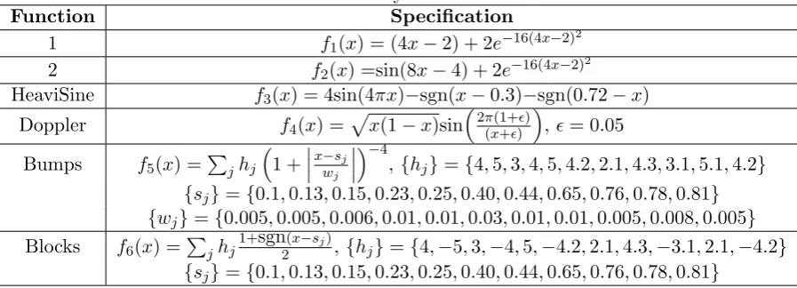
Table 1: Summary of test functions.

Function Specification

1 f1(x) = (4x−2) + 2e−16(4x−2)

2

2 f2(x) =sin(8x−4) + 2e−16(4x−2)

2

HeaviSine f3(x) = 4sin(4πx)−sgn(x−0.3)−sgn(0.72−x)

Doppler f4(x) =

√

x(1−x)sin

(

2π(1+ϵ) (x+ϵ)

)

,ϵ= 0.05

Bumps f5(x) =

∑

jhj

(

1 +x−sj

wj

)−4,{hj}={4,5,3,4,5,4.2,2.1,4.3,3.1,5.1,4.2}

{sj}={0.1,0.13,0.15,0.23,0.25,0.40,0.44,0.65,0.76,0.78,0.81}

{wj}={0.005,0.005,0.006,0.01,0.01,0.03,0.01,0.01,0.005,0.008,0.005} Blocks f6(x) =

∑

jhj1+sgn₂(x−sj),{hj}={4,−5,3,−4,5,−4.2,2.1,4.3,−3.1,2.1,−4.2}

{sj}={0.1,0.13,0.15,0.23,0.25,0.40,0.44,0.65,0.76,0.78,0.81}

In order to investigate the performance of the GeD spline method and to facilitate

com-parison of GeDS with existing smoothing methods, we have simulated data using the functions

listed in Table 1, which have been widely utilized in testing other existing smoothing

proce-dures. The data sets, used to test GeDS were simulated by adding noise,ϵ∼ N(0, σ_ϵ2), to each

of the six functions, as given in Table 2. The proposed GeDS method has been implemented

usingM athematica9.0 and a standard PC (Intel core i7 CPU, 2.93 Ghz, 8GB RAM) has been

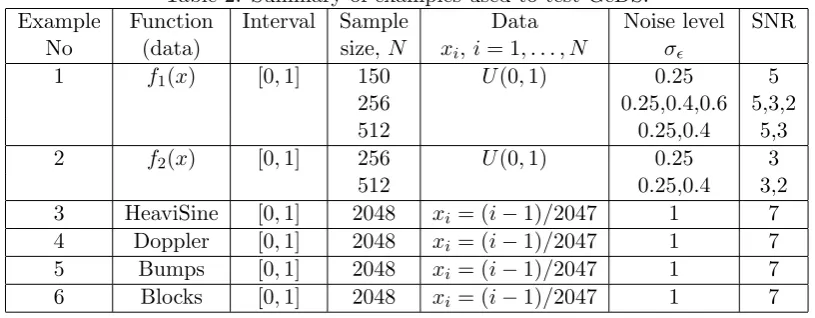
Table 2: Summary of examples used to test GeDS.

Example Function Interval Sample Data Noise level SNR

No (data) size,N xi,i= 1, . . . , N σϵ

1 f1(x) [0,1] 150 U(0,1) 0.25 5

256 0.25,0.4,0.6 5,3,2

512 0.25,0.4 5,3

2 f2(x) [0,1] 256 U(0,1) 0.25 3

512 0.25,0.4 3,2

3 HeaviSine [0,1] 2048 xi = (i−1)/2047 1 7

4 Doppler [0,1] 2048 xi = (i−1)/2047 1 7

5 Bumps [0,1] 2048 xi = (i−1)/2047 1 7

6 Blocks [0,1] 2048 xi = (i−1)/2047 1 7

As can be seen, we have included test examples with a wide range of values of SNR (from 2

to 7), and with various characteristics of the data set: small and large sample sizes (150, 256,

512 and 2048),x-values in a grid or uniformly generated within the interval [0,1]. Note also that

the test functions possess different smoothness properties: some of them are relatively smooth

(Examples 1-2), while others are very wiggly, with possible discontinuities (Examples 3-6).

In order to compare the quality of the fits produced by GeDS to those given by other authors,

we use the mean square error (MSE), defined with respect to the true function f, rather than

to the data, i.e.

MSE =

{ _N ∑

i=1

(

f(xi)−fˆ

(

¯_{tl−(n−2),n,θ}ˆ_;xi))2

}

/N.

Note that, in practice, the underlying function is unknown and a set of observations is fitted.

For this reason, we give also the L2-error of approximation, defined as the square root of the

residual sum of squares, i.e. √RSS. However, for a fair comparison between the smoothing

methods, one would need all model parameter values, such as the number of knots (regression

functions) and degree of the spline fits etc., which often are not reported in full. In order to

compare the speed of computation on equal grounds, one would need to implement all of the

available methods using the same hardware and software, and test them on entirely identical

simulated data sets. Such a comparison is outside the scope of this paper.

Based on the test examples, we illustrate the linear GeD spline fit produced at the end of

Stage A, and the quadratic and the cubic final GeD spline estimators resulting from Stage B.

We have run GeDS with 1000 simulated data sets for Examples 1 and 2, and 100 data sets for

Luo and Wahba 1997 who use 400 simulated data sets for Examples 1 and 2, and 31 data sets

for Examples 3-6; or Lee (2002a,b) who uses 50 simulated data sets for Examples 3-6). This

allows us to compute the median of the MSE, obtained using GeDS, and compare it with the

MSE medians given by other authors. In each example, we have plotted a single data set,

randomly chosen among the simulated data sets, with the obtained GeD spline fit and the true

underlying function, in order to visually illustrate the results.

We compare most of our results with those of Luo and Wahba (1997) since, along with

the median MSE values for their fits, they give also the order and the number of the basis

functions and with Lee (2002a,b) who thoroughly compares eight different smoothing methods

on Examples 3-6 and provides extensive box-and-whisker plots with the resulting log(M SE)

values as well as reports the median MSEs for all the methods. Note the difference in the scaling

of functions 3-6 used here and in Lee (2002a,b) which requires adjustment of the reported MSE

values as (M SE/512)∗const2). Also, the Bumps and Blocks of Luo and Wahba (1997) are

not directly comparable, since the authors use versions of these functions which differ from

ours, i.e. from those proposed by Donoho and Johnstone (1994). Furthermore, it should be

noted that based on the comparative study of the eight methods presented in Lee (2002a,b),

among which the MDL method proposed by the author, DMS of Denison et al. (1998), SK of

Smith and Kohn (1996) and RSW of Ruppert et al. (1995), it is shown that the proposed MDL

method is superior to the other smoothing methods when the target function is non-smooth.

So, for Examples 3-6 we compare the GeDS performance with the (minimum) median MSE

values reported by Lee (2002a,b) for the MDL method and the corresponding box-and-whisker

plots.

The GeD fits in Examples 1 and 2 are compared with the optimal spline fits, produced

following the standard LS non-linear optimization approach and its penalized version, developed

by Lindstrom (1999). The latter has been implemented, using the transformation of the knots,

proposed by Jupp (1978) and theMathematica functionNMinimize, which attempts to find the

global minimum. Due to the drawbacks of the non-linear optimization approach, it has not

been feasible to produce optimal spline fits for the spatially inhomogeneous functions, recovered

in Examples 3-6 from large data sets, usingMathematica, and a standard PC.

Example 1. This smooth function first appears as a test example in Fan and Gijbels (1995).

(2001) to test their fitting procedures. With this example, we illustrate the performance of

GeDS for data sets with different sample sizes, namely N = 150, N = 256 and N = 512, and

various noise levels, assuming ϵis normally distributed, namelyϵ∼N(0,0.252_{),ϵ∼N(0,0.4}2₎

and ϵ ∼ N(0,0.62), corresponding approximately to SNR=5, SNR=3 and SNR=2. It takes

between 0.90 seconds and 1.83 seconds to compute the GeDS fits, given in Table 3. The L2

-errors of all the fits are within the noise level and their visual quality is very good, as can be

seen from Figure 3.

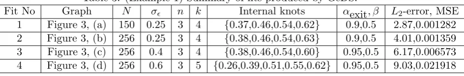
Table 3: (Example 1) Summary of fits produced by GeDS.

Fit No Graph N σϵ n k Internal knots α_exit, β L2-error, MSE

1 Figure 3, (a) 150 0.25 3 4 {0.37,0.46,0.54,0.62} 0.9,0.5 2.87,0.001282 2 Figure 3, (b) 256 0.25 3 4 {0.38,0.46,0.54,0.63} 0.9,0.5 4.01,0.001359 3 Figure 3, (c) 256 0.4 3 4 {0.38,0.46,0.54,0.60} 0.95,0.5 6.17,0.006573 4 Figure 3, (d) 256 0.6 3 5 {0.26,0.39,0.51,0.55,0.62} 0.95,0.5 9.03,0.021918

Note that the first two fits in Table 3 are obtained withα_{exit = 0}.9 andβ= 0.5. The noise

level for fits No 3 and 4 is higher than for fits No 1 and 2, andα_{exit has been increased to 0.95}

because, in the case of a smooth function and higher noise level, the relative improvements in

RSS from one step to another would be smaller and more steps would be needed to recover the

function.

In the case σϵ = 0.4, we have compared the quadratic GeD spline fit (No 3, Table 3, with

n+k= 7 regression functions) with the optimal quadratic spline fits obtained applying the LS

non-linear optimization method (NOM) and its penalized version (PNOM), due to Lindstrom

(1999). The results are summarized in Table 4. As can be seen, the three fits are very close,

comparing theL2-errors and the location of the knots. However, the GeD fit recovers the original

function significantly better than the fits NOM and PNOM, as indicated by the corresponding

MSE values. The NOM optimal fit produces an edge at 0.425 and visually deviates stronger

from the shape of the underlying function, which is one of the drawbacks noted by Lindstrom

(1999). The computation time needed for GeDS is less than a second, and for PNOM and NOM

it is respectively 11 and 20 minutes, using the Mathematica functionNMinimize.

Frequency plots of the number of internal knots and box plots of the MSE values of the

linear and quadratic GeD spline fits produced with 1000 simulated data sets with N = 150,

0.0 0.2 0.4 0.6 0.8 1.0

-3 -2 -1

0 1 2 3

HaL

0.0 0.2 0.4 0.6 0.8 1.0

-3 -2 -1

0 1 2 3

HbL

0.0 0.2 0.4 0.6 0.8 1.0

-3 -2 -1

0 1 2 3

HcL

0.0 0.2 0.4 0.6 0.8 1.0

-3 -2 -1

0 1 2 3

HdL

Figure 3: (Example 1) Graphs of the final quadratic GeD spline fits: (a) N = 150, σϵ = 0.25 (SNR=5); (b) N = 256, σϵ = 0.25 (SNR=5); (c) N = 256, σϵ = 0.4 (SNR=3); (d) N = 256,

σϵ = 0.6 (SNR=2). The dotted function is the true function.

1 2 3 4 5 6 7 8 9 N=150 ,SNR=5

N=256 ,SNR=5

N=256 ,SNR=3

N=256 ,SNR=2

0 200 400 600

Linear

Quadratic 10-1

10-2

10-3

Table 4: (Example 1) The fits produced by GeDS, PNOM and NOM. Fit No Method n k Internal knots L2-error, MSE

1 GeDS 3 4 {0.38,0.46,0.53,0.60} 6.17,0.006573 2 PNOM 3 4 {0.40,0.44,0.52,0.62} 6.16,0.007364 3 NOM 3 4 {0.42,0.43,0.53,0.60} 6.14,0.010285

σϵ = 0.6 (SNR=2), are presented in Figure 4.

As can be seen from the left panel in Figure 4, the number of knots of the GeD fits for

higher noise level (e.g. σϵ = 0.4 or σϵ = 0.6) is more dispersed over the range of values 1 to

9 (this is also confirmed in the left panels of Figure 6 (b) and (c)), than for the case of lower

noise level (σϵ = 0.25) as could be expected. Furthermore, as can be seen from the box plots in

Figure 4, GeDS performs best in the case of larger sample size and lower noise level (N = 256,

σϵ = 0.25), see also the right panels of Figure 6 (b) and (c). The median MSE value of the 1000

linear fits, for σϵ= 0.4 (SNR= 3), with median number of internal knotsl= 4, is 0.0099. This

is comparable with the MSE value 0.012 of Luo and Wahba (1997), and the MSE value 0.009

of Zhou and Shen (2001), both obtained using cubic splines with a higher number of regression

functions (e.g., 13 for the fit of Luo and Wahba 1997).

Furthermore, using this example we also explore the sensitivity of the GeDS estimates

with respect to the choices of the model selection parameters α_{exit and} β by fitting 1000

simulated data sets with N = 256,512 and σϵ = 0.25,0.4. Frequency plots of the number of

internal knots of the 1000 linear GeD spline fits and box plots of the MSE values of the linear,

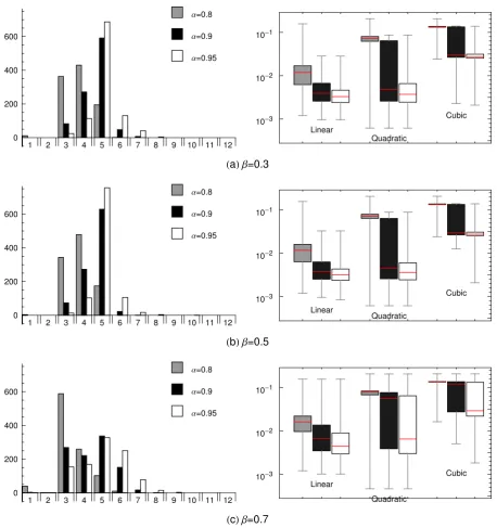
quadratic and cubic GeDS fits are presented in Figure 5, for choices of values of the parameter

α_{exit = 0}.8,0.9,0.95, and choices for parameter β= 0.3,0.5,0.7.

The frequency plots given in the left panels of Figure 5 show that for this test example a

choice of α_{exit = 0}.8 and 0.9 leads to a relative underfitting, more expressed for α_{exit = 0}.8,

whereas setting α_{exit = 0}.95 provides the best distribution of the number of knots, l, chosen

for the linear fit at the end of Stage A, and results in the lowest MSE values, in particular when

β = 0.5 or β = 0.3 (see the right panels of Figure 5). Let us compare these observations with

those related to the test example from section 4.1 in the paper. The noise level there is lower

(SNR=7) and good results are obtained withα_{exit = 0}.9 andβ = 0.5 orβ = 0.7. The latter is

intuitive, recalling that a higher value ofβputs more weight on the within-cluster mean relative

the right panels of Figure 5 illustrate that, for the particular level of smoothness of the test

function and the chosen SNR=5, the results forα_{exit = 0}.95 are substantially better than those

forα_{exit = 0}.8 and somewhat better than α_{exit = 0}.9, with the linear and the quadratic GeDS

fits being quite close.

1 2 3 4 5 6 7 8 9 10 11 12

Α=0.8

Α=0.9

Α=0.95

0 200 400 600

Linear

Quadratic

Cubic 10-1

10-2

10-3

HaLΒ=0.3

1 2 3 4 5 6 7 8 9 10 11 12

Α=0.8

Α=0.9

Α=0.95

0 200 400 600

Linear

Quadratic

Cubic 10-1

10-2

10-3

HbLΒ=0.5

1 2 3 4 5 6 7 8 9 10 11 12

Α=0.8

Α=0.9

Α=0.95

0 200 400 600

Linear

Quadratic

Cubic 10-1

10-2

10-3

HcLΒ=0.7

1 2 3 4 5 6 7 8 9 10 11 12 GCV,d(k)=k+1

GeDS,Α=0.95 ,Β=0.5

SURE,D=1.2

0 200 400 600

Linear

Quadratic

Cubic 10-1

10-2

10-3

HaLN=256 ,SNR=5

1 2 3 4 5 6 7 8 9 10 11 12 N=512 ,SNR=5 N=256 ,SNR=5 N=512 ,SNR=3

0 200 400 600

Linear

Quadratic

Cubic 10-1

10-2

10-3

HbLΑ=0.95 ,Β=0.5

1 2 3 4 5 6 7 8 9 10 11 12 N=512 ,SNR=5 N=256 ,SNR=5 N=512 ,SNR=3

0 200 400 600

Linear

Quadratic

Cubic 10-1

10-2

10-3

HcLΑ=0.95 ,Β=0.3

Figure 6: (Example 1) Frequency plots of the number of knots l (left panels) and box plots of the MSE values (right panels) of the 1000 GeD spline fits for: (a) - three different choices of model selection criterion; (b) and (c) - three different choices (combinations) of number of data,

In the top panel of Figure 6, the number of knots and the MSE values for the 1000 GeD

spline fits obtained with β = 0.5 and α_{exit = 0}.95, and illustrated in white in Figure 5 (b),

are compared with the results obtained applying the GeDS methodology to the same 1000 data

sets but with GCV and SURE as alternative model selection criteria. As noted in section 3 of

the paper, we have assumed that the minimum in SURE or GCV is attained when they do not

decrease in two consecutive iterations in stage A. As can be seen, the GCV, with a choice of

d(k) =k+ 1, leads to underfitting, and so does the SURE, with a choice ofD= 1.2, which also

results in a more dispersed distribution of the number of knots. Here, we used(k) =k+ 1 and

D = 1.2, since choices with higher penalization, e.g. D = 3 and d(k) = 3k+ 1, tend to more

often yield models underfitting the underlying function f, as noted by Zhou and Shen (2001).

Based on Example 1, the performance of GeDS is also tested when the number of simulated

data points increases and when the SNR worsens. The latter is achieved with ϵ∼N(0,0.42_).

Thus, in the middle and bottom panels of Figure 6, the results from Figure 5 (b) and (a),

obtained with α_{exit = 0}.95 (illustrated in white), are compared with the results from GeDS

method applied to twice as many data points (N = 512) with the same level of noise (SNR=5),

or a higher noise level, SNR=3. As expected, the MSE values improve for both β = 0.5 and

β = 0.3 when more data are used, see the gray boxes in Figure 6 (b) and (c) respectively, and

the results worsen when the noise level increases, see the white boxes in Figure 6 (b) and (c)

respectively.

Example 2. The function f2 (see Table 1) appears as a test example in Fan and Gijbels

(1995), Luo and Wahba (1997), Denison et al. (1998) and Zhou and Shen (2001). Using the

GeDS method we have produced linear, quadratic and cubic fits which are illustrated in Figure

7 and whose details are given in Table 5. It takes 1.68 seconds to compute fits No 1-3 and 1.97

seconds to compute fits No 4 and 5 of Table 5.

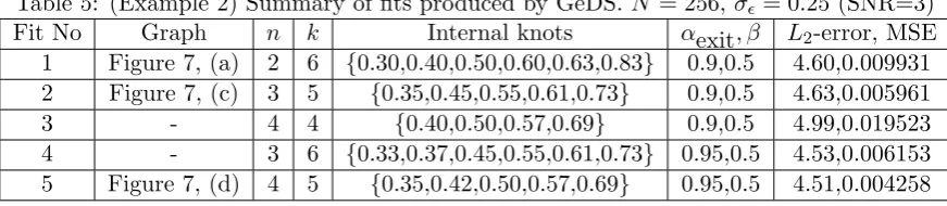
Table 5: (Example 2) Summary of fits produced by GeDS.N = 256,σϵ= 0.25 (SNR=3)

Fit No Graph n k Internal knots α_exit, β L2-error, MSE

1 Figure 7, (a) 2 6 {0.30,0.40,0.50,0.60,0.63,0.83} 0.9,0.5 4.60,0.009931 2 Figure 7, (c) 3 5 {0.35,0.45,0.55,0.61,0.73} 0.9,0.5 4.63,0.005961

3 - 4 4 {0.40,0.50,0.57,0.69} 0.9,0.5 4.99,0.019523

4 - 3 6 {0.33,0.37,0.45,0.55,0.61,0.73} 0.95,0.5 4.53,0.006153 5 Figure 7, (d) 4 5 {0.35,0.42,0.50,0.57,0.69} 0.95,0.5 4.51,0.004258

0.0 0.2 0.4 0.6 0.8 1.0

-1 0 1 2

HaL

Ÿ

Ÿ

Ÿ Ÿ

Ÿ Ÿ

Ÿ Ÿ Ÿ Ÿ

Αexit=0.9 Αexit=0.95

0 1 2 3 4 5 6 7 8 9

0.0 0.2 0.4 0.6 0.8 1.0

Number of knots

HbL

RSS



N

Α

0.0 0.2 0.4 0.6 0.8 1.0

-1 0 1 2

HcL

0.0 0.2 0.4 0.6 0.8 1.0

-1 0 1 2

HdL

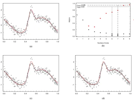
in Table 3. Sincef2 is also relatively smooth we have usedα_{exit = 0}.95 andβ= 0.5 in order to

obtain the cubic fit in Figure 7 (d), which has very good visual quality and low MSE value. The

GeD spline fits No 1-3 of Table 5, with number of regression functions k+n= 8, are obtained

with the default valuesα_{exit = 0}.9 andβ= 0.5. The cubic fit, No 3, with four knots, underfits

the data while, as seen from Figure 7 (a) and (c), the linear and quadratic fits are sufficiently

accurate, see also the results presented in Figure 8. Adding one more knot by running GeDS

with the higher value of α_{exit = 0}.95 improves the cubic fit as illustrated by Figure 7 (d). The

behavior of the proposed model selection criterion of Stage A (see eq. (10) in the paper), is

illustrated in Figure 7 (b). It can be seen that with α_{exit = 0}.9 the procedure exits with 6

internal knots for the linear fit and the RSS is 21.17. This means that the RSS of the linear fit

with 8 knots is at least 90% of the value 21.17, i.e., the residual sum of squares has stabilized

for three consecutive steps at which models with 6, 7 and 8 knots have been computed. If

α_{exit = 0}.95 the procedure exits one step later, with 7 internal knots for the linear fit and

RSS=20.38 since the improvement in RSS for the next two consecutive steps is less than 5% of

20.38. So, we see that the GeDS deviance-based model selector, tends to select models with an

appropriate number of knots. This is confirmed by the comparison of the GeDS model selection

with the alternative GCV and SURE criteria, given in Figure 9 (a).

Based on the L2-errors, given in Table 5, we have chosen the cubic GeD spline fit No 5 in

Table 5 to compare with the optimal cubic spline fits PNOM and NOM with the same number

of knots. The results are summarized in Table 6. As in Example 1, the GeD fit is better in

terms of MSE and visual quality. The location of the knots is similar for GeDS and PNOM (fit

No 2), both avoiding replicate knots. However, the optimal fit NOM (fit No 3) has 3 replicate

knots at 0.5 and hence, produces an edge and visually deviates more strongly from the shape

of the underlying function. The computation time needed for GeDS is less than two seconds

and for PNOM and NOM it is, respectively, 1.1 hours and 1.9 hours, using the Mathematica

functionNMinimize.

Table 6: (Example 2) The fits produced by GeDS, PNOM and NOM.

Fit No Method n k Internal knots L2-error, MSE

The robustness of the GeDS methodology with respect to the values of the parameters,

α_exit, β, is again investigated on the basis of 1000 simulated data sets and results are given in

Figure 8. Frequency plots of the number of internal knots of the 1000 linear GeD spline fits and

box plots of the MSE values of the linear, quadratic and cubic GeDS fits are presented in Figure

8, for choices of values α_{exit = 0}.8,0.9,0.95, andβ = 0.3,0.5,0.7. The frequency plots and the

MSE values, given in the left and right panels of Figure 8 show that, for the particular level

of smoothness of the test function and the chosen SNR=3, a choice of α_{exit = 0}.95 provides

the best distribution of the number of knots, l, chosen for the linear fit at the end of Stage A,

in particular when β = 0.5 or β = 0.3, and results in somewhat lower MSE values than those

for α_{exit = 0}.8 andα_{exit = 0}.9, with the latter fits being quite close (see the gray and black

box plots presented in the right panels of Figure 8). Note that these conclusions are similar to

those related to Example 1 where the noise level is slightly lower (SNR=5). The median MSE

value for the 1000 linear and quadratic fits with α_{exit = 0}.95, β = 0.3 (see top right panel in

Figure 8) are equal to 0.007 and 0.009 respectively, and are comparable with those produced

by other authors. For example, Luo and Wahba (1997) report MSE=0.007 and number of basis

functions equal to 13 for their HAS models. For all 1000 linear fits the number of internal knots

used by GeDS is between 2 and 12.

Similarly to Example 1, the number of knots and the MSE values for the 1000 GeD spline fits

obtained withβ = 0.3 andα_{exit = 0}.95, and illustrated in white in Figure 8 (a), are compared

with the results obtained applying the GeDS methodology to the same 1000 data sets but with

GCV and SURE as alternative model selection criteria; see the top panel of Figure 9. As can

be seen, the GCV, with a choice of d(k) = k+ 1, and the SURE, with a choice of D = 1.2,

produce very similar MSE values for each of the linear, quadratic and cubic GeDS fits, again

with the SURE leading to a more dispersed distribution of the number of knots.

Based on Example 2, the performance of GeDS is again tested when the number of simulated

data points increases and when SNR worsens. The latter is achieved withϵ∼N(0,0.42). Thus,

in the middle and bottom panels of Figure 9, the results from Figure 8 (a) and (b), obtained

withα_{exit = 0}.95 (illustrated in white), are compared with the results from the GeDS method

applied to twice as many data points (N = 512) with the same level of noise (SNR=3), or a

higher noise level, SNR=2. As expected, the MSE values somewhat improve for both β = 0.3

1 2 3 4 5 6 7 8 9 10 11 12 Α=0.8 Α=0.9 Α=0.95 0 100 200 300 400 500 600 700 Linear Quadratic Cubic 10-1 10-2 10-3

HaLΒ=0.3

1 2 3 4 5 6 7 8 9 10 11 12

Α=0.8 Α=0.9 Α=0.95 0 100 200 300 400 500 600 700 Linear Quadratic Cubic 10-1 10-2 10-3

HbLΒ=0.5

1 2 3 4 5 6 7 8 9 10 11 12

Α=0.8 Α=0.9 Α=0.95 0 100 200 300 400 500 600 700 Linear _Quadratic Cubic 10-1

10-2

10-3

HcLΒ=0.7

1 2 3 4 5 6 7 8 9 10 11 12 GCV,d(k)=k+1

GeDS,Α=0.95 ,Β=0.3

SURE,D=1.2

0 100 200 300 400

Linear

Quadratic _Cubic 10-1

10-2

10-3

HaLN=256 ,SNR=3

1 2 3 4 5 6 7 8 9 10 11 12 N=512 ,SNR=3 N=256 ,SNR=3 N=512 ,SNR=2

0 100 200 300 400

Linear

Quadratic

Cubic 10-1

10-2

10-3

HbLΑ=0.95 ,Β=0.3

1 2 3 4 5 6 7 8 9 10 11 12 N=512 ,SNR=3 N=256 ,SNR=3 N=512 ,SNR=2

0 100 200 300 400

Linear

Quadratic

Cubic 10-1

10-2

10-3

HcLΑ=0.95 ,Β=0.5

Figure 9: (Example 2) Frequency plots of the number of knots l (left panels) and box plots of the MSE values (right panels) of the 1000 GeD spline fits for: (a) - three different choices of model selection criterion; (b) and (c) - three different choices (combinations) of number of data,

and the results worsen significantly when the noise level increases; see the white boxes in Figure

9 (b) and (c) respectively.

Example 3. The HeaviSine function is one of the four functions introduced by Donoho and Johnstone

(1994) and widely used as test examples by other authors, see for example Fan and Gijbels

(1995), Luo and Wahba (1997), Denison et al. (1998), Zhou and Shen (2001), Lee (2000, 2002a,b),

Pittman (2002). It is a smooth function with two discontinuities atx= 0.3 and x= 0.72.

HeaviSine,Β=0.5

10 15 20 25 30

Α=0.95

0 5 10 15 20

10 15 20 25 30

Α=0.99

0 5 10 15 20

10 15 20 25 30

Α=0.995

0 5 10 15 20

Linear

Quadratic Cubic 0.0

0.1 0.2 0.3 0.4 0.5

Figure 10: (Example 3) Frequency plots of the number of knots l and box plots of the MSE values of the 100 GeD spline fits obtained with three different choices of values of the parameter

α_{exit, and} β = 0.5.

As with the previous examples, the sensitivity of the GeD spline estimator with respect to the

value of the model selection parameter,α_{exit, is investigated on the basis of 100 simulated data}

sets and results are given in Figure 10. Frequency plots of the number of internal knots of the 100

linear GeD spline fits and box plots of the MSE values of the linear, quadratic and cubic GeDS

fits are presented in Figure 10, for choices of values of the parameter α_{exit = 0}.95,0.99,0.995.

The frequency plots and the MSE values, given in Figure 10, show that, for the particular level

of smoothness of the test function and the chosen SNR=7, a choice of α_{exit = 0}.99 provides

and results in much lower MSE values than those forα_{exit = 0}.95 and somewhat comparable

values to those for α_{exit = 0}.995 (see the black and white box plots presented in the bottom

right panel of Figure 10). As seen in this and the following examples of spatially inhomogeneous

curves, a value ofα_exit≤0.95 would lead to underfitting, and hence, to a spline approximation

of the data which does not adequately represent their ‘shape’.

Table 7: (Example 3) Summary of fits produced by GeDS.

Fit Graph n k Internal knots α_exit, β L2-error

No MSE

1 - 2 18 {0.10,0.13,0.18,0.29,0.30,0.30,0.32,0.38,0.44, 0.99,0.5 46.56 0.57,0.63,0.71,0.71,0.72,0.74,0.83,0.84,0.99} 0.2203 2 Figure 11 3 17 {0.11,0.16,0.23,0.29,0.30,0.31,0.35,0.41,0.50, 0.99,0.5 43.42

0.60,0.67,0.71,0.72,0.73,0.79,0.84,0.92} 0.0482 3 - 4 16 {0.14,0.20,0.26,0.30,0.31,0.33,0.38,0.46,0.55, 0.99,0.5 44.82

0.64,0.69,0.72,0.73,0.77,0.81,0.89} 0.0942

0.0 0.2 0.4 0.6 0.8 1.0

-15 -10 -5 0 5 10

Figure 11: (Example 3) Graph of the quadratic GeD spline fit, specified in Table 7. The dotted function is the true function.

The median MSE value for the 100 quadratic fit (withα_{exit = 0}.99,β = 0.5) is equal to 0.05,

and is comparable with 0.04 given by Luo and Wahba (1997) for their cubic spline model with

50 basis functions, and with the minimum median MSE of 0.08 reported by Lee (2002b) (note

the scaling adjustment of the reportedM SE= 8.46 in Lee (2002b) as 0.08 = (8.46/512)∗2.22).

MSE respectively) which could partially be due to difference in the number of simulations, 100

instead of 50 as in Lee (2002a). Unfortunately, Lee (2002a,b) does not give the number of knots

used. Our GeDS algorithm uses between 13 and 26 internal knots to fit the 100 simulated data

sets in the linear case. A quadratic GeDS fit with a (median) number of regression functions

k+n= 20 and a (median) MSE value of 0.0482 (see fit No 2 in Table 7), is illustrated in Figure

11. It takes 46 seconds to obtain simultaneously the linear, quadratic and cubic GeD spline

fits, given in Table 7. Based on the MSE values illustrated in the bottom right panel of Figure

10 and the L2-errors for the linear, quadratic and cubic fits given in Table 7, the best GeDS

approximation for this particular function is of degree 2. It should be noted that a quadratic

spline fit to the data with 17 uniform knots results inL2-error of 47.33 and MSE value of 0.2281.

Example 4. This function is known as the Doppler function. It is highly oscillating,

espe-cially near the origin, where most of the procedures fail to recover it. Here again, the sensitivity

of the GeD spline estimator with respect to the value of the model selection parameter,α_exit,

is investigated on the basis of 100 simulated data sets. Frequency plots of the number of

in-ternal knots of the 100 linear GeD spline fits and box plots of the MSE values of the linear,

quadratic and cubic GeDS fits are presented in Figure 12, for choices of values of the parameter

α_{exit = 0}.99,0.995,0.999 and β = 0.5. The frequency plots and the MSE values show that

for the particular level of wiggliness of the test function and the chosen SNR=7, a choice of

α_{exit = 0}.999 provides the lowest MSE values (see the white box plots presented in the bottom

right panel of Figure 12), although the corresponding distribution of the number of knots, l,

chosen for the linear fit at the end of Stage A, is more dispersed than the one for α_{exit = 0}.99

or α_{exit = 0}.995. Based on the MSE values illustrated in the bottom right panel of Figure

12 and the L2-errors for the linear, quadratic and cubic fits given in Table 8, the best GeDS

approximation for this particular function is of degree 2.

The median MSE value for the 100 quadratic fits (with α_{exit = 0}.999, β = 0.5) is equal to

0.085, and the median number of knots is 62, although it is quite spread, varying between 33

and 91. These figures are somewhat smaller compared to the HAS cubic fit with MSE=0.10

and 120 basis functions, produced by Luo and Wahba (1997), and compared to the minimum

median MSE of 0.17 reported by Lee (2002b) for the MDL method (note the scaling adjustment

of the reported M SE= 0.18 in Lee (2002b) as 0.17 = (0.18/512)∗222).

Doppler,Β=0.5

25 30 35 40 45 50 55 60 65 70 75 80 85 90 95

Α=0.99

0 2 4 6 8 10

25 30 35 40 45 50 55 60 65 70 75 80 85 90 95

Α=0.995

0 2 4 6 8 10

25 30 35 40 45 50 55 60 65 70 75 80 85 90 95

Α=0.999

0 2 4 6 8 10

Linear

Quadratic Cubic

0.0 0.1 0.2 0.3 0.4 0.5

Figure 12: (Example 4) Frequency plots of the number of knots l and box plots of the MSE values of the 100 GeD spline fits obtained with three different choices of values of the parameter

α_{exit, and} β = 0.5.

Table 8: (Example 4) Summary of fits produced by GeDS. Fit No Graph n k α_exit, β L2-error, MSE

1 - 2 47 0.99,0.5 48.24,0.199802

2 - 3 46 0.99,0.5 46.77,0.125328

3 - 4 45 0.99,0.5 49.04,0.233945

4 - 2 74 0.999,0.5 45.21,0.114633

5 Figure 13 3 73 0.999,0.5 44.92,0.060037

0.0 0.2 0.4 0.6 0.8 1.0 -10

-5 0 5 10

Figure 13: (Example 4) Graph of the quadratic GeD spline fit, specified in Table 8. The dotted function is the true function.

data set andα_{exit = 0}.99 orα_{exit = 0}.999, are presented in Table 8. Fits No 1-3 are calculated

simultaneously in 179 seconds with α_{exit = 0}.99 and fits No 4-6 are calculated simultaneously

in 381 seconds with α_{exit = 0}.999. The quadratic GeD spline fit No 5, with 73 knots and

MSE=0.06, is plotted in Figure 13 and is seen to fit very well the Doppler function near the

origin, avoiding under/oversmoothing. Note that a quadratic spline fit to the data with 46 (73)

uniform knots leads to L2-error of 90.38 (76.09) and MSE value of 3.11 (1.96).

Example 5. The Bumps function is very wiggly and also difficult to fit. The robustness

of the GeD spline estimator with respect to the value of the model selection parameter,α_exit,

is investigated on the basis of 100 simulated data sets. Frequency plots of the number of

internal knots of the 100 linear GeD spline fits and box plots of the MSE values of the linear,

quadratic and cubic GeDS fits are presented in Figure 14, for choices of values of the parameter

α_{exit = 0}.99,0.995,0.999 and β = 0.5. The frequency plots and the MSE values show that

for the particular level of wiggliness of the test function and the chosen SNR=7, a choice of

α_{exit = 0}.999 provides the lowest MSE values (see the white box plots presented in the bottom

right panel of Figure 14), and also gives a good distribution of the number of knots, l, chosen

for the linear fit at the end of Stage A. Note that the choice of α_{exit = 0}.99 and α_{exit = 0}.995

leads to several spline fits with very small number of knots (relative to the wiggliness of the

Bumps,Β=0.5

5 15 25 35 45 55 65 75 85 95 105 115

Α=0.99

0 2 4 6 8 10

5 15 25 35 45 55 65 75 85 95 105 115

Α=0.995

0 2 4 6 8 10

5 15 25 35 45 55 65 75 85 95 105 115

Α=0.999

0 2 4 6 8 10

Linear Quadratic

Cubic 0.0

0.5 1.0 1.5 2.0 2.5

Figure 14: (Example 5) Frequency plots of the number of knots l and box plots of the MSE values of the 100 GeD spline fits obtained with three different choices of values of the parameter

α_{exit, and} β = 0.5.

In the case of Bumps, the GeD spline approximation with the lowest median MSE values

is the linear one. This is confirmed by the MSE values illustrated in the bottom right panel of

Figure 14 and the L2-errors of the linear, quadratic and cubic fits, specified in Table 9. The

linear GeD spline fit No 4 is illustrated in Figure 15. A linear fit for Bumps is given also by

Lee (2000) whose MDL procedure automatically chooses the order of the fit within the range

1 to 4. Based on the 100 simulated data sets (with α_{exit = 0}.999, β = 0.5), the median MSE

value for the linear fit is 0.23 (for the quadratic fit it is 0.49) and the median number of knots is

91, ranging between 70 and 115. For comparison, the median MSE value reported by Pittman

(2002) for the cubic AGS fit is 0.4001, for a certain median number of knots, which is not

reported. Also, the minimum median MSE reported by Lee (2002b) is 0.67 (note the scaling

adjustment of the reportedM SE= 3.41 in Lee (2002b) as 0.08 = (3.41/512)∗102). Fits No 1-3

are obtained simultaneously in 410 seconds, whereas fits No 4-6 are computed in 622 seconds.

Furthermore, a linear spline fit to the data with 83 (103) uniform knots results in L2-error of

Table 9: (Example 5) Summary of fits produced by GeDS. Fit No Graph n k α_exit, β L2-error, MSE

1 - 2 83 0.99,0.5 48.59,0.283631

2 - 3 82 0.99,0.5 56.03,0.631448

3 - 4 81 0.99,0.5 66.44,1.198390

4 Figure 15 2 103 0.999,0.5 44.51,0.140580

5 - 3 102 0.999,0.5 47.96,0.264664

6 - 4 101 0.999,0.5 52.29,0.445403

0.0 0.2 0.4 0.6 0.8 1.0

0 10 20 30 40 50

Figure 15: (Example 5) Graph of the linear GeD spline fit No 4, specified in Table 9. The dotted function is the true function.

Example 6. The last test example is based on the Blocks function. Again, on the basis of

100 simulated data sets (SNR=7), the robustness of the GeD spline estimator is investigated

with respect to the choice of value for the model selection parameter,α_exit.

Frequency plots of the number of internal knots of the 100 linear GeD spline fits and box

plots of the MSE values of the linear, quadratic and cubic GeDS fits are presented in Figure 16,

for choices of the parameter α_{exit = 0}.99,0.995,0.999 and β = 0.5. A choice ofα_{exit = 0}.999

provides the lowest MSE values (see the white box plots presented in the bottom right panel of

Figure 16), but with a relatively dispersed distribution of the number of knots,l, chosen for the

linear fit at the end of Stage A. Based on the MSE values illustrated in the bottom right panel

of Figure 16 and theL2-errors for the linear and quadratic fits given in Table 10, the best GeDS

withα_{exit = 0}.999, is 0.14 with 80 median number of knots. For comparison, the median MSE

value given by Zhou and Shen (2001) is 0.08, who do not report the number of knots of their

SARS fit, and the minimum median MSE reported by Lee (2002b) is also 0.08 (note the scaling

adjustment of the reportedM SE = 3.41 in Lee (2002b) as 0.08 = (3.41/512)∗3.52)

The details of two pairs of linear and quadratic fits for α_{exit = 0}.99 and α_{exit = 0}.999

respectively, are presented in Table 10. The GeD linear spline fit No 3 is illustrated in Figure

17. Fits No 1-2 are obtained in 198 seconds and No 3-4 in 434 seconds. Note that a linear spline

fit to the data with 53 (85) uniform knots results in L2-error of 101.79 (81.13) and MSE value

of 3.99 (2.31).

Blocks,Β=0.5

30 40 50 60 70 80 90 100

Α=0.99

0 2 4 6 8 10 12

30 40 50 60 70 80 90 100

Α=0.995

0 2 4 6 8 10 12

30 40 50 60 70 80 90 100

Α=0.999

0 2 4 6 8 10 12

Linear Quadratic

Cubic 0.0

0.5 1.0 1.5 2.0 2.5

Figure 16: (Example 6) Frequency plots of the number of knots l and box plots of the MSE values of the 100 GeD spline fits obtained with three different choices of values of the parameter

α_{exit, and} β = 0.5.

Table 10: (Example 6) Summary of fits produced by GeDS. Fit No Graph n k α_exit, β L2-error, MSE

1 - 2 53 0.99,0.5 55.63,0.642906

2 - 3 52 0.99,0.5 59.80,0.860989

3 Figure 17 2 85 0.999,0.5 42.43,0.082962

0.0 0.2 0.4 0.6 0.8 1.0 -10

-5 0 5 10 15 20

References

De Boor, C. (2001).A practical Guide to Splines, Revised Edition, New York: Springer.

Denison, D., Mallick, B., and Smith, A. (1998). Automatic Bayesian curve fitting,J. R. Statist. Soc., B,60, 333–350.

Donoho, D. and Johnstone, I. (1994). Ideal spatial adaptation by wavelet shrinkage.Biometrika,

81, 425–455.

Fan, J. and Gijbels, I. (1995). Data-driven bandwidth selection in local polynomial fitting: Variable bandwidth and spatial adaptation. J. R. Statist. Soc., B,57, 371–394.

Farin, G. (2002). Curves and Surfaces for CAGD, Fifth Edition, San Francisco: Morgan Kauf-mann.

Jupp, D. (1978). Approximation to data by splines with free knots. SIAM J. Num. Analysis,

15, 328–343.

Lee, T. C. M. (2000). Regression spline smoothing using the minimum description length prin-ciple. Stat. & Prob. Letters,48, 71–82.

Lee, T. C. M. (2002a). Automatic smoothing for discontinuous regression functions.Stat. Sinica,

12, 823–842.

Lee, T. C. M. (2002b). Automatic smoothing for discontinuous regression functions: Supporting document. Available at: _{http://anson.ucdavis.edu/~tcmlee/PSfiles/support.ps.gz}.

Lee, T. C. M. (2002c). On algorithms for ordinary least squares regression spline fitting: A comparative study.J. of Stat. Comp. and Simulation,72, 647–663.

Lindstrom, M. J. (1999). Penalized estimation of free-knot splines.J. Comput. and Graph. Stat.,

8, 2, 333–352.

Luo, Z., and Wahba, G. (1997). Hybrid adaptive splines.J. Am. Statist. Ass.,92, 107–115.

Micchelli, C. A., Rivlin, T.J. and Winograd, S. (1976). The optimal recovery of smooth func-tions. Numer. Math.,26, 191–200.

Pittman, J. (2002). Adaptive Splines and Genetic Algorithms. J. Comput. and Graph. Stat.,

11, 3, 1–24.

Ruppert, D., Sheather, S. J. and Wand, M. P. (1995). An effective bandwidth selector for local least squares regression. J. Amer. Statist. Assoc.90, 1257–1270.

Smith, M. and Kohn, R. (1996). Nonparametric regression using Bayesian variable selection.J. Econometrics,75, 317–344.