MOOC
massive open online calculus
ULUS
C A L C U L U S
Copyright c 2014 Jim Fowler and Bart Snapp
This work is licensed under the Creative Commons Attribution-NonCommercial-ShareAlike License. To view a copy of this license, visithttp://creativecommons.org/licenses/by-nc-sa/3.0/or send a letter to Creative Commons, 543 Howard Street, 5th Floor, San Francisco, California, 94105, USA. If you distribute this work or a derivative, include the history of the document.
The source code is available at: https://github.com/ASCTech/mooculus/tree/master/public/textbook
This text is based on David Guichard’s open-source calculus text which in turn is a modification and expansion of notes written by Neal Koblitz at the University of Washington. David Guichard’s text is available athttp://www.whitman.edu/mathematics/ calculus/under a Creative Commons license.
The book includes some exercises and examples fromElementary Calculus: An Approach Using Infinitesimals, by H. Jerome Keisler, available athttp://www.math.wisc.edu/~keisler/calc.htmlunder a Creative Commons license.
This book is typeset in the Kerkis font, Kerkis c Department of Mathematics, University of the Aegean.
0
Functions
8
1
Limits
19
2
Infinity and Continuity
36
3
Basics of Derivatives
47
4
Curve Sketching
64
5
The Product Rule and Quotient Rule
82
7
The Derivatives of Trigonometric Functions and their Inverses
107
8
Applications of Differentiation
121
9
Optimization
146
10
Linear Approximation
161
11
Antiderivatives
178
12
Integrals
197
13
The Fundamental Theorem of Calculus
208
14
Techniques of Integration
219
15
Applications of Integration
235
Answers to Exercises
245
1.3.1 Limit Laws . . . 30
1.3.5 Squeeze Theorem . . . 32
2.3.3 Intermediate Value Theorem . . . 44
3.1.3 Differentiability Implies Continuity . . . 50
3.2.1 The Constant Rule . . . 55
3.2.2 The Power Rule . . . 56
3.2.6 The Sum Rule . . . 58
3.2.9 The Derivative ofex . . . . 60
4.1.1 Fermat’s Theorem . . . 65
4.2.1 First Derivative Test. . . 68
4.3.1 Test for Concavity . . . 72
4.4.1 Second Derivative Test . . . 75
5.1.1 The Product Rule . . . 83
5.2.1 The Quotient Rule. . . 86
6.1.1 Chain Rule. . . 90
6.2.2 The Derivative of the Natural Logrithm . . . 99
6.2.3 Inverse Function Theorem . . . 100
7.1.5 The Derivatives of Trigonometric Functions . . . 111
7.2.4 The Derivatives of Inverse Trigonometric Functions . . . 119
8.1.1 L’Hôpital’s Rule . . . 121
9.1.1 Extreme Value Theorem . . . 147
10.3.1 Rolle’s Theorem . . . 173
11.1.1 Basic Antiderivatives . . . 179
11.1.2 The Sum Rule for Antiderivatives . . . 179
12.1.3 Properties of Definite Integrals . . . 198
13.1.1 Fundamental Theorem of Calculus—Version I . . . 208
13.1.2 Fundamental Theorem of Calculus—Version II . . . 210
14.1.1 Integral Substitution Formula . . . 219
Reading mathematics isnotthe same as reading a novel. To read mathematics you need:
(a) A pen.
(b) Plenty of blank paper.
(c) A willingness to write things down.
0.1
For Each Input, Exactly One Output
Life is complex. Part of this complexity stems from the fact that there are many relations between seemingly independent events. Armed with mathematics we seek
to understand the world, and hence we need tools for talking about these relations. Something as simple as a dictionary could be thought of as a relation, as it connectswordstodefinitions. However, a dictionary is not a function, as there are words with multiple definitions. On the other hand, if each word only had a single definition, then it would be a function.
A function is a relation between sets of objects that can be thought of as a “mathematical machine.” This means for each input, there is exactly one output.
Let’s say this explicitly.
Definition Afunctionis a relation between sets, where for each input, there is exactly one output.
Moreover, whenever we talk about functions, we should try to explicitly state what type of things the inputs are and what type of things the outputs are. In calculus, functions often define a relation from (a subset of) the real numbers to (a subset of) the real numbers.
While the name of the function is technically “f,” we will abuse notation and call the function “f(x)” to remind the reader that it is a function.
Example 0.1.1 Consider the functionf that maps from the real numbers to the real numbers by taking a number and mapping it to its cube:
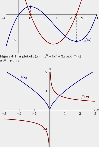
and so on. This function can be described by the formulaf(x)=x3or by the plot shown in Figure1.
Warning A function is a relation (such that for each input, there is exactly one output) between sets and should not be confused with either its formula or its plot.
• A formula merely describes the mapping using algebra. • A plot merely describes the mapping using pictures.
−2 −1 1 2
−5 5
x y
Figure 1: A plot off(x)=x3. Here we can see that for each input (a value on thex-axis), there is exactly one output (a value on they-axis).
Example 0.1.2 Consider thegreatest integer function, denoted by
f(x)=⌊x⌋.
This is the function that maps any real numberxto the greatest integer less than or equal tox. See Figure2for a plot of this function. Some might be confused because here we have multiple inputs that give the same output. However, this is not a problem. To be a function, we merely need to check that for each input, there is exactly one output, and this is satisfied.
−2 −1 1 2 3 4
−2
−1 1 2 3
x y
Figure 2: A plot off(x)=⌊x⌋. Here we can see that for each input (a value on thex-axis), there is exactly one output (a value on they-axis).
Just to remind you, a function maps from one set to another. We call the set a function is mapping from thedomainorsourceand we call the set a function is mapping to therangeortarget. In our previous examples the domain and range have both been the real numbers, denoted byR. In our next examples we show that this is not always the case.
Example 0.1.3 Consider the function that maps non-negative real numbers to their positive square root. This function is denoted by
f(x)= √x.
Note, since this is a function, and its range consists of the non-negative real numbers, we have that
√
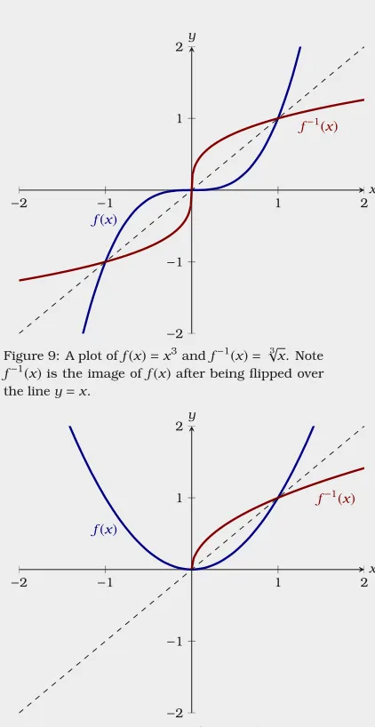
See Figure3for a plot off(x)= √x.
Finally, we will consider a function whose domain is all real numbers except for a single point.
Example 0.1.4 Consider the function defined by
f(x)=x
2
−3x+2
x−2
This function may seem innocent enough; however, it is undefined atx =2.
See Figure4for a plot of this function. −8 −6 −4 −2 2 4 6 8
−4
−2 2 4
x y
Figure 3: A plot off(x)=√x. Here we can see that for each input (a non-negative value on thex-axis), there is exactly one output (a positive value on the
y-axis).
−2 −1 1 2 3 4
−3
−2
−1 1 2 3
x y
Figure 4: A plot off(x) = x
2
−3x+2
Exercises for Section 0.1
−1 1 2 3 4
−1 1 2 3 4
[image:11.792.467.671.75.445.2]x y
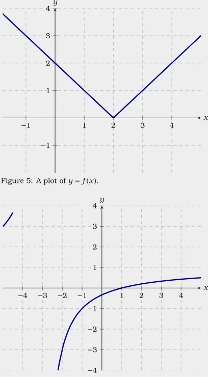
Figure 5: A plot ofy=f(x).
(1) In Figure5we see a plot ofy=f(x). What isf(4)?
➠
−4 −3 −2 −1 1 2 3 4
−4
−3
−2
−1 1 2 3 4
[image:11.792.76.537.85.538.2]x y
Figure 6: A plot ofy=f(x).
(2) In Figure6we see a plot ofy=f(x). What isf(−2)?
➠
(3) Consider the following points:
(5,8), (3,6), (−6,−9), (−1,−4), (−10,7)
Could these points all be on the graph of a functiony=f(x)?
➠
(4) Consider the following points:
(7,−4), (0,3), (−2,−2), (−1,−8), (10,4)
Could these points all be on the graph of a functiony=f(x)?
➠
(5) Consider the following points that lie on the graph ofy=f(x):
(−5,8), (5,−1), (−4,0), (2,−9), (4,10)
Iff(x)=−9 find the value ofx.
➠
(6) A student thinks the set of points does not define a function:
(−7,−4), (10,−4), (0,−4), (3,−4)
They argue that the output−4 has four different inputs. Are they correct?
➠
(7) Consider the following points:
(−1,5), (−3,4), (x,3), (5,−3), (8,5)
Name a value ofxso that these points do not define a function.
➠
(8) Letf(x)=18x5−27x4−32x3+11x2−7x+4. Evaluatef(0).
➠
(9) Letf(x)=x5+2x4+3x3+4x2+5x+6. Evaluatef(1).
➠
(10) Letf(x)=x5+2x4+3x3+4x2+5x+6. Evaluatef(−1).
➠
(11) Letf(x)=√x2+x+1. Evaluatef(w).
➠
(12) Letf(x)=√x2+x+1. Evaluatef(x+h).
➠
(14) Letf(x)=x+1. What isf(f(f(f(1))))?
➠
(15) Letf(x)=x+1. What isf(f(f(f(x+h))))?
➠
(16) Iff(8)=8 andg(x)=3·f(x), what point must satisfyy=g(x)?
➠
(17) Iff(7)=6 andg(x)=f(8·x), what point must satisfyy=g(x)?
➠
0.2
Inverses of Functions
If a function maps every input to exactly one output, an inverse of that function maps every “output” to exactly one “input.” While this might sound somewhat esoteric, let’s see if we can ground this in some real-life contexts.
Example 0.2.1 Suppose that you are filling a swimming pool using a garden hose—though because it rained last night, the pool starts with some water in it. The volume of water in gallons afterthours of filling the pool is given by:
v(t)=700t+200
What does the inverse of this function tell you? What is the inverse of this function?
Here we abuse notation slightly, allowingvandtto simultaneously be names of variables and functions. This is standard practice in calculus classes.
Solution While v(t)tells you how many gallons of water are in the pool after
a period of time, the inverse of v(t)tells you how much time must be spent to obtain a given volume. To compute the inverse function, first set v=v(t)and write
v=700t+200. Now solve for t:
t=v/700−2/7
This is a function that maps volumes to times, andt(v)=v/700−2/7. Now let’s consider a different example.
Example 0.2.2 Suppose you are standing on a bridge that is 60 meters above sea-level. You toss a ball up into the air with an initial velocity of 30 meters per second. Iftis the time (in seconds) after we toss the ball, then the height at timetis approximatelyh(t)=−5t2+30t+60. What does the inverse of this function tell you? What is the inverse of this function?
Solution Whileh(t)tells you how the height the ball is above sea-level at an
of h(t). Consider Figure7, we can see that for some heights—namely 60 meters, there are two times.
While there is no inverse function for h(t), we can find one if we restrict the domain of h(t). Take it as given that the maximum of h(t)is at105meters and t=3seconds, later on in this course you’ll know how to find points like this with ease. In this case, we may find an inverse of h(t)on the interval[3,∞). Write
h=−5t2+30t+60 0=−5t2+30t+(60−h)
and solve for t using the quadratic formula
t= −30± p
302−4(−5)(60−h)
2(−5) = −30±
p
302+20(60−h)
−10 =3∓p32+.2(60−h)
=3∓p9+.2(60−h) =3∓√21−.2h
Now we must think about what it means to restrict the domain of h(t)to values of t in[3,∞). Since h(t)has its maximum value of105when t=3, the largest h could be is105. This means that21−.2h ≥0and so √21−.2h is a real number. We know something else too, t > 3. This means that the “∓” that we see above must be a “+.” So the inverse of h(t)on the interval[3,∞)is t(h)=3+√21−.2h. A similar argument will show that the inverse of h(t)on the interval(−∞,3]is t(h)=3−√21−.2h.
2 4 6
20 40 60 80 100 t h
Figure 7: A plot ofh(t)=−5t2+30t+60. Here we can see that for each input (a value on thet-axis), there is exactly one output (a value on theh-axis). However, for each value on thehaxis, sometimes there are two values on thet-axis. Hence there is no function that is the inverse ofh(t).
2 4 6
20 40 60 80 100 t h
Figure 8: A plot ofh(t)=−5t2+30t+60. While this plot passes the vertical line test, and hence representshas a function oft, it does not pass the horizontal line test, so the function is not one-to-one.
We see two different cases with our examples above. To clearly describe the difference we need a definition.
You may recall that a plot givesyas a function ofxif every vertical line crosses the plot at most once, this is commonly known as the vertical line test. A function is one-to-one if every horizontal line crosses the plot at most once, which is commonly known as the horizontal line test, see Figure8. We can only find an inverse to a function when it is one-to-one, otherwise we must restrict the domain as we did in Example0.2.2.
Let’s look at several examples.
Example 0.2.3 Consider the function
f(x)=x3.
Doesf(x)have an inverse? If so what is it? If not, attempt to restrict the domain off(x)and find an inverse on the restricted domain.
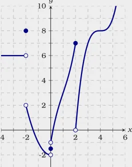
Solution In this case f(x)is one-to-one and f−1(x)=√3x. See Figure9.
−2 −1 1 2
−2
−1 1 2
f(x)
f−1(x)
[image:15.792.466.677.87.496.2]x y
Figure 9: A plot off(x)=x3andf−1(x)=√3x. Note
f−1(x)is the image off(x)after being flipped over
the liney=x. Example 0.2.4 Consider the function
f(x)=x2.
Doesf(x)have an inverse? If so what is it? If not, attempt to restrict the domain off(x)and find an inverse on the restricted domain.
Solution In this case f(x)is not one-to-one. However, it is one-to-one on the
interval[0,∞). Hence we can find an inverse of f(x)=x2on this interval, and it is our familiar function √x. See Figure10.
−2 −1 1 2
−2
−1 1 2
f(x)
f−1 (x)
x y
Figure 10: A plot off(x) =x2 andf−1(x) = √x. Whilef(x)=x2is not one-to-one onR, it is one-to-one on[0,∞).
0.2.1 A Word on Notation
Given a functionf(x), we have a way of writing an inverse off(x), assuming it exists
f−1(x)=the inverse off(x), if it exists. On the other hand,
f(x)−1= 1
Warning It is not usually the case that
f−1(x)=f(x)−1.
This confusing notation is often exacerbated by the fact that
sin2(x)=(sin(x))2 but sin−1(x),(sin(x))−1.
Exercises for Section 0.2
(1) The length in centimeters of Rapunzel’s hair aftertmonths is given by
ℓ(t)=8t 3 +8.
Give the inverse ofℓ(t). What does the inverse ofℓ(t)represent?
➠
(2) The value of someone’s savings account in dollars is given by
m(t)=900t+300
where t is time in months. Give the inverse ofm(t). What does the inverse ofm(t) represent?
➠
(3) At graduation the students all grabbed their caps and threw them into the air. The height of their caps can be described by
h(t)=−5t2+10t+2
whereh(t)is the height in meters andtis in seconds after letting go. Given that this h(t)attains a maximum at(1,7), give two different inverses on two different restricted domains. What do these inverses represent?
➠
(4) The numbernof bacteria in refrigerated food can be modeled by
n(t)=17t2−20t+700
wheretis the temperature of the food in degrees Celsius. Give two different inverses on two different restricted domains. What do these inverses represent?
➠
(5) The height in meters of a person off the ground as they ride a Ferris Wheel can be modeled by
h(t)=18·sin(π·t 7 )+20
wheretis time elapsed in seconds. Ifhis restricted to the domain[3.5,10.5], find and interpret the meaning ofh−1
(20).
➠
(6) The valuevof a car in dollars aftertyears of ownership can be modeled by
v(t)=10000·0.8t.
(7) The loudnessd(in decibels) is given by the equation
d(I)=10·log10 I I0
!
where I is the given intensity andI0 is the threshold sound (the quietest detectable intensity). Determined−1(85)in terms of the threshold sound.
➠
(8) What is the difference in meaning betweenf−1(x)andf(x)−1?
➠
(9) Sort the following expressions into two equivalent groups:
sin2x, sin(x)2, (sinx)2, sin(x2), sinx2, (sinx)(sinx)
➠
(10) Sort the following expressions into two equivalent groups:
arcsin(x), (sinx)−1,
sin−1(x), 1 sin(x)
➠
(11) Is √x2
1 Limits
1.1
The Basic Ideas of Limits
Consider the function:
f(x)= x
2
−3x+2
x−2
Whilef(x)is undefined atx=2, we can still plotf(x)at other values, see Figure1.1. Examining Table1.1, we see that asx approaches 2,f(x)approaches 1. We write this:
Asx→2,f(x)→1 or lim
x→2f(x)=1.
Intuitively, lim
x→af(x)=L when the value off(x)can be made arbitrarily close toL by making x sufficiently close, but not equal to, a. This leads us to the formal definition of alimit.
−2 −1 1 2 3 4
−3
−2
−1 1 2
x
Figure 1.1: A plot off(x)=x
2
−3x+2
x−2 .
x f(x)
1.7 0.7 1.9 0.9 1.99 0.99 1.999 0.999 2 undefined
x f(x)
2 undefined 2.001 1.001 2.01 1.01 2.1 1.1 2.3 1.3
Table 1.1: Values off(x)=x
2
−3x+2
x−2 .
Equivalently,lim
x→af(x)=L, if for everyε >0 there is aδ >0 so that wheneverx,aanda−δ < x < a+δ, we haveL−ε < f(x)< L+ε.
Definition Thelimitoff(x)asxgoes toaisL, lim
x→af(x)=L,
if for everyε >0 there is aδ >0 so that whenever
0<|x−a|< δ, we have |f(x)−L|< ε.
If no such value ofLcan be found, then we say thatlim
x→af(x)does not exist. In Figure1.2, we see a geometric interpretation of this definition.
a−δ a a+δ L−ε
L L+ε
x
y Figure 1.2: A geometric interpretation of the(ε, δ)
-criterion for limits. If 0<|x−a|< δ, then we have thata−δ < x < a+δ. In our diagram, we see that for all suchxwe are sure to haveL−ε < f(x)< L+ε, and hence|f(x)−L|< ε.
Example 1.1.1 Letf(x)=⌊x⌋. Explain why the limit lim
x→2f(x)
does not exist.
−2 −1 1 2 3 4
−2
−1 1 2 3
x y
Figure 1.3: A plot off(x)=⌊x⌋. Note, no matter whichδ >0 is chosen, we can only at best bound
f(x)in the interval[1,2]. With the example off(x)= ⌊x⌋, we see that taking limits is truly different from evaluating functions.
Solution The function⌊x⌋is the function that returns the greatest integer less
than or equal to x. Since f(x) is defined for all real numbers, one might be tempted to think that the limit above is simply f(2)=2. However, this is not the case. If x <2, then f(x)=1. Hence if ε=.5, we canalwaysfind a value for x (just to the left of2) such that
0<|x−2|< δ, where ε <|f(x)−2|.
On the other hand,lim
x→2f(x),1, as in this case if ε=.5, we canalwaysfind a
value for x (just to the right of2) such that
0<|x−2|< δ, where ε <|f(x)−1|.
forlim
x→2f(x), we will always have a similar issue.
Limits may not exist even if the formula for the function looks innocent.
Example 1.1.2 Letf(x)=sin 1
x
. Explain why the limit
lim x→0f(x)
does not exist.
Solution In this case f(x)oscillates “wildly” as x approaches0, see Figure1.4.
In fact, one can show that for any given δ, There is a value for x in the interval
0−δ < x <0+δ
such that f(x)isanyvalue in the interval[−1,1]. Hence the limit does not exist.
−0.2 −0.1 0.1 0.2x
y
Figure 1.4: A plot off(x)=sin
1 x
.
Sometimes the limit of a function exists from one side or the other (or both) even though the limit does not exist. Since it is useful to be able to talk about this situation, we introduce the concept of aone-sided limit:
Definition We say that thelimitoff(x)asx goes toa from theleftisL, lim
x→a−f(x)=L
if for everyε >0 there is aδ >0 so that wheneverx < aand
a−δ < x we have |f(x)−L|< ε.
We say that thelimitoff(x)asxgoes toa from therightisL,
lim
x→a+f(x)=L
if for everyε >0 there is aδ >0 so that wheneverx > aand
x < a+δ we have |f(x)−L|< ε.
Example 1.1.3 Letf(x)=⌊x⌋. Discuss lim
x→2−f(x), xlim→2+f(x), and xlim→2f(x).
Solution From the plot of f(x), see Figure1.3, we see that
lim
x→2−f(x)=1, and xlim→2+f(x)=2.
Since these limits are different,lim
Exercises for Section 1.1
(1) Evaluate the expressions by referencing the plot in Figure1.5.
-4 -2 2 4 6
[image:23.792.473.605.74.241.2]-2 2 4 6 8 10 x y
Figure 1.5: A plot off(x), a piecewise defined func-tion.
(a) lim
x→4f(x)
(b) lim
x→−3f(x)
(c) lim
x→0f(x)
(d) lim
x→0−f(x)
(e) lim
x→0+f(x)
(f) f(−2)
(g) lim
x→2−f(x)
(h) lim
x→−2−f(x)
(i) lim
x→0f(x+1)
(j) f(0)
(k) lim
x→1−f(x−4)
(l) lim
x→0+f(x−2)
➠
(2) Use a table and a calculator to estimatelim
x→0
sin(x) x .
➠
(3) Use a table and a calculator to estimatelim
x→0
sin(2x) x .
➠
(4) Use a table and a calculator to estimatelim
x→0
x
sinx 3
.
➠
(5) Use a table and a calculator to estimatelim
x→0
tan(3x) tan(5x).
➠
(6) Use a table and a calculator to estimatelim
x→0
2x −1 x .
➠
(7) Use a table and a calculator to estimatelim
x→0(1+x)
1/x.
➠
(8) Sketch a plot off(x)= x
|x| and explain whylimx→0 x
|x|does not exist.
➠
(9) Letf(x)=sin
π
x
. Construct three tables of the following form
x f(x) 0.d
0.0d 0.00d 0.000d
whered=1,3,7. What do you notice? How do you reconcile the entries in your tables with the value oflim
(10) In the theory of special relativity, a moving clock ticks slower than a stationary observer’s clock. If the stationary observer records thatts seconds have passed, then the clock
moving at velocityvhas recorded that
tv=ts
p
1−v2/c2
seconds have passed, wherecis the speed of light. What happens asv→cfrom below?
1.2
Limits by the Definition
Now we are going to get our hands dirty, and really use the definition of a limit. Recall, lim
x→af(x)= L, if for everyε > 0 there is a
δ > 0 so that whenever 0<|x−a| < δ, we have
|f(x)−L|< ε.
2−δ 2 2+δ
4−ε
4 4+ε
x y
Figure 1.6: The(ε, δ)-criterion forlim
x→2x
2
=4. Here
δ=min
ε
5,1
. Example 1.2.1 Show thatlim
x→2x 2
=4.
Solution We want to show that for any given ε >0, we can find a δ >0such
that
|x2−4|< ε
whenever0<|x−2|< δ. Start by factoring the left-hand side of the inequality above
|x+2||x−2|< ε.
Since we are going to assume that0<|x−2|< δ, we will focus on the factor |x+2|. Since x is assumed to be close to2, suppose that x∈[1,3]. In this case
|x+2| ≤3+2=5, and so we want
5· |x−2|< ε |x−2|< ε
5
Recall, we assumed that x∈[1,3], which is equivalent to|x−2| ≤1. Hence we must set δ=min
ε
5,1
.
When dealing with limits of polynomials, the general strategy is always the same. Letp(x)be a polynomial. If showing
lim
x→ap(x)=L,
one must first factor out|x−a|from|p(x)−L|. Next boundx ∈[a−1, a+1]and estimate the largest possible value of
p(x)−L x−a
forx ∈[a−1, a+1], call this estimationM. Finally, one must setδ=min ε
M,1
. As you work with limits, you find that you need to do the same procedures again and again. The next theorems will expedite this process.
Theorem 1.2.2 (Limit Product Law) Suppose lim
x→af(x)=Landxlim→ag(x)=M. Then
lim
x→af(x)g(x)=LM.
We will use this same trick again of “adding 0” in the proof of Theorem5.1.1.
This is all straightforward except perhaps for the “≤”. This follows from theTriangle Inequality. The
Triangle Inequalitystates: Ifaandbare any real numbers then|a+b| ≤ |a|+|b|.
Proof Given any ε we need to find a δ such that
0<|x−a|< δ
implies
|f(x)g(x)−LM|< ε.
Here we use an algebraic trick, add0=−f(x)M+f(x)M: |f(x)g(x)−LM|=|f(x)g(x)−f(x)M+f(x)M−LM|
=|f(x)(g(x)−M)+(f(x)−L)M|
≤ |f(x)(g(x)−M)|+|(f(x)−L)M|
=|f(x)||g(x)−M|+|f(x)−L||M|.
Sincelim
x→af(x)=L, there is a valueδ1so that0<|x−a|< δ1implies|f(x)−L|< |ε/(2M)|. This means that0<|x−a|< δ1implies|f(x)−L||M|< ε/2.
|f(x)g(x)−LM| ≤ |f(x)||g(x)−M|+|f(x)−L||M| | {z }
<ε 2
.
If we can make|f(x)||g(x)−M|< ε/2, then we’ll be done. We can make|g(x)−M| smaller than any fixed number by makingxclose enough toa. Unfortunately,
ε/(2f(x))is not a fixed number sincex is a variable.
Here we need another trick. We can find aδ2so that|x−a|< δ2implies that
where N is either|L−1|or|L+1|, depending on whether L is negative or positive. The important point is that N doesn’t depend on x. Finally, we know that there is a δ3so that0<|x−a|< δ3implies|g(x)−M|< ε/(2N). Now we’re ready to
put everything together. Let δ be the smallest of δ1, δ2, and δ3. Then|x−a|< δ
implies that
|f(x)g(x)−LM| ≤ |f(x)| |{z} <N
|g(x)−M| | {z }
< ε 2N
+|f(x)−L||M| | {z }
<ε 2
.
so
|f(x)g(x)−LM| ≤ |f(x)||g(x)−M|+|f(x)−L||M|
< N ε
2N +
ε 2M |M|
= ε 2+
ε
2 =ε.
This is just what we needed, so by the definition of a limit,lim
x→af(x)g(x)=LM.
Another useful way to put functions together is composition. Iff(x)andg(x) are functions, we can form two functions by composition: f(g(x))andg(f(x)). For example, iff(x) = √x andg(x) = x2+5, then f(g(x)) = √x2+5 andg(f(x)) =
(√x)2+5=x+5. This brings us to our next theorem.
This is sometimes written as
lim
x→af(g(x))=g(limx)→Mf(g(x)). Theorem 1.2.3 (Limit Composition Law) Suppose that lim
x→ag(x) = M and lim
x→Mf(x)=f(M). Then
lim
x→af(g(x))=f(M).
Warning You may be tempted to think that the condition on f(x) in Theo-rem1.2.3is unneeded, and that it will always be the case that if lim
x→ag(x)=M
and lim
x→Mf(x)=L then
lim
However, consider
f(x)=
3 ifx=2, 4 ifx,2.
andg(x)=2. Now the conditions of Theorem1.2.3are not satisfied, and
lim
x→1f(g(x))=3 but xlim→2f(x)=4.
Many of the most familiar functions do satisfy the conditions of Theorem1.2.3. For example:
Theorem 1.2.4 (Limit Root Law) Suppose thatnis a positive integer. Then
lim x→a
n
√
x= √na,
provided thatais positive ifnis even.
Exercises for Section 1.2
(1) For each of the following limits,lim
x→af(x)=L, use a graphing device to findδsuch that
0<|x−a|< δimplies that|f(x)−L|< εwhereε=.1.
(a) lim
x→2(3x+1)=7
(b) lim
x→1(x
2
+2)=3
(c) lim
x→πsin(x)=0
(d) lim
x→0tan(x)=0
(e) lim
x→1
√
3x+1=2
(f) lim
x→−2
√
1−4x=3
➠
The next set of exercises are for advanced students and can be skipped on first reading.
(2) Use the definition of limits to explain whylim
x→0xsin
1
x
=0. Hint: Use the fact that |sin(a)| ≤1 for any real numbera.
➠
(3) Use the definition of limits to explain whylim
x→4(2x−5)=3.
➠
(4) Use the definition of limits to explain why lim
x→−3(−4x−11)=1.
➠
(5) Use the definition of limits to explain why lim
x→−2π=π.
➠
(6) Use the definition of limits to explain why lim
x→−2
x2−4
x+2 =−4.
➠
(7) Use the definition of limits to explain whylimx→4x
3
=64.
➠
(8) Use the definition of limits to explain whylim
x→1(x
2
+3x−1)=3.
➠
(9) Use the definition of limits to explain whylim
x→9
x−9 √
x−3=6.
➠
(10) Use the definition of limits to explain whylim
x→2
1 x =
1.3
Limit Laws
In this section, we present a handful of tools to compute many limits without explicitly working with the definition of limit. Each of these could be proved directly as we did in the previous section.
Theorem 1.3.1 (Limit Laws) Suppose that lim
x→af(x)=L,xlim→ag(x)=M,kis
some constant, andnis a positive integer.
Constant Law lim
x→akf(x)=kxlim→af(x)=kL. Sum Law lim
x→a(f(x)+g(x))=xlim→af(x)+xlim→ag(x)=L+M. Product Law lim
x→a(f(x)g(x))=xlim→af(x)·xlim→ag(x)=LM.
Quotient Law lim x→a
f(x)
g(x) =
limx→af(x) limx→ag(x) =
L
M, ifM,0.
Power Law lim x→af(x)
n =
lim x→af(x)
n =Ln.
Root Law lim x→a
n
p
f(x)= qn lim
x→af(x)=
n
√
Lprovided ifn is even, thenf(x)≥0
neara.
Composition Law If lim
x→ag(x) =M andxlim→Mf(x)= f(M), thenxlim→af(g(x)) =
f(M).
Roughly speaking, these rules say that to compute the limit of an algebraic expression, it is enough to compute the limits of the “innermost bits” and then combine these limits. This often means that it is possible to simply plug in a value for the variable, sincelim
x→ax =a.
Example 1.3.2 Computelim x→1
x2−3x+5
Solution Using limit laws,
lim x→1
x2−3x+5
x−2 =
limx→1x2−3x+5
limx→1(x−2)
=limx→1x
2
−limx→13x+limx→15
limx→1x−limx→12
=(limx→1x)
2
−3limx→1x+5
limx→1x−2
=1
2
−3·1+5 1−2 =1−3+5
−1 =−3.
It is worth commenting on the trivial limit lim
x→15. From one point of view this
might seem meaningless, as the number 5 can’t “approach” any value, since it is simply a fixed number. But 5 can, and should, be interpreted here as the function that has value 5 everywhere, f(x) = 5, with graph a horizontal line. From this point of view it makes sense to ask what happens to the height of the function asx
approaches 1.
We’re primarily interested in limits that aren’t so easy, namely limits in which a denominator approaches zero. The basic idea is to “divide out” by the offending factor. This is often easier said than done—here we give two examples of algebraic tricks that work on many of these limits.
Example 1.3.3 Computelim x→1
x2+2x−3
x−1 .
Solution We can’t simply plug in x =1because that makes the denominator
zero. However, when taking limits we assume x,1:
lim x→1
x2+2x−3
x−1 =xlim→1
(x−1)(x+3)
x−1 =lim
x→1(x+3)=4
Example 1.3.4 Compute lim x→−1
√
x+5−2
x+1 .
Solution Using limit laws,
lim x→−1
√
x+5−2
x+1 =xlim→−1
√
x+5−2
x+1 √
x+5+2 √
x+5+2 = lim
x→−1
x+5−4 (x+1)(√x+5+2) = lim
x→−1
x+1 (x+1)(√x+5+2) = lim
x→−1
1 √
x+5+2 = 1 4.
Here we are rationalizing the numerator by multiply-ing by the conjugate.
We’ll conclude with one more theorem that will allow us to compute more difficult limits.
Theorem 1.3.5 (Squeeze Theorem) Suppose thatg(x)≤f(x)≤h(x)for all
x close toa but not necessarily equal toa. If
lim
x→ag(x)=L=xlim→ah(x),
thenlim
x→af(x)=L.
For a nice discussion of this limit, see: Richman, Fred. A circular argument. College Math. J. 24 (1993), no. 2, 160–162.
Example 1.3.6 Compute
lim x→0
sin(x)
x .
Solution To compute this limit, use the Squeeze Theorem, Theorem1.3.5. First
note that we only need to examine x∈ −π
2 ,
π
2
and for the present time, we’ll assume that x is positive—consider the diagramsbelow:
x
sin(x)
cos(x) u
v
x
1 u
v
x
1
tan(x)
u v
TriangleA Sector TriangleB
From our diagrams above we see that
Area of TriangleA≤Area of Sector≤Area of TriangleB
and computing these areas we find
cos(x) sin(x)
2 ≤
x
2π
·π≤ tan(x)
2 .
Multiplying through by2, and recalling thattan(x)= sin(x)
cos(x) we obtain
cos(x) sin(x)≤x≤ sin(x)
cos(x).
Dividing through bysin(x)and taking the reciprocals, we find
cos(x)≤ sin(x)
x ≤
Note,cos(−x)=cos(x)and sin(−x)
−x =
sin(x)
x , so these inequalities hold for all x∈
−π
2 ,
π
2
. Additionally, we know
lim
x→0cos(x)=1=xlim→0
1 cos(x),
and so we conclude by the Squeeze Theorem, Theorem1.3.5,lim x→0
sin(x)
Exercises for Section 1.3
Compute the limits. If a limit does not exist, explain why.
(1) lim
x→3
x2
+x−12 x−3
➠
(2) lim
x→1
x2+x−12 x−3
➠
(3) lim
x→−4
x2+x−12 x−3
➠
(4) lim
x→2
x2
+x−12 x−2
➠
(5) lim
x→1
√
x+8−3 x−1
➠
(6) lim x→0+
r
1 x+2−
r
1 x
➠
(7) limx→23
➠
(8) lim
x→43x
3
−5x
➠
(9) lim
x→0
4x−5x2 x−1
➠
(10) lim
x→1
x2 −1 x−1
➠
(11) lim
x→0+
√ 2−x2
x
➠
(12) lim
x→0+
√ 2−x2 x+1
➠
(13) lim
x→a
x3 −a3 x−a
➠
(14) lim
x→2(x
2
+4)3
➠
(15) lim
x→1
x−5 ifx,1,
2.1
Infinite Limits
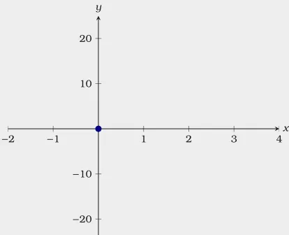
Consider the function
f(x)= 1 (x+1)2
While the lim
x→−1f(x)does not exist, see Figure2.1, something can still be said.
−2 −1.5 −1 −0.5 0.5 1 20
40 60 80 100
x y
Figure 2.1: A plot off(x)= 1
(x+1)2. Definition Iff(x)grows arbitrarily large asx approachesa, we write
lim
x→af(x)=∞
and say that the limit off(x)approaches infinityasx goes toa.
If|f(x)|grows arbitrarily large asx approachesa andf(x)is negative, we write
lim
x→af(x)=−∞
and say that the limit off(x)approaches negative infinityasx goes toa.
On the other hand, if we consider the function
f(x)= 1 (x−1) While we have lim
x→1f(x) , ±∞, we do have one-sided limits, xlim→1+f(x) = ∞and lim
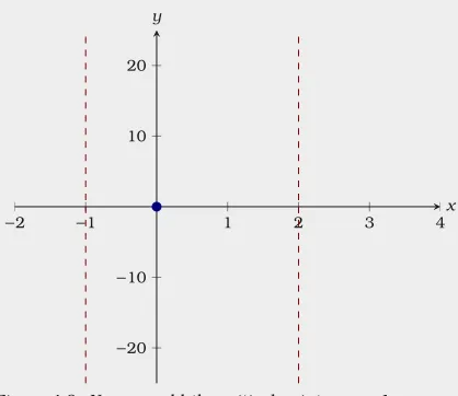
Definition If lim
x→af(x)=±∞, xlim→a+f(x)=±∞, or xlim→a−f(x)=±∞,
then the linex=ais avertical asymptoteoff(x).
Example 2.1.1 Find the vertical asymptotes of
f(x)=x
2
−9x+14
x2−5x+6 .
−1 −0.5 0.5 1 1.5 2
−40 −20 20 40 x y
Figure 2.2: A plot off(x)= 1
x−1.
Solution Start by factoring both the numerator and thedenominator:
x2−9x+14
x2−5x+6 =
(x−2)(x−7) (x−2)(x−3)
Using limits, we must investigate whenx →2andx →3. Write
lim x→2
(x−2)(x−7) (x−2)(x−3)=xlim→2
(x−7) (x−3) = −5
−1 =5.
Now write
lim x→3
(x−2)(x−7) (x−2)(x−3)=xlim→3
(x−7) (x−3) =lim
x→3
−4 x−3. Since lim
x→3+x−3approaches0from the right and the numerator is negative, lim
x→3+f(x)=−∞. Sincexlim→3−x−3approaches0from the left and the numerator
is negative, lim
x→3−f(x)=∞. Hence we have a vertical asymptote atx =3, see
Figure2.3.
1.5 2 2.5 3 3.5 4
−40 −20 20 40 x y
Figure 2.3: A plot off(x)=x
Exercises for Section 2.1
Compute the limits. If a limit does not exist, explain why.
(1) lim x→1−
1 x2−1
➠
(2) lim x→4−
3 x2−2
➠
(3) lim
x→−1+
1+2x x3−1
➠
(4) lim x→3+
x−9 x2−6x+9
➠
(5) lim
x→5
1
(x−5)4
➠
(6) lim
x→−2
1
(x2+3x+2)2
➠
(7) lim
x→0
1
x
x5−cos(x)
➠
(8) lim
x→0+
x−11 sin(x)
➠
(9) Find the vertical asymptotes of
f(x)= x−3
x2+2x−3.
➠
(10) Find the vertical asymptotes of
f(x)=x 2
−x−6 x+4 .
2.2
Limits at Infinity
Consider the function:
f(x)=6x−9
x−1
Asx approaches infinity, it seems likef(x)approaches a specific value. This is a
0.5 1 1.5 2 2.5 3
−10 10 20
x y
Figure 2.4: A plot off(x)=6x−9
x−1.
limit at infinity.
Definition Iff(x)becomes arbitrarily close to a specific valueLby makingx
sufficiently large, we write
lim
x→∞f(x)=L
and we say, thelimit at infinityoff(x)isL.
Iff(x)becomes arbitrarily close to a specific valueLby makingxsufficiently large and negative, we write
lim
x→−∞f(x)=L
and we say, thelimit at negative infinityoff(x)isL.
Example 2.2.1 Compute
lim x→∞
6x−9
x−1 .
Solution Write
lim x→∞
6x−9
x−1 =xlim→∞
6x−9
x−1 1/x
1/x
= lim x→∞
6x x −
9
x x x −
1
x
= lim x→∞
6 1 =6.
Example 2.2.2 Compute
lim x→−∞
x+1 √
x2
Solution In this case we multiply the numerator and denominator by−1/x,
which is a positive number as since x→ −∞, x is a negative number.
lim x→−∞
x+1 √
x2 =xlim→−∞
x+1 √
x2 ·
−1/x −1/x
= lim x→−∞
−1−1/x √
x2/x2
=−1.
Here is a somewhat different example of a limit at infinity. Example 2.2.3 Compute
lim x→∞
sin(7x)
x +4.
5 10 15 20
3.5 4 4.5 5
x y
Figure 2.5: A plot off(x)=sin(7x)
x +4.
Solution We can bound our function
−1/x+4≤sin(7x x)+4≤1/x+4. Since
lim
x→∞−1/x+4=4=xlim→∞1/x+4
we conclude by the Squeeze Theorem, Theorem1.3.5, lim x→∞
sin(7x)
x +4=4.
Definition If
lim
x→∞f(x)=L or xlim→−∞f(x)=L,
Example 2.2.4 Give the horizontal asymptotes of
f(x)=6x−9
x−1
Solution From our previous work, we see that lim
x→∞f(x)=6, and upon further
inspection, we see that lim
x→−∞f(x)=6. Hence the horizontal asymptote of f(x)is
the line y=6.
It is a common misconception that a function cannot cross an asymptote. As the next example shows, a function can cross an asymptote, and in this case this occurs an infinite number of times!
Example 2.2.5 Give a horizontal asymptote of
f(x)=sin(7x)
x +4.
Solution Again from previous work, we see that lim
x→∞f(x)=4. Hence y=4is
a horizontal asymptote of f(x).
We conclude with an infinite limit at infinity. Example 2.2.6 Compute
lim x→∞ln(x)
5 10 15 20
−1 1 2 3 4
x y
Figure 2.6: A plot off(x)=ln(x).
Solution The functionln(x)grows very slowly, and seems like it may have a
horizontal asymptote, see Figure2.6. However, if we consider the definition of the natural log
ln(x)=y ⇔ ey=x
Since we need to raise e to higher and higher values to obtain larger numbers, we see thatln(x)is unbounded, and hence lim
Exercises for Section 2.2
Compute the limits.
(1) lim x→∞ 1 x
➠
(2) lim x→∞ −x √4+x2
➠
(3) lim
x→∞
2x2−x+1 4x2
−3x−1
➠
(4) lim
x→−∞
3x+7 √
x2
➠
(5) lim
x→−∞
2x+7 √
x2+2x−1
➠
(6) lim
x→−∞
x3 −4 3x2+4x−1
➠
(7) lim
x→∞
4
x+π
➠
(8) lim x→∞ cos(x) ln(x)➠
(9) lim x→∞sin x7 √
x
➠
(10) lim
x→∞ 17+
32 x −
(sin(x/2))2 x3
!
➠
(11) Suppose a population of feral cats on a certain college campust years from now is approximated by
p(t)= 1000 5+2e−0.1t.
Approximately how many feral cats are on campus 10 years from now? 50 years from now? 100 years from now? 1000 years from now? What do you notice about the prediction—is this realistic?
➠
(12) The amplitude of an oscillating spring is given by
a(t)=sin(t) t .
2.3
Continuity
Informally, a function is continuous if you can “draw it” without “lifting your pencil.” We need a formal definition.
Definition A functionf iscontinuous at a pointaif lim
x→af(x)=f(a).
2 4 6 8 10
[image:43.792.467.681.309.531.2]1 2 3 4 5 x y
Figure 2.7: A plot of a function with discontinuities atx=4 andx=6.
Example 2.3.1 Find the discontinuities (the values forxwhere a function is not continuous) for the function given in Figure2.7.
Solution From Figure2.7we see thatlim
x→4f(x)does not exist as
lim
x→4−f(x)=1 and xlim→4+f(x)≈3.5
Hencelim
x→4f(x),f(4), and so f(x)is not continuous at x =4.
We also see thatlim
x→6f(x)≈3while f(6)=2. Hencexlim→6f(x),f(6), and so
f(x)is not continuous at x =6.
Building from the definition ofcontinuous at a point, we can now define what it means for a function to becontinuouson an interval.
Definition A functionf is continuous on an intervalif it is continuous at every point in the interval.
In particular, we should note that if a function is not defined on an interval, then itcannotbe continuous on that interval.
−0.2 −0.1 0.1 0.2x
y
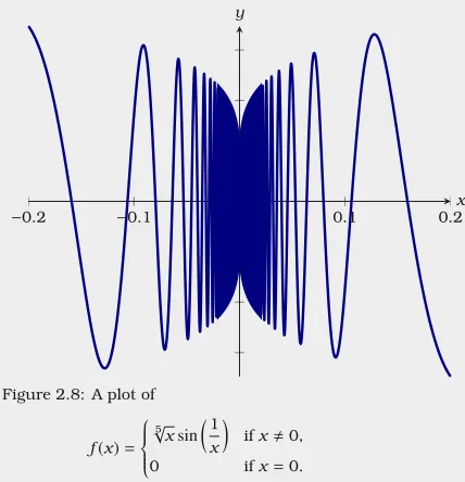
Figure 2.8: A plot of
f(x)= 5 √x sin 1 x
ifx,0,
0 ifx=0. Example 2.3.2 Consider the function
f(x)= 5 √ xsin 1 x
ifx ,0,
0 ifx =0,
Solution Considering f(x), the only issue is when x=0. We must show that
lim
x→0f(x)=0. Note
−|√5x| ≤f(x)≤ |√5x|.
Since
lim x→0−|
5
√
x|=0=lim x→0|
5
√ x|,
we see by the Squeeze Theorem, Theorem1.3.5, thatlim
x→0f(x)=0. Hence f(x)is
continuous.
Here we see how the informal definition of continuity being that you can “draw it” without “lifting your pencil” differs from the formal definition.
We close with a useful theorem about continuous functions:
Theorem 2.3.3 (Intermediate Value Theorem) Iff(x)is a continuous
func-tion for allx in the closed interval[a, b]anddis betweenf(a)andf(b), then
there is a numbercin[a, b]such thatf(c)=d.
The Intermediate Value Theorem is most frequently used whend=0.
For a nice proof of this theorem, see: Walk, Stephen M.The intermediate value theorem is NOT obvious— and I am going to prove it to you. College Math. J. 42 (2011), no. 4, 254–259.
In Figure2.9, we see a geometric interpretation of this theorem.
a c b
f(a) f(c)=d f(b)
x y
Figure 2.9: A geometric interpretation of the Inter-mediate Value Theorem. The functionf(x)is contin-uous on the interval[a, b]. Sincedis in the interval
[f(a), f(b)], there exists a valuecin[a, b]such that
f(c)=d. Example 2.3.4 Explain why the functionf(x)=x3+3x2+x−2 has a root
between 0 and 1.
Solution By Theorem1.3.1,lim
x→af(x)=f(a), for all real values of a, and hence
f is continuous. Since f(0)=−2and f(1)=3, and0is between−2and3, by the Intermediate Value Theorem, Theorem2.3.3, there is a c∈[0,1]such that f(c)=0.
This example also points the way to a simple method for approximating roots.
Example 2.3.5 Approximate a root off(x)=x3+3x2+x−2 to one decimal place.
Solution If we compute f(0.1), f(0.2), and so on, we find that f(0.6) < 0
and f(0.7)>0, so by the Intermediate Value Theorem, f has a root between
that f(0.61) < 0 and f(0.62) > 0, so by the Intermediate Value Theorem, Theorem2.3.3, f(x)has a root between 0.61 and0.62, and the root is 0.6
Exercises for Section 2.3
(1) Consider the function
f(x)=√x−4
Isf(x)continuous at the pointx=4? Isf(x)a continuous function onR?
➠
(2) Consider the function
f(x)= 1
x+3
Isf(x)continuous at the pointx=3? Isf(x)a continuous function onR?
➠
(3) Consider the function
f(x)=
2x−3 ifx <1, 0 ifx≥1.
Isf(x)continuous at the pointx=1? Isf(x)a continuous function onR?
➠
(4) Consider the function
f(x)=
x2
+10x+25
x−5 ifx,5, 10 ifx=5.
Isf(x)continuous at the pointx=5? Isf(x)a continuous function onR?
➠
(5) Consider the function
f(x)=
x2+10x+25
x+5 ifx,−5, 0 ifx=−5.
Isf(x)continuous at the pointx=−5? Isf(x)a continuous function onR?
➠
(6) Determine the interval(s) on which the functionf(x)=x7+3x5−2x+4 is continuous.
➠
(7) Determine the interval(s) on which the functionf(x)=x
2
−2x+1
x+4 is continuous.
➠
(8) Determine the interval(s) on which the functionf(x)= 1
x2−9is continuous.
➠
(9) Approximate a root off(x)=x3−4x2+2x+2 to two decimal places.
➠
3.1
Slopes of Tangent Lines via Limits
Suppose thatf(x)is a function. It is often useful to know how sensitive the value of
f(x)is to small changes inx. To give you a feeling why this is true, consider the following:
• Ifp(t)represents the position of an object with respect to time, the rate of change gives the velocity of the object.
• Ifv(t)represents the velocity of an object with respect to time, the rate of change gives the acceleration of the object.
• The rate of change of a function can help us approximate a complicated function with a simple function.
• The rate of change of a function can be used to help us solve equations that we would not be able to solve via other methods.
The rate of change of a function is the slope of the tangent line. For now, consider the following informal definition of atangent line:
Given a functionf(x), if one can “zoom in” onf(x)sufficiently so thatf(x)seems to be a straight line, then that line is thetangent linetof(x)at the point determined byx.
We illustrate this informal definition with Figure3.1.
x y
Figure 3.1: Given a functionf(x), if one can “zoom in” onf(x)sufficiently so thatf(x)seems to be a straight line, then that line is thetangent lineto
f(x)at the point determined byx.
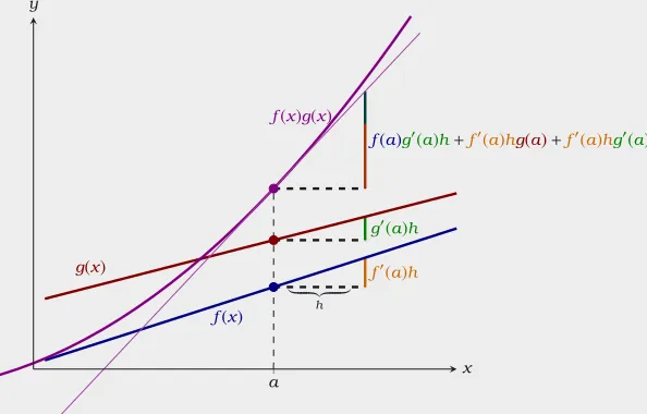
at two points. The slope of any secant line that passes through the points(x, f(x)) and(x+h, f(x+h))is given by
∆y
∆x =
f(x+h)−f(x) (x+h)−x =
f(x+h)−f(x)
h ,
see Figure3.2. This leads to thelimit definition of the derivative:
Definition of the Derivative Thederivativeoff(x)is the function
d
dxf(x)=hlim→0
f(x+h)−f(x)
h .
If this limit does not exist for a given value ofx, thenf(x)is notdifferentiable atx.
x x+h
f(x) f(x+h)
x y
Figure 3.2: Tangent lines can be found as the limit of secant lines. The slope of the tangent line is given by lim
h→0
f(x+h)−f(x)
Definition There are several different notations for the derivative, we’ll mainly use
d
dxf(x)=f
′(x).
If one is working with a function of a variable other thanx, saytwe write
d dtf(t)=f
′(t).
However, ify=f(x), dy
dx,y˙, andDxf(x)are also used.
Now we will give a number of examples, starting with a basic example. Example 3.1.1 Compute
d dx(x
3
+1).
Solution Using the definition of the d