Value of Time Estimation

This is a repository copy of

Value of Time Estimation

_.

White Rose Research Online URL for this paper:

http://eprints.whiterose.ac.uk/2380/

Monograph:

Gunn, F.H. (1987) Value of Time Estimation. Working Paper. Institute of Transport Studies,

University of Leeds , Leeds, UK.

Working Paper 157

[email protected] https://eprints.whiterose.ac.uk/

Reuse

Unless indicated otherwise, fulltext items are protected by copyright with all rights reserved. The copyright exception in section 29 of the Copyright, Designs and Patents Act 1988 allows the making of a single copy solely for the purpose of non-commercial research or private study within the limits of fair dealing. The publisher or other rights-holder may allow further reproduction and re-use of this version - refer to the White Rose Research Online record for this item. Where records identify the publisher as the copyright holder, users can verify any specific terms of use on the publisher’s website.

Takedown

If you consider content in White Rose Research Online to be in breach of UK law, please notify us by

White Rose Research Online

http://eprints.whiterose.ac.uk/

Institute of Transport Studies

University of Leeds

This is an ITS Working Paper produced and published by the University of

Leeds. ITS Working Papers are intended to provide information and encourage

discussion on a topic in advance of formal publication. They represent only the

views of the authors, and do not necessarily reflect the views or approval of the

sponsors.

White Rose Repository URL for this paper:

http://eprints.whiterose.ac.uk/

2380/

Published paper

Gunn, F.H. (1987)

Value of Time Estimation.

_{Institute of Transport Studies,}

University of Leeds, Working Paper 157

UNIVERSITY

OF LEEDS

Institute for Transport Studies

ITS

Working Paper

157

1987

Value of Time Estimation

F

H

GUNN

ABSTRACT

GUNN, Hugh F. (1981) Value of Time Estimation.

Leeds: Univ. Leeds,Inst. Transp. Stud., Work. Pap.

157

The s t a t i s t i c a l a s p e c t s of t h e procedures by which v a l u e s a r e placed on savings i n t r a v e l time, on t h e b a s i s of s t a t e d o r r e v e a l e d preference d a t a , a r e discussed and analysed. Conclusions a r e drawn f o r t h e design of such experiments.

CONTENTS

Chapter

1

The Statistical Problem

1.1 Introduction

1.2 Structure of the Working Paper

2

Basic Assmptions of the Models

2.1

Introduction

2.2

Theory

2.3

Models

2.4

Data

3

Estimation

3.1 Introduction

3.2

Beesleygraph versus Probabilistic

Choice Analysis

3.3

Conclusions

4

Model Validation

4.1

Introduction

4.2

The FPR criterion

4.3

Some comments on the FPR criterion

4.4

Sample Size for the Comparison of Models

4.5

Remarks about FPR1s

and Validation

4.6

Conclusions

5

Efficient Design

5.1

Introduction

5.2

'Optimal Design' and Value-of-Time

5.3

Approximations to the Variance-Covariance

Terms

5.4

Conclusions

6

Transfer Pricing and Revealed Preference

:

a

Comparison of Maximal Efficiency

6.1

Introduction

6.2

Incremental Information in Relative

Magnitude

6.3

Incremental Information in Absolute

Magnitude

-. .

7

Aggregate Methods

7.1 I n t r o d u c t i o n

7.2 The R a t i o s of E l a s t i c i t i e s Approach

8 Conclusions and Recommendations

8.1

I n t r o d u c t i o n 8.2 Sample S i z e

1. THE STATISTICAL PROBLEM.

1.1 Introduction

1.1.1 There a r e two priilcipal approaches t o t h e valuation of t r a v e l t i n e savings:

a ) by t h e a n a l y s i s of t h e outcomes of choices made between numbers of options with d i f f e r i n g , t r a v a l time and cost c h a r a c t e r i s t i c s , and

b ) by t h e a n a l y s i s of direct. estimates of t h e d i f f e r e n c e i n a t t r a c t i v e - ness of p a i r s of options which d i f f e r i n respect of t r a v e l time and c o s t c h a r a c t e r i s t i c s .

When t h e f i r s t approach i s based on observed behaviour, i . e . r e a l options and a c t u a l choices a s revealed by subsequent a c t i o n s , it i s u s u a l l y termed a 'revealed preference' method. When t h e choices a r e hypothetical i n t h e sense of not comitting t h e chooser t o any a c t i o n ,

it

i s u s u a l l y termed a ' s t a t e d preference' approach. The second approach had been

c a l l e d ' t r a n s f e r p r i c i n g ' , although i n p r i n c i p l e t h e measure of difference i n a t t r a c t i v e n e s s could be sought i n terms of t r a v e l time.

We s h a l l not discuss t h e way i n which ' t r a n s f e r p r i c e ' estimates a r e

obtained i n d e t a i l ; put a t i t s simplest, t r a v e l l e r s a r e i n v i t e d t o consider changes i n t h e cost and time a t t r i b u t e s of options, and t o i n d i c a t e

t h e amount of v a r i a t i o n t h a t would be needed t o make t h e options equally a t t r a c t i v e t o them.

1.1.2. The analyses require t h a t t h e l i n k between behaviour and t h e chosen s e t of explanatory v a r i a b l e s , o r t h e l i n k between t h e estimates of t h e d i f f e r e n c e i n a t t r a c t i v e n e s s and t h e s e t of explanatory v a r i a b l e s , be made e x p l i c i t i n parameterised model. Theory suggests only general

The l i m i t a t i o n s of t h e accuracy of t h e model used i n t h e a n a l y s i s t o g e t h e r with t h e amount of data a v a i l a b l e determine t h e accuracy with which t h e parameters i n t h e models can be determined and t h u s t h e accuracy with which values can be a s c r i b e d t o t r a v e l time savings.

1 . 1 . 3 The s t a t i s t i c a l a s p e c t s of t h e problem can be l i s t e d under f i v e headings :

1. How should we draw sample ?

2. How l a r g e must t h e sample be ?

3. How should we estimate t h e parameters i n any model ?

4.

How should we choose between r i v a l models ?

5 .

How can we v a l i d a t e our p r e f e r r e d model ?

These f i v e i s s u e s w i l l a r i s e i n any given survey c o n t e x t , and indeed it w i l l be shown t h a t t h e accuracy with which we can e s t i m a t e model parameters,

f o r given sample s i z e and survey method, v a r i e s from context t o context, so t h a t t h e choice of experimental contkxt i t s e l f should be made with reference t o t h e b a s i c s t a t i s t i c a l problem.

1 . 2 S t r u c t u r e of t h e Working Paper

1.2.1 Throughout most of t h i s paper, we s h a l l assume ourselves i n t h e p o s i t i o n of considering t h e c o l l e c t i o n of disaggregate d a t a s e t s f o r value-of-time estimation. The i n s i g h t s gained on t h e i s s u e of sample s i z e w i l l then a s s i s t i n t h e s c r u t i n y of e x i s t i n g d a t a s e t s , and of course

t h e conclusions reached on model s e l e c t i o n , estimation and v a l i d a t i o n apply equally t o such data. I n p r i n c i p l e , t h e r e s u l t s a l s o apply t o t h e a n a l y s i s of aggregate d a t a s e t s such a s conventional mode s p l i t o r d i s t r i - bution d a t a , where t h e s e can be i n t e r p r e t e d a s t h e outcome o f a d i s c r e t e choice process.

:-

-Some approaches to-value-of--time : r: ~. . .. ~. . . -.

1.2.2. In c o n t r a s t i n g t h e s t a t i s t i c a l p r o p e r t i e s of estimates of model c o - e f f i c i e n t s based on t r a n s f e r - p r i c e measures o f t h e

-

s i z e

of t h e u t i l i t y d i f f e r e n c e with those based only on t h e & o f t h e u t i l i t y d i f f e r e n c e , we s h a l l t a l k of 'maximal' accuracy under f a i r l y s t r o n g hypotheses about t h e accuracy of t h e t r a n s f e r p r i c e . In

p r a c t i c e , t h e degree of success of any t r a n s f e r p r i c e study must depend c r u c i a l l y on t h e s k i l l with which t h e t r a n s f e r p r i c e question i s posed,

a s well a s t h e s u i t a b i l i t y of t h e context f o r such an approach. These probBems p r e s e n t i s s u e s which can only be t a c k l e d by empirical research.

1.2.3. F i n a l l y , we emphasize a t t h e o u t s e t t h a t t h i s paper s e t s out a t h e o r e t i c a l a n a l y s i s of t h e s t a t i s t i c a l a s p e c t s of value o f time estimation. The methods o u t l i n e d below, and t h e formulae given f o r simple models, can be e l a b o r a t e d t o address s p e c i f i c models and contexts

2. BASIC ASSUMPTIONS OF THE MODELS

2.1 Introduction

2.1.1 The concept of 'random u t i l i t y ' allows us t o progress from t h e

u n f a l s i f i a b l e and uninformative a s s e r t i o n t h a t behaviour can be

described i n terms of u t i l i t y maximisation t o t h e s t a g e of p o s t u l a t i n g concrete model forms t o describe and p r e d i c t behaviour and t o e s t a b l i s h

a r a t e a t which time saving can be s u b s t i t u t e d f o r c o s t saving t o

maintain t h e same l e v e l of s a t i s f a c t i o n ( t h e 'compensated marginal value o f t r a v e l time saving' a s defined by Bruzelius, 1979). The device of

specifying t h e u t i l i t y function only up t o a random e r r o r term with unknown variance not only allows us t o proceed with our ( i n e v i t a b l y ) approximate models of behaviour ( a s Daly, 1980, remarks) but a l s o allows us t o measure t h e r e l a t i v e importance o f t h e f a c t o r s omitted f r o m t h e model s p e c i f i c a t i o n i n any p a r t i c u l a r context, by estimating t h a t variance.

.

2.1.2 S p e c i f i c a t i o n o f t h e ' r e p r e s e n t a t i v e ' u t i l i t y f m c t i o n a n d - \

_-

~ '~'*

sh;ecification of t h ~ k a n d o i erro$ term, d$fines a complete model which

can then be'manipulated t o y i e l d both

a

p r o b a b i l i t y d e n s i t y function f o r t h e d i f f e r e n c e betwee

h

t h e u t i l i t i e s o f any two options (and hence a

d i s t r i b u t i o n f o r t h e corresponding Transfer P r i c e estimate, were we t o equate t h a t with t h e u t i l i t y difference) and a corresponding expression f o r t h e p r o b a b i l i t y t h a t

a

p a r t i c u l a r one of t h e options has g r e a t e r u t i l i t y (and hence would be chosen by t h e ' r a t i o n a l decision maker')

than any o t h e r . Both t h e p.d.f. f o r t h e t r a n s f e r p r i c e and t h e p r o b a b i l i t y

t h a t a p a r t i c u l a r option i s chosen a r e defined by t h e 'complete model',

t h e s p e c i f i e d r e p r e s e n t a t i v e u t i l i t y expression and t h e s p e c i f i e d e r r o r term.

Both a r e functions of t h e ( i n i t i a l l y unknown) parameters i n both s p e c i f i c a t i o n s . Standard s t a t i s t i c a l techniques can apply t o e i t h e r

2.2.1 Following t h e now c l a s s i c a l account of t h e theory underlying d i s c r e t e choice ( s e e f o r example i n Williams,

1980)

we can d e s c r i b e

our a n a l y s i s of t h e preferences i n d i c a t e d by p a r t i c u l a r i n d i v i d u a l s over a

f i x e d number of o p t i o n s , N say, a s being based on t h e following p o s t u l a t e s .

1 ) An i n d i v i a u a l drawn a t ranaom from t h e population, with p a r t i c u l a r _- observed c h a r a c t e r i s t i c s , c o n s t r a i n t s and facing a p a r t i c u l a r s e t of options, i s assumed t o be drawn from a subpopulation o f

i n d i v i d u a l s with i d e n t i c a l observed c h a r a c t e r i s t i c s , c o n s t r a i * ~ and options.

2 ) Each of t h e s e i n d i v i d u a l s i s assumed t o . a s s o c i a t e a n e t u t i l i t y with each o p t i o n , U . , i=1,

...,

N

,

and t o s e l e c t t h a t option w i t h

1

t h e highest value of U.

3 ) Individuals within t h e subpopulation with i d e n t i c a l observed c h a r a c t e r i s t i c s , e t c . , a r e assumed t o vary i n respect of some unobserved c h a r a c t e r i s t i c s , i n such a way t h a t t h e net u t i l i t i e s

U1,

...,

UN each vary randomly across t h e subpopulation; t h i s

v a r i a t i o n can be described by a j o i n t d e n s i t y function, f(Ul,

...

UN)

say. Drawing an i n d i v i d u a l a t random from t h e subpopulation r e s u l t s i n observing preferences generated by a v e c t o r of net u t i l i t i e s drawn a t random from t h i s j o i n t d i s t r i b u t i o n .

2.3 Models

2.3.1 We then p o s t u l a t e t h a t t h e nature of t h e v a r i a t i o n o f each Ui

a c r o s s t h e subpopulation o f i n d i v i d u a l s with i d e n t i c a l c h a r a c t e r i s t i c s

can

be represented i n t h e

form

where

Ei,

t h e ' r e p r e s e n t a t i v e u t i l i t y l , i s f i x e d f o r a l l members of t h e subpopulation, and i s a f_unction of observed c h a r a c t e r i s t i c s

Li

describing

i s a v e c t o r of e r r o r terms drawn f r o m e p a r t i c u l a r d i s t r i b u t i o n G say, which i t s e l f contains unknown parameters,& say, and may a l s o be a

1 N

f u n c t i o n of t h e observed c h a r a c t e r i s t i c s

Z

;

..

,

Z

.

We can t h u s w r i t e t h e d i s t r i b u t i o n function o f t h e disturbance terms 1 N

a s G ( S , & , E , - , ~ ) .

The most popular of t h e models t h a t can be generated by s p e c i f i c assumptions about t h e form of

TI

and t h e form of G a r e described i n Gunn e t al (-1980).

2.4

-

Data

2.4.1 Revealed preference d a t a s e t s then c o n s i s t of t h e v e c t o r s o f observed c h a r a c t e r i s t i c s f o r each option a v a i l a b l e , t o g e t h e r with an

i n d i c a t i o n of which option was s e l e c t e d . S t a t e d preference d a t a s e t s can a l s o include a ranking o f preferences extending over a l l o r p a r t of t h e s e t of options. For t r a n s f e r p r i c i n g d a t a s e t s , t h e data r e f e r s t o

comparisons o f p a i r s of options : f o r t r a n s f e r - p r i c e

s t u d i e s (such a s those reported by Hensher, 1976, and Lee and Dalvi, 1969

and 1971) only t h e comparison between t h e o p t i o n a c t u a l l y s e l e c t e d and t h e next-best of t h e a v a i l a b l e options a r e compared, although t h e r e appears t o be no reason ( o t h e r than decreasing c r e d i b i l i t y o f t h e d a t a ) why comparisons should not be made between a l l p o s s i b l e p a i r s of options.

For each p a i r , an estimate of t h e u t i l i t y d i f f e r e n c e i s c o l l e c t e d , t o g e t h e r with t h e two v e c t o r s of observed c h a r a c t e r i s t i c s .

2.4.2 For t h e purposes of i l l u s t r a t i o n , it i s convenient t o consider

a simple case which can be presented g r a p h i c a l l y . Suppose we had a

population of i n d i v i d u a l s with i d e n t i c a l observed c h a r a c t e r i s t i c s , choosing

between two o p t i o n s each o f which was c h a r a c t e r i s e d by only two observed dimensions. We can consider t h i s a s a h i g h l y s i m p l i f i e d r e p r e s e n t a t i o n of t h e choice between two very s i m i l a r modes o f t r a v e l , d i f f e r i n g only i n r e s p e c t o f time and c o s t c h a r a c t e r i s t i c s . For t h e two modes, l e t us

make t h e usual d i s t i n c t i o n between t h e p o s i t i v e u t i l i t y t o be gained a t t h e end of t h e t r i p and t h e - u t i l i t y incurred during t r a v e l i t s e l f , and

j

where t h e termsr) a r e disturbance terms of a magnitude and s i g n u s u a l l y unknown t o t h e modeller, and about which we would usually

only hypothesise t h a t they were drawn from an underlying d i s t r i b u t i o n whose general form could b e - s p e c i f i e d , having u n i t variance.

The n e t u t i l i t y d i f f e r e n c e between t h e o ~ t i o n s

-

i s then eq. -

3

j l

-

j 2 j 2

j

-

u j )

=

-8 _{( Z Zl )}

-

_B2

_(z?

-

_{Z2 ) +}

(4

-

_o;)

C U 1 2 1 1

...

( 3 )

and a s u s u a l , we would assume t h a t mode 1 would be s e l e c t e d if U were

1

l a r g e r than U2, and U only s e l e c t e d if U were smaller t h a n

U

2 1 2'

(We s h a l l ignore t h e p o s s i b i l i t y of k q u a l i t y : )

2.4.3. For each i n d i v i d u a l , we can p l o t a p o s i t i o n on a ( ~ e e s l e ~ - ) graph with axes (z?

-

z?) and

(zF

-

z j 2 )

corresponding t o t h e n e t

2

d i f f e r e n c e i n observed c h a r a c t e r i s t i c s i n t h e o p t i o n s confronting t h e

i n d i v i d u a l . Let us assume t h a t

(z?

-

z?)

r e p r e s e n t s a d i f f e r e n c e i n journey times and denote t h a t a x i s by AT. S i m i l a r l y , l e t ( z F -

zF)

denote d i f f e r e n c e i n c o s t s , and denote t h a t a x i s by AC.

Working Paper

6

h a s d e s c r i b e a t h e e s s e n t i a l indeterminacy i n t h e u n i t

system a p p r o p r i a t e f o r such expressions, and we have seen t h a t , providing we t a k e c a r e t o make c o n s i s t e n t adjustments throughout, we can work

i n any

u n i t

we please. For example, i f we choose t o s e t $ t o u n i t y , l e a v i n g 8 ₂ a s a parameter t o be estimated, we must a l s o acknowledge t h e need t o e s t i m a t e t h e s c a l e parameter i n t h e d i s t r i b u t i o n f u n c t i o n f o r

t h e disturbance term. (The more usual approach i s t o s t a n d a r d i s e t h a t s c a l e parameter t o unity and express t h e problem a s one of e s t i m a t i n g

both and 02: i n p r a c t i c e , of course, t h i s amounts t o e x a c t l y t h e same t h i n g ) . To i l l u s t r a t e t h e r e l a t i o n s h i p between t h e . t r a n s f e r p r i c e and revealed preference approach, it i s usef'ul t o work throughout i n money u n i t s , s o l e t u s r e w r i t e e q 3 a s

/

2

Where

=

B;!

and vm E =

l / e l

I n t h i s fonn

3

v a r E must now be estimated.

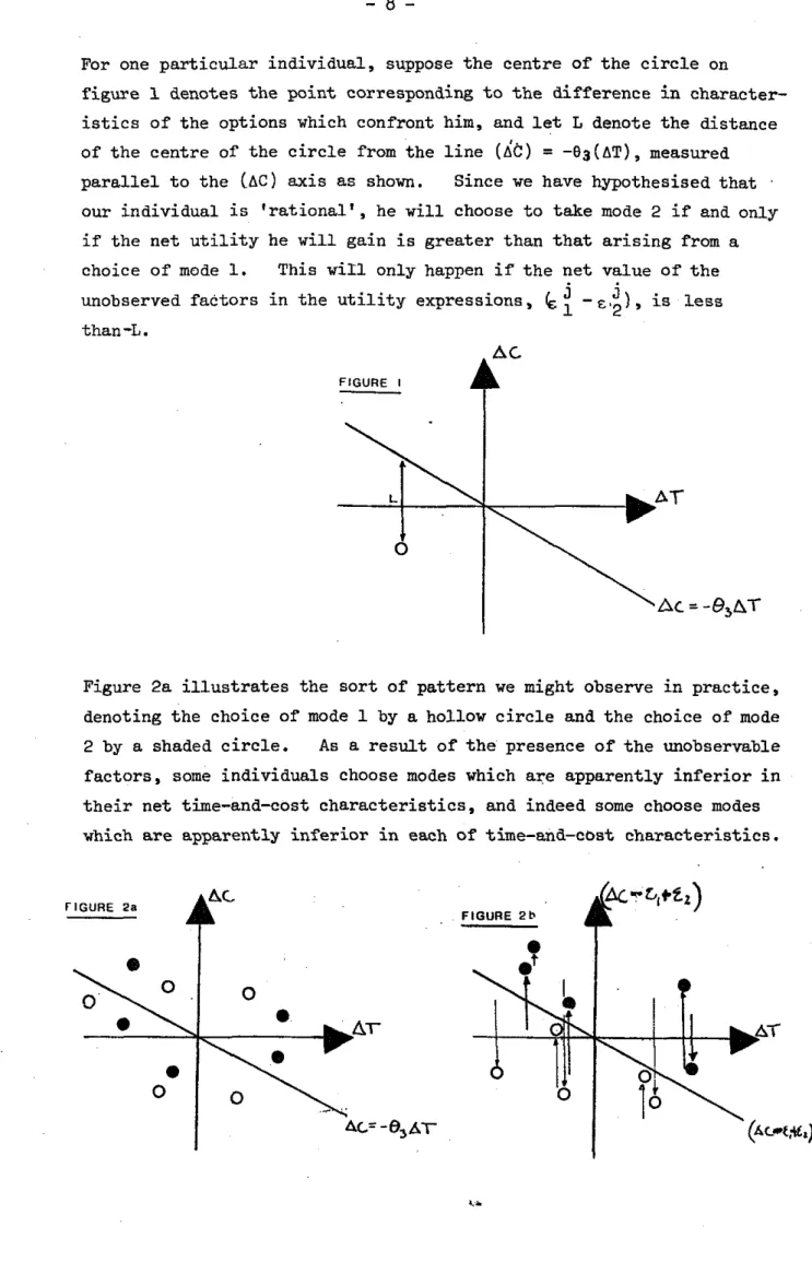
For one particular individual, suppose the centre of the circle on

figure

1

denotes the point corresponding to the difference in character-

istics of the options which confront him, and let

L

denote the distance

of the centre of the circle from the line

( L C )

=

-e3(AT),

measured parallel to the ( A C ) axis as shown. Since we have hypothesised that

our individual is 'rational', he will choose to take mode 2 if and only

if the net utility he will gain is greater than that arising from a

choice of mode 1. This will only happen if the net value of the

j

unobserved faCtors in the utility expressions,

6

-

E?), is less

2

than

-L.

Figure 2a illustrates the sort of pattern we might observe in practice,

denoting the choice of mode 1 by a hollow circle and the choice of mode

2 by a shaded circle. As a result of the presence ofthe unobservable

factors, some individuals choose modes which are apparently inferior in

their net time-and-cost characteristics, and indeed some choose modes

which are apparently inferior in each of time-and-cbst characteristics.

FIGURE 2a

Now l e t u s suppose t h a t t h e n e t e f f e c t of t h e unobservables ( E ' - € . )

1 2

could be determined t h a t weknew6 and t h a t we could r e p l o t each

-

3'

-

i n d i v i d u a l on a graph with axes AT and ( A C- E +E ). Figure 2b

1 2

i l l u s t r a t e s t h e expected r e s u l t : every i n d i v i d u a l i s now seen t o be making a rabional choice.

2.4.4 The t r a n s f e r p r i c e questions described i n Working Paper

6

a r e intended t o - d i s c o v e r t h e net- u t i l i t y d i f f e r e n c e between t h e options

f o r each i n d i v i d u a l ; i n f i g u r e 2b, t h i s would correspond t o t h e d i s t a n c e from t h e ' l o c a t i o n ' of each i n d i v i d u a l t o t h e l i n e '

E +.E )=--0 AT measured p a r a l l e l t o t h e (AC

-

el + E ~ ) a x i s .

1 2 3

It i s easy t o s e e t h a t I F we d i d have a measure o f ( E ~ - E ~ ) , AND t h e

t r a n s f e r p r i c e d a t a did t r u l y represent t h e n e t d i f f e r e n c e i n u t i l i t y between t h e o p t i o n s , we could

r e p l o t t h e p o i n t s corresponding FIGURE 3 e

t o each i n d i v i d u a l on a graph

with axes A T and ( AC 7

+

_E~

-

TE),

and t h a t we would then f i n d t h a t

a l l t h e p o i n t s l a y on t h e l i n e (AC

-

E~ f E~

-

TP)=-8 AT, a s

3 i l l u s t r a t e d i n f i g u r e 3a.

FIGURE 36

%

I n p r a c t i c e , we only know AT and AC-TP P l o t t i n g i n d i v i d u a l s ' l o c a t i o n s on t h e s e axes produces a s e t of p o i n t s s c a t t e r e d

about t h e (AC-TP)=-8 AT l i n e , a s on

3

Figure 3b, where t h e displacement from t h e l i n e i s j u s t t h a t which d i s t i n g u i s h e s

'

d

C

-

'

'

)

r

-

'

>

~

r

f i g u r e 2b from f i g u r e 2a,

i . e .

t h e net

.(

e

e f f e c t o f t h e unobservables.

The estimation of t h e slope of t h e l i n e t h e n becomes a m a t t e r f o r

s t a t i s t i c a l r e s o l u t i o n , given t h e e r r o r d i s t r i b u t i o n s o f t h e s e

unobservables. For example if they were a l l normally d i s t r i b u t e d with constant variance, we would f i t t h e f a m i l i a r ' l e a s t square' r e g r e s s i o n

l i n e .

2.4.5 I n p r a c t i c e , of course, it i s d e s i r a b l e t o allow f o r t h e

p o s s i b i l i t y t h a t t h e t r a n s f e r p r i c e d a t a does not g i v e an exact measure of t h e u t i l i t y d i f f e r e n c e between t h e o p t i o n s , but i s i t s e l f s u b j e c t t o c e r t a i n e r r o r s . This p o s s i b i l i t y i s discussed by Daly (1979) who demonstrates t h a t simple s o l u t i o n s a r e a v a i l a b l e f o r conveniently chosen

e r r o r d i s t r i b u t i o n s . Daly* has a l s o noted t h a t an elegant d i s t i n c t i o n can be made between t h e d i s t r i b u t i o n s of t r a n s f e r p r i c e s i n t h e context

of choices a c t u a l l y made and t h o s e f o r h y p o t h e t i c a l options and contexts, i n t h a t t h e former can be r e s t r i c t e d t o t a k e only

p o s i t i v e values. Thus, a t t h e expense of some e x t r a complexity, we can ensure t h a t t h e t r a n s f e r p r i c e question can o n l y

add

t o our information

if we a c t u a l l y know t h e outcome of t h e choice.

*

p r i v a t e communication.

3. ESTIMATION

3.1 Introduction

3.1.1 The relative advantages of the various methods by which

probabilistic choice models can be estimated are by now well known

(see for example Stopher and Meyburg,

1976)

and the analysis of transfer

price data calls only for the straightforward application of regression

methods (Daly

19781.

We shall not discuss these here.

3.1.2 Instead, in recognition of the historical importance of the

'Beesleygraph' approach in connection with the analysis of binary choice

data for value of time measurement, the interest there is in the

connection between this method and the more recent probabilistic choice

analyses, and the importance of the related issues of use of data, we

shall use this section to pursue the graphical illustration of the

previous section in demonstration of the essential differences between

the methods.

3.2. Beesleygraph versus Probabilistic Choice Analysis.

3.2.1 The 'Beesleygraph' technique can be simply illustrated as

follows; obtain a sample of outcomes of choices between two options

differing in respect of time and cost characteristics, and plot these on

net time cost, net money cost axes as on figure ha, distinguishing as

mode 1 was s e l e c t e d and those points a t which mode 2 was selected. The problem i s then t o f i n d t h a t s t n a i g h t l i n e drawn through t h e o r i g i n which minimises t h e number of p o i n t s a t which t h e mode chosen i s

apparently i n c o n s i s t e n t with r a t i o n a l behaviour i n terms of time and c o s t alone.

The d a t a p o i n t s i n t h e f i r s t and t h i r d quadrants a r e redundant f o r t h i s

a n a l y s i s ; were t r a d i n g t o occur on time and c o s t alone, mode 2 should always be chosen by those i n t h e f i r s t quadrant and mode 1 by those i n t h e t h i r d quadrant, (one mode being b e t t e r than t h e o t h e r i n ' a l l ' r e s p e c t s i n t h e s e a r e a s ) .

3.2.2 Figure 4b i l l u s t r a t e s t h e process with a l i n e drawn which r e s u l t s i n only two apparently ' i n c o n s i s t e n t ' observations; 'consistency' would r e q u i r e t h a t a l l decisions c h a r a c t e r i s e d a s p o i n t s p l o t t e d above t h e l i n e

l e d t o mode 2 being s e l e c t e d , s i n c e i n t h a t a r e a we have AC > 8 AT

3

o r (c1-c2) > O 3 (T1-T2) i . e . t h e value of t h e time saving o f f e r e d by mode 2 outweighs i t s e x t r a c o s t (above t h e l i n e i n quadrant 4 ) o r t h e c o s t saving offered by mode 2 outweighs t h e e x t r a time taken (above t h e

l i n e i n quadrant 2 ) . S i m i l a r l y , a l l 'decision p o i n t s ' below t h e l i n e should r e s u l t i n t h e s e l e c t i o n o f mode 1.

3.2.3 Now l e t us consider t h e corresponding a n a l y s i s provided by, f o r example, l o g i t a n a l y s i s , using e x a c t l y t h e same model of n e t u t i l i t y .

The p r o b a b i l i s t i c choice a n a l y s i s s u p p l i e s , f o r every p o i n t on t h e decision plane, a p r o b a b i l i t y t h a t mode 1 would be s e l e c t e d (and o f course t h e

p r o b a b i l i t y t h a t mode 2 would be s e l e c t e d i s t h u s defined a t t h e same time). We can i l l u s t r a t e t h e end r e s u l t

by drawing a s e r i e s of i s o -

probability-choosemode-1 l i n e s one t h e decision plane, a s i n f i g u r e

5.

It can now be seen q u i t e v i v i d l y t h a t t h e d a t a must supply an e x t r a piece of

information, f o r t h e model

r e q u i r e s not only an o r i e n t a t i o n f o r t h e i s o - p r o b a b i l i t y l i n e s , but a r a t e of change a l s o

P C rob( mode t I

For example, in figures 6a and b we have iso-probability lines

corresponding to differences in orientation(va1ue-of-time) but not

rate of change, and in figures 7a and b we show differences

in

rate-

of-change for lines with the same orientation.

P.

' '3 A c

'..

FIGURE 6a

9

' '9

. . We are free to choose a

system of units for our utility expressions, provided that we remember

that the dispersion of the random element must then be made parametric.

The rate-of-change of the iso-probability lines is determined by just

this dispersion. The requirement that the data determines this rate-of-

change reflects our implicit choice of a particular unit system (money)

3.3. Conclusions

3.3.1 The example given above i l l u s t r a t e s e x a c t l y why t h e p r o b a b i l i s t i c choice models a r e p o t e n t i a l l y more powerful i n t h e i r use of data than t h e 'Beesleygraph' approach. The evidence f o r t h e o r i e n t a t i o n of t h e

e q u i p r o b a b i l i t y l i n e s i s taken from ALL t h e d a t a , r e g a r d l e s s of i t s

l o c a t i o n on t h e plane. On t h e o t h e r hand, it i s a l s o c l e a r t h a t

' p o t e n t i a l power' and ' l a c k of robustness' w i l l go hand i n hand, and t h a t t h e p r o b a b i l i s t i c choice models w i l l be more s e n s i t i v e t o miscoded d a t a

p o i n t s , o r s e c t i o n s of t h e data t o which t h e model does not apply. Ignoring t h e evidence from observations i n quadrants 1 and 3, a s i s i n e v i t a b l e with t h e 'Beesleygraph' approach a s o u t l i n e d and indeed a s has been done i n t h e p a s t i n s p e c i f i c t r a n s f e r p r i c e experiments ( s e e Lee and Dalvi, 1969)

-

does r e s u l t i n t h e l o s s of information t h a t could improve

estimates of c o - e f f i c i e n t s i n p r o b a b i l i s t i c choice models, o r i n t r a n s f e r -

p r i c e experiments, ( a t l e a s t if t h e model and d a t a a r e both c o r r e c t ) .

However, such an omission should not b i a s t h e r e s u l t s , merely reduce t h e i r p r e c i s i o n .

3.3.2 The 'Beesleygraph' approach i l l u s t r a t e d h e r e i s a s p e c i f i c , highly s i m p l i f i e d a p p l i c a t i o n of t h e 'Score Maximisation' technique

4.

MODEL VALIDATION

4 . 1

I n t r o d u c t i o n

4.1.1

The general t a s k of model a p p r a i s a l can be considered under two headings. F i r s t l y , t h e r e i s t h e i s s u e of t h e i n t e r n a l consistency of t h e complete model with t h e d a t a from which it has been estimated. This aspect of a?pi-aisal includes t h e well-known t e s t s of s i g n i f i c a n c e

and examinations of r e s i d u a l s from standard s t a t i s t i c a l theory; f o r disaggregate choice models, t h e various t e s t s t h a t a r e commonly used a r e

l i s t e d i n Gunn e t a 1 (1980). To t h i s l i s t we would now add t h e Lagrangian M u l t i p l i e r t e s t s and t h e range o f ' o v e r f i t t i n g ' t e s t s

described by Horowitz (1980). The second i s s u e concerns t h e performance of t h e f i t t e d models, and t h e d e s c r i p t i o n of behaviour and values t h a t

t h e s e embody, i n t h e p r e d i c t i o n of choice f o r d a t a s e t s o t h e r than t h a t

from which t h e model has been estimated. T h i s we s h a l l c a l l ' v a l i d a t i o n ' .

4.1.2 I n t h i s s e c t i o n , we s h a l l discuss t h e second of t h e s e i s s u e s

i n t h e context of one p a r t i c u l a r t e s t described by F o e r s t e r (1979). I n p a r t i c u l a r , we a r e i n t e r e s t e d i n t h e question o f t h e amount o f d a t a t h a t i s necessary t o ' v a l i d a t e ' a model. A s e p a r a t e question concerns t h e

-

s o r t of d a t a t h a t should be used f o r v a l i d a t i o n . Most f r e q u e n t l y , t h e v a l i d a t i o n data s e t i s a c t u a l l y a randomly s e l e c t e d subsample o f

t h e estimation data s e t ; c e r t a i n l y a v a l i d a t i o n procedure based on such a p a r t i t i o n i n g of t h e d a t a w i l l guard a g a i n s t some of t h e dangers of model m i s s p e c i f i c a t i o n . However, i n many c a s e s it w i l l be c l e a r from t h e

purpose f o r which t h e model has been developed t h a t t h e r e i s a p a r t i c u l a r s o r t of context i n which t h e model should be v a l i d a t e d . For example,

if t h e model i s derived from data from one s e t of geographical a r e a s f o r

g e n e r a l a p p l i c a t i o n i n o t h e r a r e a s ,

it

should be t e s t e d s p e c i f i c a l l y f o r i t s performance i n a sample of such o t h e r areas. S i m i l a r l y , a f o r e c a s t i n g

model should be t e s t e d f o r i t s performance i n o t h e r time periods.

about 'values-of-time' from revealed preference d a t a i s a l l CONDITIONAL on t h e adequacy o f t h e model used t o represent behaviour. We should not underestimate t h e importance of e s t a b l i s h i n g t h e adequacy of t h a t

r e p r e s e n t a t i o n .

4.2. The FPR C r i t e r i o n f o r Model Validation and f o r Model Comparison Using Validation Data S e t s

4.2.1 A disaggregate model s p e c i f i e s a s e t of p r o b a b i l i t i e s a t t a c h i n g t o each of a number of o p t i o n s a v a i l a b l e t o an i n d i v i d u a l . The option a s s o c i a t e d with t h e maximum of t h e s e p r o b a b i l t i e s w i l l be deemed t h e i n d i v i d u a l ' s ' f i r s t p r e f e r e n c e ' . I n a p p l i c a t i o n t o a v a l i d a t i o n d a t a s e t , t h e model may o r may not i n d i c a t e t h a t t h e option a c t u a l l y s e l e c t e d was t h e ' f i r s t preference' f o r t h e i n d i v i d u a l . I f it does, t h i s i s

deemed t o be a ' f i r s t preference recovery'.

Naturally we would not expect a l l i n d i v i d u a l s t o s e l e c t t h e i r 'maximum p r o b a b i l i t y ' o p t i o n i f t h e model were a b s o l u t e l y c o r r e c t ( u n l e s s of course t h e model was specifying p r o b a b i l i t i e s of 1 f o r t h a t option and thus

0 f o r a l l o t h e r s ) : In g e n e r a l , t h e expected number of FPR's w i l l depend on t h e a c t u a l s i z e s of t h e maximum p r o b a b i l i t i e s , assuming a c o r r e c t l y s p e c i f i e d model. This i s discussed l a t e r ; f i r s t we s h a l l consider t h e comparison of two competing models.

4.2.2 Two d i f f e r e n t models may be compared i n respect of t h e i r FPR's by a method described by F o e r s t e r (1979), due o r i g i n a l l y t o McNemar and

g e n e r a l i s e d by Cochran (1950) t o apply t o an a r b i t r a r y number of models o r weighted averages of models. Only t h e simple case of two model comparisons w i l l be considered here.

Consider a 2x2 t a b l e l a y o u t a s shown i n f i g .

8;

f o r each i n d i v i d u a l i n t h e v a l i d a t i o n sample, a s e t of probabiliities o f choosing each o p t i o n i s

c a l c u l a t e d f o r each o f t h e two models under i n v e s t i g a t i o n . The i n d i v i d u a l i s assigned t o one of t h e c e l l s of t h e t a b l e according t o t h e r u l e s :

a s s i g n t o c e l l ( 1 , l ) i f t h e a c t u a l option chosen i s not t h e 'maximum p r o b a b i l i t y ' option f o r e i t h e r model;

a s s i g n t o c c l l ( 2 , l ) i f t h e a c t u a l o p t i o n chosen i s t h e mnx. prob. o p t i o n f o r model 1 b u t not f o r model 2 ;

a s s i g n t o c c l l ( 2 , 2 ) i f chosen o p t i o n i s t h e max. prob. o p t i o n f o r each model.

FIGURE 8

n . ₁₁ = no. indlvlduals assrgned ro cel 1 i

,

i 1 noFPR F F R

hGx?-,

4.2.3 T h i s s o r t o f contingency t a b l e l a y o u t i s most f a m i l i a r i n t h e c o n t e x t of a n u l l h y p o t h e s i s o f independence o f row and column c l a s s i -

2 .

f i c a t i o n s , which i s t e s t e d with t h e

x

d i s t r i b u t e d s t a t i s t i c

2

~ ~ = z ( ~ ~ ~ - ~ t ~That h y p o t h e s i s ) i s n o t a p p r o p r i a t e i n t h i s

1, .ell

c a s e , q u l t e a p a r t from b e i n g h i g h l y i m p l a u s i b l e f o r any s e n s i b l e p a i r of models (which should be s p e c i f y i n g broarllx s i m i l a r c h o i c e

p r o b a b i l i t i e s , t h u s c o n c e n t r a t i n g t h e d a t a i n t h e ( 1 , l ) and ( 2 , 2 ) c e l l s ) . R a t h e r , we a r e i n t e r e s t e d i n t h e n u l l h y p o t h e s i s t h a t t h e p r o b a b i l i t i e s w i t h which i n d i v i d u a l s f a l l i n t o t h e ( 2 , l ) and ( 1 , 2 )

c e l l s a r e e q u a l , f o r i n t h a t c a s e t h e i m p l i c a t i o n i s t h a t t h e two models a r e e q u i v a l e n t i n terms o f expected number of FPR's. Wc can t e s t t h i s h y p o t h e s i s by c o n s i d e r i n g t h e e n t r i e s i n t h e ( 1 , 2 ) and ( 2 , l ) c e l l s a l o n e . On t h e n u l l h y p o t h e s i s o u t l i n e d , ( a f t e r McNemar), t h e s t a t i s t i c Q,

Q = (n12- 1'2~",2+021))2 ("21

-112'"12+"21))2

+

1 ~ 2 1 n , 2 + n 2 ~ ) 112(n12+ "211 i s

x2

d i s t r i b o t c d w i t h 7 d.f.

- -

2

With some e a s y m a n i p u l a t i o n , we can show t h a t

=

1 n 1 2 - v l 1 ( " 1 2

+

"21 1

4.2.4 Thus, a t e s t o f t h e ' e q u i v a l e n c e ' o f t h e two models, - i n t e r m s o f 1 1 1 i s given by computirlg Q and comparinp, t h e r e s u l t w i t 1 1

x

2

-

1

2 1.C Q i s n o t l a r g e r t h a n t h e a p p r o p r i a t e chosen c r i t i c a l v a l u e of

_{x 1}

(3.85 f o r t h e u s u a l

95%

confidence l e v e l ) we conclude t h n t t h e models a r e equivalent i n t h e s e t e r m s .

I

-

ln12-"21-112

Cochrnn n l s o g i v e s a s t a t i s t i c ' c o r r e c t e d f o r c o n t i n u i t y ' , o -

"I:+ "21

Thus, given n

1 2 and nZ1, we can simply c o n s u l t t a b u l a t e d v a l u e s of t h e s i g n t e s t ( f o r example s e e Crow, Davis and Maxwell, Table

9 )

t o t e s t t h e h y p o t h e s i s t h a t t h e p r o b a b i l i t i e s o f an i n d i v i d u a l b e i n g a s s i g n e d t o t h e

( 1 , 2 ) c e l l , and t o t h e ( 2 , l ) c e l l , a r e equal.

4 . 3 Some comments on t h e FPR C r i t e r i o n

4.3.1 The FPR c r i t e r i o n h a s some i n t u i t i v e a p p e a l ; it i s easy t o c a l c u l a t e and h a s an obvious s o r t o f connection w i t h model performance. However, it should be s t r e s s e d t h a t it i s n o t i n i t s e l f an unambiguous i n d i c a t o r of model r e l i a b i l i t y ; t o o many FPRs should l e a d t o r e j e c t i n g t h e model as w e l l as t o o few. This i s d i s c u s s e d more f u l l y l a t e r . A second p o i n t i s t h a t , even if t h e t o t a l numbers of FPRs a r e a c c e p t a b l e , a t e s t which weights each c o r r e c t p r e d i c t i o n e q u a l l y w i l l not be

s u i t a b l e f o r circumstances where some o p t i o n s a r e more important than o t h e r s . For example, a mode-split model might s p e c i f y s e v e r a l modes b u t be p a r t i c u l a r l y i n t e r e s t i n g i n r e s p e c t o f i t s p r e d i c t i o n s o f

patronage o f a minor mode such a s car-pooling. We would n o t t h e n judge two r i v a l models e q u i v a l e n t even i f t h e y had e x a c t l y t h e same number of FPRs, i f one model g o t t h e car-pooling patronage e n t i r e l y 'wrong', and all o t h e r modes correspondingly s l i g h t l y more ' r i g h t ' , t h a n a r i v a l model which performed adequately f o r all modes, i n c l u d i n g car-pooling.

4.3.2 The l a t t e r p o i n t i s l i n k e d t o t h e choice o f sample f o r t h e v a l i d a t i o n e x e r c i s e . This r e q u i r e s t o be chosen randomly from t h e p o p u l a t i o n b e i n g modelled, i n o r d e r t o allow t h e d e s i r e d i n f e r e n c e about t h e g e n e r a l s u i t a b i l i t y of t h e models i n t h i s p o p u l a t i o n ; however, i f some o p t i o n s a r e more ' i m p o r t a n t ' t h a n o t h e r s , it seems c l e a r t h a t t h i s importance should b e r e f l e c t e d somehow i n t h e

composition of t h e v a l i d a t i o n sample. This q u e s t i o n i s n o t e x p l o r e d h e r e , b u t i n p a s s i n g it can b e seen t h a t t h e need f o r a v a l i d a t i o n p r o c e s s emphasises t h e importance of c o n s i d e r a t i o n s o f sample s i z e and d e s i g n , e s p e c i a l l y i f b o t h e s t i m a t i o n and v a l i d a t i o n d a t a i s g a t h e r e d

at t h e same time. The accuracy of one s t a g e may t h e r e a f t e r only b e i n c r e a s e d at t h e expense o f t h e accuracy o f t h e o t h e r .

4.4

Sample s i z e f o r t h e comparison of models by t h e Q s t a t i s t i c

4.4.1

Given t h e procedure o u t l i n e d above, based on t h e number of FPRs, we can choose whichever l e v e l o f confidence seems a p p r o p r i a t e f o r t h e a s s e r t i o n t h a t t h e two models under comparison d i f f e r i n r e s p e d t of expected number o f FPRs. We t h u s have c o n t r o l o v e r t h c

f r a c t i o n of times t h a t we w i l l i n c o r r e c t l y a s s e r t a d i f f e r e n c e between s i m i l a r models. As usual, t h e aim of s e l e c t i n g a p a r t i c u l a r sample s i z e i s t o ensure a corresponding c o n t r o l over t h e proportion of times we w i l l make t h e other s o r t of e r r o r , namely i n c o r r e c t l y concluding t h a t t h e r e i s no d i f f e r e n c e between d i f f e r e n t models.

4.4.2 The a c t u a l c a l c u l a t i o n of t h e p r o b a b i l i t y of an e r r o r o f t h e second kind depends on t h e exact difference between t h e models, which of course, w i l l not be known a t t h e o u t s e t . One way around t h i s

problem i s a v a i l a b l e , i f we a r e able t o decide on a minimum d i f f e r e n c e t h s t we should l i k e t o be a b l e t o d e t e c t . If we t h e n c a l c u l a t e t h e

sample s i z e needed t o reduce t h e chance of e r r o r s of t h e second kind t o an acceptable l e v e l f o r models which d i f f e r by e x a c t l y t h i s minimum amount, then we have ensured t h a t t h e r e w i l l be even l e s s chance of such an e r r o r f o r discriminating between models which d i f f e r by more than t h e minimum of i n t e r e s t .

4.4.3 The a c t u a l s i z e of t h e minimum d i f f e r e n c e t h a t we should aim t o d e t e c t w i l l vary from a p p l i c a t i o n t o a p p l i c a t i o n , and may i n many c a s e s be a m a t t e r f o r judgement r a t h e r than f o r hard and f a s t r u l e s , although it may be p o s s i b l e t o develop a decision-theoretic approach f o r problems i n which t h e ' c o s t ' of wrong p r e d i c t i o n s can be estimated. For t h e purpose o f i l l u s t r a t i o n , t a b l e 1 l i s t s t h e p r o b a b i l i t i e s of an e r r o r of. t h e second kind corresponding t o various sample s i z e s when t h e c r i t e r i a Q and Q' a r e used t o a s s e s s t h e s t a t i s t i c a l s i g n i f i c a n c e of t h e d i f f e r e n c e between FPRs of two models, f o r t h e p a r t i c u l a r c a s e when P r ( 1 , 2 ) = 0.05 and P r ( 2 , l ) = 0.00. ( P r ( i , j ) denotes t h e

p r o b a b i l i t y t h a t an i n d i v i d u a l drawn a t random from t h e v a l i d a t i o n d a t a s e t w i l l be assigned t o c e l l ( i , j ) i n t h e t a b l e i n f i g . 1 . ) This p a r t i c u l a r case corresponds t o two models such t h a t , on average, model 2 produces

5

e x t r a FPHs per 100 individuals modelled a s compared t o model 1. For t h e purposes of t h e t e s t , it does not m a t t e r whether t h i s a r i s e s a s a r e s u l t of model 1 having 0% FPRs and model 2 10% FPR, o r model 1 80% and model 2 90% FPRs.

4.4.4

For t h i s case, n w i l l always be 0, so Q simply becomes n

21 12'

and Q' becomes (n12-112

.

If we a r e ensuring 95% confidence t h a t any

n _{1 2}

models, we w i l l . be comparing Q nnd 0.' r e s p e c t i v e l y with t h c n p p r o p r i a t c 2

v a l u e of X1

,

namely 3.85. Thus, i f we c o n s i d c r t h e t e s t based on Q

f o r example, t h e p r o b a b i l i t y o f an e r r o r of t h e s e c o n d k i n d , namely a c c e p t i n g t h e n u l l h y p o t h e s i s o f no d i f f e r e n c e between t h e two models, i s t h e p r o b a b i l i t y o f t h r e e o r f e v e r i n d i v i d u a l s heing'c1a:;:;ified t o t h e ( 1 , 2 ) c e l l . For any given sample s i z e , n s a y , t h e p r o b a b i l i t y

t h a t r i n d i v i d u a l s w i l l bc a s s i g n e d t o t h e (1,') c e l l i s simply t h e n

Binomial p r o b a b i l i t y c, P'(l-p)n-r, where p d e n o t e s t h e p r o b a b i l i t y o f an i n d i v i d u a l chosen a t random b e i n g a s s i g n e d t o t h e ( l , 2 ) c e l l . Civcn n , und t a k i n g p = 0 . 0 5 , we can c n l c u l r r t e t h c p r o t ~ n \ ~ i l i t i e o o f 0, 1, 2 and 3 i n d i v i d u a l s b e i n g a s s i g n e d , and S~LTI t h e s e t o ir,ive t h e

t o t a l p r o b a b i l i t y of a c c e p t i n g t h e n u l l hypothesi:;, which i s , i n t h i s c a s e , an e r r o r o f t h e second kind. The c a l c u l a t i o n f o r C),' i s

s i m i l a r , e x c e p t t h a t we must al.so add t h e p r o b a l ~ i l i . t i e s o f e x a c t l y

4

and e x a c t l y

5

i n d i v i d u a l s i n t h e ( 1 , 2 ) c e l l , s i n c e t h e nu1.l h y p o t h e s i s i s r e j e c t e d o n l y f o r n12

2

6.

11 .I4

.

5

Q' i s n more ' c o n s e r v n t i v e ' s t a t i s t i c 1:hm

9,

i n t h e !;cr!!;c

t h a t i t r e q u i r e s s t r o n g e r proof c f any d i f f e r e n c e betwee11 n:odel.s. Correspondingly, it i s more prone t o make e r r o r s o f t h c second k i n d ,

f ~ i i l i n e , t o de.teet d i f f c r c n e c s when t h e y do o c c u r . It i s c l c a r from tab1.e 1 t h a t t h e r e q u i r e d v a l i d a t i o n s a n ~ p l a s i z e rieeds t o be r e l a t i v e 1 . y

q u i t e l a r g e , g i v e n t h a t t h e e s t i m a t i o n d a t a s e t s a r e u s u a l l y only a few hundred d a t a p o i n t s , t o a l l o w .us t o d i s c r i m i n a . t e between t h e two modcls under c o n s i d e r a t i o n with any degree o f c e r t a i n t y .

'Pablc 1. Probabilities o f an e r r o r o f t h e second kind f o r ~ is;unnlc v ~ s i z e , and s t u t e d t e s t , t e s t s i z e , and models a:; defin?&

Sample s i z e

50 100

150

200 250

~ r ( e r r o r 11)

Q

.76

.26

.05

The method o u t l i n e d h e r e can be extended t o i n d i c a t e recluircd

v a l i d a t i o n sample s i z e s f o r o t h e r l e v e l s o f minimum d i f f e r e n c e , i.ncluding c a s c s where b o t h (1.2) a n d ( 2 , l ) c e l l s have non-zero p r o b a b i l i t i c : ; .

5

Remarks about FPRs and ' v a l i d a t i o n '

Given a modcl M which s p e c i f i e s a p r e f e r r e d o p t i o n f o r each of n i n d i v i d u a l s i n a given d a t a s e t , and supposing t h a t t h e ith i n d i v i d u a l h a s c . o p t i o n s t o choose among, and t h a t t h e c a l c u l a t e d (maximum)

1

p r o b a b i l i t y a s s o c i a t e d w i t h h i s p r e f e r r e d o p t i o n i s p. we can e a s i l y

1'

d e r i v e t h e f o l l o w i n g :

a ) t h e e x p e c t e d number of FPRs i n t h e whole d a t a s e t which would be r e t u r n e d by a random p r e d i c t i o n o f p r e f e r r e d o p t i o n s would be

n

~ = i . -

.

The v a r i a n c e of N i s - 1 (1-

-

1 ) ( f o r i n d i v i d u a l

1- _{i=l 'i} r C .

i=l 1 i

i , n FPR i s nn independent random event o c c u r r i n g w i t h p r o b a b i l i t y 1

-

_{C .}

. I

1

b t h e expected number o f FPRs from t h e s p e c i f i e d model

M

i s

way a s a b o v e ) .

Thus any a c t u a l o u t - t u r n t o t a l numb& o f FPRs a s s o c i a t e d w i t h a g i v e n model can b e compared w i t h

N

and N

.

i f a l l t h r e e a r e r e a s o n a b l y

r s '

c l o s e ( g i v e n t h e e s t i m a t e d s t a n d a r d e r r o r s ) t h e model i s r e a s o n a b l e b u t u n i n f o r m a t i v e ; i f N and N a r e similar and l a r g e r than N t h e model

s r

'

i s r e a s o n a b l e and

informative;

i f N and Ns a r e n o t s i m i l a r , t h e model does n o t e x p l a i n t h e v a r i a t i o n i n t h e d a t a and s h o u l d be r e j e c t e d (whether N i s l a r g e r t h a n o r s m a l l e r t h a n N s ) .

A simple i l l u s t r a t i o n of t h i s ~ o i n t may be made by c o n s i d e r i n g a model o f a b i n a r y c h o i c e made on t h e b a s i s o f a s i n g l e v a r i a b l e (such as t h e c o n v e n t i o n a l car-ownership/income models).

F I G U R E 9

Far from confirming t h e v a l i d i t y of t h e model, t h e d a t a suggests t h a t t h e income c o - e f f i c i e n t i n t h e model i s f a r t o o low, and t h a t a model l i k e t h a t shdwn i n f i g . g'c would be more a p p r o p r i a t e .

4.6

Conclusions

4.6.1

One suggested procedure f o r t h e comparison of a number o f

models on t h e b a s i s of a v a l i d a t i o n sample i s t h u s :

a ) For each model, compare t h e expected and observed number of FPRs, r e j e c t i n g models which a r e i n c o n s i s t e n t with t h e d a t a ;

b ) I f more than one model i s l e f t , compare models pairwise i n respect of t h e i r t o t a l numbers of FPRs by t h e McNemar/Cochran Q and Q'

t e s t s , r e j e c t i n g models which can be shown t o produce fewer FPRs on average.

c ) If more t h a n one model remains, a l l have been shown c o n s i s t e n t with t h e d a t a and i n d i s t i n g u i s h a b l e i n r e s p e c t of expected number

of FPRs. Choose one a t random, unless another c r i t e r i o n

( t h e o r e t i c a l elegance, ease of a p p l i c a t i o n

.

.

.

) seems r e l e v a n t . d ) Compare t h e chosen model with t h e 'random choice of o p t i o n s ' model,

by means of Nr and

N

i n t h e l i g h t of var(Nr) t o a s s e s s usefulness

(Ilauser's (1978) s t a t i s t i c s a r e more informative, assuming t h a t t h e model i s indeed b e t t e r than a random c h o i c e ) .

4.6.2. F i n a l l y , we note t h a t o t h e r c r i t e r i a of model performance have

been suggested- s e e f o r example i n Gunn and Bates, 1980. Much work remains

t o be done on t h i s aspcct of model s c r i ~ t i n y . Ilowever, f o r our present puruoses, we recommend t h e use o f t h e conventional F P R s t a t i s t i c , as

5.

EFFICIENT DESIGN

5.1 Introduction

5.1.1 The general p r i n c i p l e s of survey design and sample s i z e assessment can be described i n simple terms a s follows. We suppose

t h a t a survey i s t o be conducted i n which observations of a v a r i a b l e Y a r e t o be made a t N p o i n t s corresponding t o d i f f e r e n t values o f a v a r i a b l e X

-

say

r,

X2,

..,

XN

-

and t h a t a model i s t o be f i t t e d i n which Y i s t o be r e l a t e d t o X by a r e l a t i o n s h i p involving unknown parameters. Suppose t h a t t h e d i s t r i b u t i o n of Y , given X and t h e t r u e values of t h e unknown parameters,

i s

known. Then, i n a n t i c i p a t i o n of t h e r e s u l t s of t h e survey/experiment, we can w r i t e down general forms f o r t h e e s t i m a t o r s of t h e unknown parameters, and hence o f t h e f i t t e d model, and a l s o w r i t e down general forms f o r t h e variance-covariance

matrix of t h e parameters and thus a l s o of f u n c t i o n of t h e s e pararceters, including t h e f i t t e d model. I f our i n t e n t i o n i s t o maximise t h e

accuracy of estimation of some function of t h e f i t t e d parameters f o r given sample s i z e , o r t o minimise sample s i z e f o r some required

accuracy of e s t i m a t i o n , we can r e f e r t o t h e s e general forms t o i n d i c a t e t h e r e l a t i o n s h i p bettreen t h ? amount of dato. t h e l o c a t i o n of t h i s d a t a and t h e consequent accuracy of t h e f i t t e d p w a n e t e r s .

5.1.2 Note t h a t we w i l l f o r now ignore problems o f model v a l i d a t i o n , and make t h e assumption t h a t we can c o r r e c t l y s p e c i f y t h e model form and t h e d i s t r i b u t i o n of Y from t h e o u t s e t . I n p r a c t i c e we may have t o adopt s e q u e n t i a l procedures, and a l s o b u i l d i n v a l i d a t i o n requirements when designing t h e survey. Two simple examples may h e l p t o e s t a b l i s h t h e main p o i n t s of t h e approach.

5.1.3

Example 1.

Suppose we have t h e model Y

=

a + 6 X X , and know t h a t t h e d i s t r i b u t i o n o f Y given a,

6

and X i s Normal, with known variance

u2

.

Given f i x e d sample s i z e N , and t h e opportunity t o observe t h e N values of Y corresponding t o N s e l e c t e d values of X, how should t h e s e values

(X1

...

XN s a y ) be chosen t o minimise t h e e s t i i a t i o n e r r o r

a s s o c i a t e d with t h e maximum l i k e l i h o o d e s t i m a t e s o f B? We can

w r i t e down t h e log-likelihood function i n general terms a s

The maximum l i k e l i h o o d e s t i m a t o r s of 4 and

/3

a r e o b t a i n e d a s s o l u t i o n s

aa.

a

a.

of t h e equations

-

=

-

₌

₀ : c a l l t h e s o l u t i o n s a and b.

aa

at?

r

2 -1

This l e a d s t o t h e f a m i l i a r form b

=

.:,

(xi-?)

(yi-Y){

j,

(xi-X)

}

with estimated variance v a r b

=

( ~ - l ) o 2 { N

i3

(xi-?)2}-1

w

-

2

Thus we should pick t h e p o i n t s

5

. ..

XN

t o maximise { Z (xi-x)

1

"I

i n o r d e r t o minimise t h e estimation e r r o r a s s o c i a t e d with b. If we a r e r e s t r i c t e d t o experimentation within a p a r t i c u l a r range o f X , say i n t h e i n t e r v a l (Xmin, Xmax), t h e n we should t a k e h a l f our observations

at 'min and h a l f a t Xmax

.

5.1.4

Example 2.

Suppose we have t h e model Y

=

a X, and know t h a t t h e d i s t r i b u t i o n of Y , given a and X i s Poisson, how many observations Y. a t chosen

1

p o i n t s Xi should be taken, and how should t h e Xi be s e l e c t e d , i n order t o have 95% confidence t h a t t h e maximum l i k e l i h o o d estimate of a l i e s within

-

+

10% of t h e t r u e value?

I n t h i s case we can w r i t e down t h e log-likelihood function N

corresponding t o a sample of s i z e N a s

=

K

-

Z (-ax.

+

Y. log(aXi))

i=1

1 1

The maximum l i k e l i h o o d e s t i m a t o r of a i s a , glven a s t h e s o l u t i o n of

a t

-

0 , i . e . a

=

c

It yi (

i,

xi)-'

-

-

aa .1,

a2a.

,I

with a s s o c i a t e d e s t i m a t e of t h e variance of a given by{-~(T)}-l

=

a{

E,

Xi} -1

au

Thus i n t h i s case t h e e r r o r a s s o c i a t e d with t h e e s t i m a t e i s reduced by

t a k i n g a l l observations a t a s high a s p o s s i b l e values of X

-

i . e . a l l

at Xmax* if observation i s only p o s s i b l e within a r e s t r i c t e d i n t e r v a l

Thus t h e

+

95% confidence l i m i t s around t h e mean a w i t h i n which a i s expected t o L i e a r e given by { a

-

1.96S, a

+

1.96s }

where S =

/

a{ NX

I-'

obviously depends on a . max

The form of t h e confidence i n t e r v a l i s based on t h e (asymptotic) Normal d i s t r i b u t i o n of M.L. estimators.

5.1.5 Thus, without knowledge of t h e value of a She q u a n t i t y we a r e s e t t i n g out t o e s t i m a t e we cannot choose t h e r e q u i r e d sample

s i z e . There a r e two ways t o approach t h e problem. F i r s t l y , i f a

t h a t t h e e s t i m a t e of d from t h e N o b s e r v a t i o n s i s t h e t r u e value.

1

Secondly, we might have a r e l i a b l e e s t i m a t e o f t h e region i n which o(

i s expected t o l i e , and could form a " p e s s i m i s t i c " e s t i m a t e of t h e r e q u i r e d sample s i z e on t h e b a s i s of t h e maximum sample needed f o r any v a l u e o f

+

i n t h a t r e g i o n .

5.1.6 Both o f t h e s e examples demonstrate t h e a b s o l u t e r e l i a n c e o f t h e r e s u l t s on t h e assumption of known d i s t r i b u t i o n s / m o d e l s . Obviously

it would b e i m p o s s i b l e t o r e j e c t t h e h y p o t h e s i s o f a l i n e a r r e l a t i o n s h i p

between Y and X on t h e b a s i s o f t h e experimentation at j u s t two p o i n t s advocated i n example 1, o r t h e p r o p o r t i o n a l model of example 2 on t h e b a s i s of experimentation at a s i n g l e p o i n t . It would be dangerous i n t h e extreme t o i n t e r p r e t t h e g u i d e l i n e s f o r ' o p t i m a l d e s i g n ' t o o

l i t e r a l l y i n most p r a c t i c a l a p p l i c a t i o n s . However, if we a r e a b l e t o s p e c i f y some a c c e p t a b l e t e s t o f model v a l i d a t i o n , t h e same methods may be used t o p r e s c r i b e t h e most e f f i c i e n t design and minimum sa.mple s i z e requirements f o r v a l i d a t i o n and e s t i m a t i o n . This problem i s not

one which appears i n t h e l i t e r a t u r e , and w i l l i n v o l v e c a r e f u l thought a s t o t'ne a p p r o p r i a t e c r i t e r i a f o r model v a l i d a t i o n . The remainder of

t h i s s e c t i o n is concerned w i t h 'design f o r e s t i m a t i o n ' a l o n e .

5.2

'Optimal Design' and Value-of-Time

5.2.1 An overview o f t h e v a r i o u s approaches t h a t have been t a k e n t o t h e design problem i s g i v e n by S i l v e y (1980). I n t h e s p e c i f i c c o n t e x t of d i s a g g r e g a t e models, s e e a l s o Daganzo (1980). I n g e n e r a l ,

t h e s o l u t i o n s depend on t h e o b j e c t i v e . I n t h e examples above, we have considered t h e problem o f maximising t h e accuracy of a s i n g l e parameter. However, t h e same approach could b e used f o r any g e n e r a l f u n c t i o n of

parameters, provided t h a t it i s s i n g l e valued. This does r a i s e d i f f i c u l t i e s when t h e r e i s no ' n a t u r a l ' choice o f such a f u n c t i o n . According t o S i l v e y , t h e most commonly adopted ( o r

a t

l e a s t , f o r t h e o r e t i c a l e x p o s i t i o n , most f r e q u e n t l y p o s t u l a t e d ) i s t h e ' c r i t e r i o n of D-optimality' which amounts t o minimising t h e determinant o f t h e variance-covariance m a t r i x of t h e parameters i n t h e model. This

F I G U R E I 0

1972 FES DATA FOR p , , SHOWING CONFIDENCE INTERVALS AND

F I G U R E I I

P 1

+

RELATIONSHIP FOR 1972 FES: 9 5 % CONFIDENCE REGION FOR

(2.

,c

)

b 2 . 2

2 . 1

2 . 0

1.9

A ~ ~ I I ~ I I I I I I I I I I I D I I I I ~ I I I I I I I I I I I I I I I I ~ I ~ I I I I I I ~ I I I I I I I I I I I I I

' - 6 . 5 -6.6 -6.7 -6.8 - 6 - 9 - 7 . 0 -7.1 -7.2 -7.3 -7.4 -7.5 -7.6 -7.7 -7.8

-

-

-

-

-

-

-

.

-

-

-

-

-

-

-

-

-

-

-

-

-

-

-

-.

.

-

<

2 . 2

2.1

2 . 0