Two-loop beta-functions and their effects for the R-parity violating MSSM

arXiv:hep-ph/0505238v2 27 Sep 2005

LTH 654 hep-th/0505238 Revised Version

Two-loop

β-functions and their effects

for the R-parity Violating MSSM

I. Jack, D.R.T. Jones and A.F. Kord

Department of Mathematical Sciences, University of Liverpool, Liverpool L69 3BX, U.K.

We present the full two-loop β-functions for the MSSM including R-parity violating couplings. We analyse the effect of two-loop running on the bounds on R-parity violating couplings, on the nature of the LSP and on the stop masses.

1. Introduction

The minimal supersymmetric standard model (MSSM) consists of a supersymmetric extension of the standard model, with the addition of a number of dimension 2 and di-mension 3 supersymmetry-breaking mass and interaction terms. It is well known that the MSSM is not, in fact, the most general renormalisable field theory consistent with the requirements of gauge invariance and naturalness; the unbroken theory is augmented by a discrete symmetry (R-parity) to forbid a set of baryon-number and lepton-number vio-lating interactions, and the supersymmetry-breaking sector omits both R-parity violating soft terms and a set of “non-standard” (NS) soft breaking terms. There is a large litera-ture on the effect of R-parity violation; a recent analysis (with “standard” soft-breaking terms) and references appears in Ref. [1]; for earlier relevant work see in particular [2]. The need to consider NS terms in a model–independent analysis was stressed in Ref. [3]; for a discussion of the NS terms both in general and in the MSSM context see Ref. [4]–[8]; however in this paper we shall ignore the NS terms.

The unification of the three gauge couplings in the MSSM at a scale of aroundM_X ∼

2. The Soft β-functions

For a general N = 1 supersymmetric gauge theory with superpotential

W(φ) = 1₂µijφiφj + 1₆Yijkφiφjφk, (2.1) the standard soft supersymmetry-breaking scalar terms are as follows

V_{soft =} 1₂bijφiφj+ 1₆hijkφiφjφk+ c.c.

+ (m2)ijφiφj, (2.2) where we denote φi ≡φ∗_i etc.

The complete exact results for the soft β-functions are given by[10] –[12]:

βM = 2O

βg

g

,

β_hijk =hl(jkγi)l−2Yl(jkγ1i)l,

β_bij =bl(iγj)l−2µl(iγ1j)l, (βm2)i_j = ∆γi_j,

(2.3)

where γ is the matter multiplet anomalous dimension, and

O =M g2 ∂ ∂g2 −h

lmn ∂

∂Ylmn, (2.4a)

(γ1)ij =Oγij, (2.4b)

∆ = 2OO∗

+ 2M M∗g2 ∂ ∂g2 +

˜

Ylmn ∂

∂Ylmn + c.c.

+X ∂

∂g. (2.4c)

Here M is the gaugino mass and ˜Yijk = (m2)i

lYjkl + (m2)jlYikl + (m2)klYijl. Eq. (2.3) holds in a class of renormalisation schemes that includes DRED′[13], which we will use throughout. Finally the X function above is given (in the NSVZ scheme [14]) by

XNSVZ =−2 g

3

16π2

S

[1−2g2_C(G)(16π2₎−₁

] (2.5)

where

S =r−1tr[m2C(R)]−M M∗C(G), (2.6)

to the case of the RPV MSSM and their implementation can be automated; in our case we used the FORM package. (We have also implemented this procedure up to three loops for the RPC MSSM[16], and made the results available on another website[17].)

In our analysis we also include “tadpole” contributions, corresponding to renormalisa-tion of the Fayet-Iliopoulos (FI)D-term at one and two loops. These contributions are not expressible exactly in terms ofβ_gi, γ; for a discussion see Ref. [18]. For universal boundary conditions, the FI term is very small at low energies if it is zero at gauge unification.

3. The R-parity Violating MSSM

The unbroken N = 1 theory is defined by the superpotential

W =W₁+W₂, (3.1)

where

W1 =YuQucH2+YdQdcH1+YeLecH1+µH1H2 (3.2)

and

W2 = 1₂(ΛE)ecLL+ 1₂(ΛU)ucdcdc + (ΛD)dcLQ+κiLiH2. (3.3)

In these equations, generation (i, j· · ·), SU2(a, b· · ·), and SU3(I, J· · ·) indices are

con-tracted in “natural” fashion from left to right, thus for example

ΛDdcLQ≡ǫab(ΛD)ijk(dc)iILajQbIk . (3.4)

For the generation indices we indicate complex conjugation by lowering the indices, thus (Yu)ij = (Yu∗)ij.

We now add soft-breaking terms as follows:

L1 = X

φ

m2_φφ∗φ+

"

m2₃H1H2+ 3 X

i=1 1

2Miλiλi+ h.c. #

+ [huQucH2+hdQdcH1+heLecH1+ h.c.],

L2 =m2RH ∗

1L+m2KLH2+ 1₂hEecLL+ ₂1hUucdcdc +hDdcLQ+ h.c.

(3.5)

We shall also use the notation

with h, h′

andh′′

defined similarly in terms ofhE, hD and hU respectively. Note that

λjik =−λijk, λ′′ikj =−λ′′_ijk

, (3.7)

with similar symmetry properties for h and h′′. It can be convenient to define La

α=0...3 = {H1a, Lia=1,2,3}. The couplings λαβk, λ

′ ijα are then defined so as to subsume ΛE, Ye and ΛD, Yd respectively; i.e λi0k= Yeik, λ′ij0 =

−Y_dij. h_αβk, h′

ijα are defined similarly. In the same spirit we define µα = {µ, κi} and

bα ={m23, m2K

i}; and finally m

2

L incorporates m2_L, m2_R and m2_H1.

4. RGE Running and the Mass Spectrum

The DR dimensionless couplings atM_Z are determined from the MS gauge couplings and the physical quark masses by incorporating supersymmetric threshold corrections. The boundary conditions on the soft parameters and masses are imposed at the unification scale

MX. As mentioned earlier we adopt mSUGRA boundary conditions at MX, so we take

m_Q˜(MX) =mu˜(MX) =m_d˜(MX) =m_L˜(MX) =m˜e(MX) =m01,

mH1 =mH2 =m0,

(4.1)

where 1 is the 3×3 unit matrix in flavour space.

κi(MX) =(m2R)i(MX) = (m2K)i(MX) = 0,

M1(MX) =M2(MX) =M3(MX) =m1 2

. (4.2)

Finally we define

hu(MX) =A0Yu(MX), hd(MX) =A0Yd(MX), he(MX) =A0Ye(MX),

hU(MX) =A0ΛU(MX), hD(MX) =A0ΛD(MX), hE(MX) =A0ΛE(MX).

(4.3)

After running all the couplings from MX to MZ, the sparticle spectrum can be com-puted. Because of the interdependence of the boundary conditions at MZ and MX (the threshold corrections depend on the sparticle spectrum; the unification scale depends on the dimensionless couplings) we determine the couplings by an iterative process, reimpos-ing the respective boundary conditions at each iteration. We define gauge unification to be the scale where α1 and α2 meet; we speed up the determination of this by (at each

the gauge couplings from the previous value of the scale. We employ one-loop radiative corrections as detailed in Ref. [19]. A particular subtlety in the RPV case is that the RGE evolution ofκ depends onµ, and that ofm2_K onµ and ˜B. Therefore it is not sufficient (as in the RPC case) to determineµ(MZ) and ˜B(MZ) after the iteration, from the electroweak breaking conditions; rather,µand ˜B must be included in the iteration process to establish values ofµ(M_X) and ˜B(M_X) which are compatible with the other boundary conditions. A second complication in the RPV case is the possibility of sneutrino vevs vi, which satisfy

v2 =v2_u+v2_d+

3 X

i=1

v2_i = 2M

2

W

g₂2 , (4.4)

where v_d,u are theH_1,2 vevs, tanβ is defined as usual to be tanβ = vu

v_d (4.5)

and with our conventions v = 174GeV. Then at each iteration, µ(MZ) and ˜B(MZ) are determined from[1]

|µ|2 =

h

m_H2₁ + (m2_R)i_vv_di +κ∗iµvvdi

i

−hm2_H2 +|κi|2− 1₂(g2+g22)vi2−(m2K)i_vv_ui

i

tan2_β

tan2_β−1

− 1

2M

2

Z,

˜

B=sin 2β 2

n

m2_H1+m2_H2 + 2|µ|2_+|κ

i|2

+

(m2_R)i+κ ∗ iµ

vi

vd

−(m2_K)i

v_i vu

o

,

(4.6) where

m2_H2 =m2_H2 + 1 2vu

∂∆V ∂vu

,

m2_H1 =m2_H1 + 1 2vd

∂∆V ∂vd

,

(4.7)

with ∆V being the one-loop corrections to the scalar potential (we assume the sneutrino vevs are real). Next the sneutrino vevs may be determined from

(M_ν˜2)ijvj =−

(m2_R)i+µ ∗

κi

vd+ (m2K)ivu − 1 2

∂∆V ∂vi

, (4.8)

where

(M_ν˜2)ij =(m2_L)ji+κiκ∗j + 12M 2

Zcos 2βδij + g

2_+g2 2

2 sin

2_β(v2 _−v2

u −vd2)δij.

Here gis theU1 electroweak coupling (usually writteng′). The one-loop corrections to the

effective potential for the RPV MSSM which appear in ∂_∂v∆V

i were obtained from Ref. [20].

We have included the squark contributions from Ref. [20], correcting an obvious typo (a missing “ln”); the next most significant corrections, from charged slepton/Higgs, given there seem clearly wrong on dimensional grounds and we have omitted them; they are much smaller in any case. If (as we do in the neutrino mass calculation) we impose electroweak symmetry breaking at the supersymmetry scale MSUSY (defined here as the

geometric mean of the stop masses) then the effect even of the squark contributions from Ref. [20] is negligible. For _∂v∂∆V

u,d we have used the RPC corrections given in Ref. [19]. (For

the calculations of selectron, stau and stop masses given later we incorporate one-loop threshold corrections and therefore the choice of EWSB scale should be less significant; and in fact we choose to evaluate the sparticle masses at their own scale.)

Our philosophy throughout is to investigate qualitative effects, particularly of using two-loop rather than one-loopβ-functions. Therefore we have made various simplifications in our procedures. ADD consider three standard forms for the relation between the weak-current and quark-mass bases for the couplings, where there is either no mixing, or the mixing is all in the down-quark sector, or all in the up-quark sector. We have assumed that the Yukawa matrices are diagonal in the weak-current basis both at the GUT scale and at the weak scale. This corresponds to assuming a trivial CKM matrix, V_{CKM = 1}

at the weak scale. We are also neglecting the generation of off-diagonal Yukawa couplings in the evolution from MZ to MX (an effect which we believe is negligible to the accuracy at which we are working).

5. Neutrino Masses

Here we set bounds on the couplings λ, λ′ from the cosmological neutrino bound. Combining the 2dFGRS data[21] with the WMAP measurement[22] one gets a bound on the neutrino mass

X

i

mνi <0.71eV. (5.1)

The neutrino mass is given by

m_ν = µ(M1g

2

2+M2g2)P3_i=1Λ2i 2 (vuvd(M1g22+M2g2)−µM1M2)

where

Λi =vi−vd

κi

µ. (5.3)

A single non-zero RPV coupling atMX will generate non-zero κ,m2R andm2K leading to a non-zero neutrino mass. We follow Ref. [1] in choosing the SPS1a mSUGRA point, which has the following parameter values at MX:

m0 = 100GeV, m1 2

= 250GeV, A0 =−100GeV tanβ = 10, sign(µ) = +. (5.4)

Eq. (5.1) then leads to an upper bound on the given RPV coupling. We assume that only one out of the set of couplings

Sλ={λ ′

333, λ

′

322, λ

′

311, λ233, λ232, λ131} (5.5)

is non-zero at MZ, and that only these couplings are non-zero in the running; these very nearly form a closed set in any case, since the only additional couplings which could be generated (at one loop) are λ′₂₁₁, λ′₂₂₂ and λ121. Looking at the form of the β-functions

one can see that these couplings could not in any case be generated at a level close to their limiting values, since the coupling inSλ responsible for generating them has a much smaller limiting value and is additionally suppressed by small (1st or 2nd generation) RPC Yukawa couplings. Moreover (if we start with just one of them non-zero) these couplings do not generate any off-diagonal contributions toYu,d,e so our assumption about the form of these matrices at MX is justified.

The bounds on these couplings are shown in Table 1.

Coupling 1 loop 2 loop RPC 2 loop

λ′

333(MZ) 1.0×10−5 8.7×10−6 8.4×10−6

λ′₃₂₂(MZ) 4.0×10−4 3.4×10−4 3.2×10−4

λ′

311(MZ) 7.0×10−3 5.9×10−3 5.6×10−3

λ₂₃₃(M_Z) 6.5×10−₅

5.3×10−₅

5.4×10−₅

λ232(MZ) 1.1×10−3 1.0×10−3 9.2×10−4

The “2 loop RPC” column corresponds to the procedure followed in Ref. [1], where the full one-loop β-functions were used and also the two-loop RPC corrections were included in theβ-functions for the RPC couplings and masses. Our results (in the 2-loop RPC case) agree well with those of ADD, particularly for theλ′

limits where we agree to better than 2%.

6. The Nature of the LSP

In the RPV case the LSP is no longer stable and therefore no longer subject to cosmological constraints on stable relics. Also the LSP need not be electrically and colour neutral. Once again we follow Ref. [1] in taking for this analysis the case of “no-scale” supergravity, which corresponds to taking A0 = m0 = 0. We shall consider the variation

of the nature of the LSP with λ231. In this case the LSP is either a stau or a selectron.

The computation of selectron masses is in general more complex than the RPC case, since the charged Higgs mix with the charged sleptons, giving mass terms of the form

L_{ch =}−(h−₂ e˜Lγ e˜Rk)M_ch2

 

h+₂

˜

e∗ Lδ ˜

e∗_Rl



, (6.1)

where M_{ch is an 8}2 ×8 matrix given by

M_{ch =}2

 

(m2)11+D b_δ∗+Dδ λβαlµ∗vβ

bγ+Dγ∗ (m2)δγ+λαγlλβδlvαvβ+Dγδ hαγlvα−λαγlµ∗αvu

λ∗

βαkµαvβ h ∗

αδkvα−λαδkµαvu (mE2)lk +λαβkλαγlvβvγ +Dlk



,

(6.2) where

(m2)11 =m2H2 +|µα|

2_,

D =1₄(g2₂+g2)(v_u2−X

α

v_α2) + 1₂g₂2v_α2, Dδ =1₂g22vuvδ,

(m2)γδ = m2L

δγ+µγµ ∗ δ,

Dγδ =1₄(g22−g2)(vu2−

X

α

v_α2)δδγ+ ₂1g22vγvδ,

Dlk =1₂g2(vu2−

X

α

v2_α)δlk.

(6.3)

However if λ231 is the only RPV coupling, the matrix is still diagonal except for the

given in Ref. [23]. Of course these omit any corrections from RPV couplings but presumably these will be extremely small.

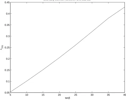
In Fig. 1 we show the variation of the nature of the LSP with tanβ and λ231(MX). Here we have used the two-loop RG evolution equations but in fact the results using one-loop evolution are almost identical. Moreover it is easy to check that (at least at one one-loop) ifλ231 is the only non-zero RPV coupling atMZ then it will remain so at all scales, so we can use a simplified set of β-functions in which we only retain λ231.

5 10 15 20 25 30 35 40

0.05 0.1 0.15 0.2 0.25 0.3 0.35 0.4 0.45

Boundary between selectron and stau LSP

tanβ λ 231

Fig. 1: The variation of the nature of the LSP (stau LSP below the line, selectron LSP above).

Once our results agree pretty with those of Ref. [1], although our demarcation line is slightly lower, particularly for larger values of tanβ.

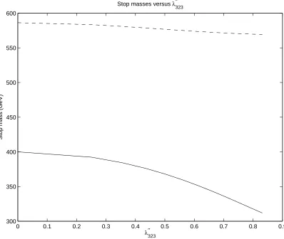
7. The stop masses

The bounds on the λ′′

couplings are much weaker than for the λ and λ′

changes if a particular form is assumed for the quark mixing, such as mixing only in the up-quark or only in the down-quark sector. The bounds are particularly stringent in the down-quark mixing case. Although, as described earlier, we assume the no-mixing case, we expect our results to be qualitatively valid in the general case and therefore we shall display our results up to the perturbativity bound. We consider the dependence of the stop masses on λ′′

323. (In the no-mixing case it is clearly consistent to consider a single non-zero

coupling at all scales.) The mass matrix for up-type quarks has no explicit dependence on the RPV couplings and so the dependence on λ′′₃₂₃ is purely an implicit effect due to the RG evolution. The stop masses are very sensitive to the value of the top mass; here as elsewhere in the paper we take mtop = 174.3GeV. We see that the variation of the stop

masses, especially the light one, on λ′′

323 is considerable.

0 0.1 0.2 0.3 0.4 0.5 0.6 0.7 0.8 0.9

300 350 400 450 500 550 600

Stop masses versus λ′′₃₂₃

λ′′₃₂₃

Stop mass (GeV)

8. Conclusions

We have analysed the effect of including the full set of two-loop β-functions for R-parity violating couplings in a variety of scenarios. Typically we find little difference between the effect of using the full β-functions and that of using the one-loop β-functions plus two-loop RPC corrections for RPC parameters; though as we see in Table 1 there is quite a substantial difference between the bounds on RPV couplings obtained using the full two-loop β-functions and those obtained using the full one-loopβ-functions–and of course it is desirable from the point of view of consistency to use the full set ofβ-functions. In any event, we hope that future analysts will find the availability of the full set of β-functions for the most general R-parity violating version of the MSSM to be a useful resource[9].

Acknowledgements

References

[1] B.C. Allanach, A. Dedes and H.K. Dreiner, Phys. Rev. D69 (2004) 115002 [2] B. de Carlos and P.L. White, Phys. Rev. D54 (1996) 3427; ibid 55 (1997) 4222 [3] L.J. Hall and L. Randall, Phys. Rev. Lett. 65 (1990) 2939

[4] F. Borzumati, G.R. Farrar, N. Polonsky and S. Thomas, Nucl. Phys. B555 (1999) 53 [5] I. Jack and D.R.T. Jones, Phys. Lett. B457 (1999) 101

[6] J.P.J. Hetherington, JHEP 0110 (2001) 024

[7] I. Jack, D.R.T. Jones and A.F. Kord, Phys. Lett. B588 (2004) 127 [8] D.A. Demir, G.L. Kane and T.T. Wang, Phys. Rev. D72 (2005) 015012 [9] http://www.liv.ac.uk/∼dij/rpvbetas/

[10] I. Jack and D.R.T. Jones Phys. Lett. B415 (1997) 383

[11] I. Jack, D.R.T. Jones and A. Pickering, Phys. Lett. B432 (1997) 114

[12] L.V. Avdeev, D.I. Kazakov and I.N. Kondrashuk, Nucl. Phys. B510 (1998) 289 [13] I. Jack, D.R.T Jones, S.P. Martin, M.T. Vaughn and Y. Yamada, Phys. Rev. D 50,

5481 (1994)

[14] D.R.T. Jones, Phys. Lett. B123 (1983) 45 ; V. Novikov et al, Nucl. Phys. B229 (1983) 381 ; V. Novikov et al, Phys. Lett. B166 (1986) 329 ;

M. Shifman and A. Vainstein, Nucl. Phys. B277 (1986) 456

[15] I. Jack, D.R.T. Jones and A. Pickering, Phys. Lett. B432 (1998) 114 [16] I. Jack, D.R.T Jones and A.F. Kord, Phys. Lett. B579 (2004) 180;

Ann. Phys. 316 (2005) 213

[17] http://www.liv.ac.uk/∼dij/betas

[18] I. Jack and D.R.T. Jones, Phys. Lett. B473 (2000) 102;

I. Jack, D.R.T. Jones and S. Parsons, Phys. Rev. D62 (2000) 125022; I. Jack and D.R.T. Jones, Phys. Rev. D63 (2001) 075010

[19] D.M. Pierce, J.A. Bagger, K.T. Matchev and R.J. Zhang, Nucl. Phys. B491 (1997) 3 [20] E.J. Chun and S.K. Kang, Phys. Rev. D61 (2000) 075012

[21] M. Colless et al, astro-ph/0306581

[22] D. Spergel et al, Astrophys. J. Suppl. 148 (2003) 175