This is a repository copy of Identification of N-state spatio-temporal dynamical systems
using a polynomial model.
White Rose Research Online URL for this paper:
http://eprints.whiterose.ac.uk/74617/
Monograph:
Guo, Y., Billings, S.A. and Coca, D. (2007) Identification of N-state spatio-temporal
dynamical systems using a polynomial model. Research Report. ACSE Research Report
no. 960 . Automatic Control and Systems Engineering, University of Sheffield
[email protected] https://eprints.whiterose.ac.uk/ Reuse
Unless indicated otherwise, fulltext items are protected by copyright with all rights reserved. The copyright exception in section 29 of the Copyright, Designs and Patents Act 1988 allows the making of a single copy solely for the purpose of non-commercial research or private study within the limits of fair dealing. The publisher or other rights-holder may allow further reproduction and re-use of this version - refer to the White Rose Research Online record for this item. Where records identify the publisher as the copyright holder, users can verify any specific terms of use on the publisher’s website.
Takedown
If you consider content in White Rose Research Online to be in breach of UK law, please notify us by
Identification of
N
-state Spatio-Temporal Dynamical
Systems Using a Polynomial Model
Yuzhu Guo, Steve A. Billings and Daniel Coca
Research Report No. 960
Department of Automatic Control and Systems Engineering The University of Sheffield
Mappin Street, Sheffield, S1 3JD, UK
IDENTIFICATION OF
N
-STATE SPATIO-TEMPORAL
DYNAMICAL SYSTEMS USING A POLYNOMIAL
MODEL
Yuzhu Guo, Steve A. Billings and Daniel Coca
Abstract
A multivariable polynomial model is introduced to describe n-state spatio-temporal systems. Based on this model, a new neighbourhood detection and transition rules determination method is proposed. Simulation results illustrate that the new method performs well even when the patterns are corrupted by static and dynamical noise. Keywords: Identification; spatio-temporal system; polynomial model.
1. Introduction
Spatio-temporal systems are a class of dynamical systems which can be studied by discretizing space and time. So that the cells evolve in discrete time steps according to deterministic rules that depend on a neighbourhood of influence. Because complex behaviours of patterns can be generated from simple mathematical constructs, spatio-temporal systems have been used for simulating various complex systems, such as chemical, biological and ecological systems (Baier et al., 2002, Ermentrout, 1998, Filipe and Gibson, 1998, Rekeczky et al., 1997).
Binary cellular automata, which are one of the simplest classes of spatio-temporal systems, have been extensively studied in recent years. Several cellular automata identification methods were introduced (Adamatzky, 1994, Maeda and Sakama, 2003, Richards et al., 1990). These studies were all based on the simple rule table model and none gave a clear neighbourhood structure or a parsimonious expression of the rule. Hence the detection processes can become complicated especially when the neighbourhood becomes large. The identification of the Boolean rule was studied by Yang and Billings (2000a). Yang and Billings (2000b) divided the identification procedure into two stages: neighbourhood detection and rule determination for the first time. The CA-OLS method and several neighbourhood detection approaches were later proposed (Billings and Yang, 2003, Mei et al., 2005, Zhao and Billings, 2006).
Binary cellular automata however can only be applied to systems with two states o and 1. But there are many processes that exhibit more than two states one famous example is excitable media in which any cell can take on three states: quiescent, excited and refractory. However there are very few studies on the identification of n -state spatio-temporal systems. In this paper a polynomial model of n-state spatio-temporal system is given for the first time, and a completely new approach for the identification of n-state spatio-temporal systems is proposed including neighbourhood detection and rule determination.
is introduced in section 3 and it is proved that this model can be used to describe this class of spatio-temporal systems exactly. A neighbourhood detection approach using the polynomial model is given in section 4. To show the validity of the new methods, an example is provided in section 5 and two kinds of noise are considered. Finally, conclusions are given in section 6.
2. N-state Spatio-Temporal Systems
An n-state spatio-temporal system is specified by a triple <S R f, , > of cell state set S, neighbourhood R and cell-state transition function :f Sd →S, where n denotes the
size of the state set S and d is the size of the neighbourhood R. The states of the n -state spatio-temporal system come from a finite -state set S, which is represented by
{
0,1, 2,L ,n−1}
. All cells change states synchronously at discrete time steps. The next state of each cell depends on the states of the neighbouring cells at a past time according to an update rule. The neighbourhood of a cell is the set of cells in both the spatial and temporal dimensions that are directly involved in the evolution of the cell. The neighbourhood, denoted as R, is a d-tuple(
ξ ξ1, ,1L ,ξd)
. The transition rules are afunction : d
f S →S. The state ( )f R is the state of a cell whose d neighbours were at states R=
(
ξ ξ1, , ,1 L ξd)
at a past time. The function :m
f S →S expresses the deterministic dependence between a cell and its neighbourhood.
The state set of the neighbourhood is the Cartesian product d
S = × × ×S S L S of states of all the neighbours that gives all the state combinations of these neighbours. The function values at setSd, (f Sd), uniquely determine the transition rules of the
spatio-temporal system. Because the domain Sd is finite, the function may be expressed by
simply tabulating all the arguments d
R∈S and their corresponding function valuesc= f R( ). Each pair ( , )c R is named as a case and there are nd cases for an n
-state d-neighbourhood spatio-temporal system.
For a spatio-temporal pattern, the collection of all cell states in the grid at some time step is called a configuration. A sequence of configurations of a spatio-temporal pattern is denoted asC0, , ,L Ct L , in which each configuration includes all cell states.
Here, C0 is the initial configuration of the spatiotemporal system and Ct represents the configuration of the spatiotemporal system at time t (Maeda and Sakama, 2003). This paper focuses on the identification of patterns in which all cells change synchronously in discrete time steps according to local and identical transition rules. In other words, all cells use the same rules, and the rules are applied to all cells at the same time. The underlying lattice is an infinite rectangular grid throughout this paper.
3. Model for an N-state Spatio-Temporal System
3.1 Table form model
Local transition rules express the deterministic dependence between the cell and its neighbourhood. For each case of a neighbourhood, d
local transition rule: by a formula, by a plot, by an algorithm and so on. The most intuitive approach is where the transition table is simply tabulating for all possible cases, that is, all cases of neighbourhood d
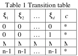
S and the corresponding cell values (f Sd). An example of a table model of an n-state, d-neighbourhood spatio-temporal system with a local transition rule is given as Table 1. Each row represents an evolution case. Columns ξ1 ~ ξd show all state combinations of the neighbourhood, and the values in
[image:5.612.244.373.192.285.2]columns c determine the transition rules.
Table 1 Transition table
1
ξ ξ2 … ξd c
0 0 … 0 * 0 0 … 1 *
M M M M M
n-1 n-1 … n-1 *
3.2 Polynomial form model
The transition table is a basic representation of the local transition rules and it is widely used. However it is tedious especially when the number of cases is very large. In this part a new parsimonious polynomial form model is presented to replace the table form expression.
Yang and Billings (2000b) showed that 2-state spatio-temporal systems, binary cellular automata systems, can be exactly expressed by a polynomial. This conclusion will now be extended to n-state spatio-temporal systems to show that n-state spatio-temporal systems can be exactly expressed by a polynomial. This development will in turn enable the introduction of a new class of neighbourhood detection and rule identification procedures for n-state spatio-temporal systems.
Denote the count of the finite state of cells as n and the size of the neighbourhood as d, let c represent a cell in this spatio-temporal system and R=( , ,ξ ξ1 2 L ξd) represent the
neighbourhood of c . For αi=
(
α αi1, i2,L ,αid)
,αij ≤ −n 1 , constructmonomials 1 2
1 2
i i i id
i d
P =Rα =ξ ξα α L ξα ,i=1, 2,L ,nd and polynomial
1
d
n i i i
P θP
=
=
∑
, wherei
θ are the parameters of this polynomial. It will be shown that an n-state, d -neighbourhood spatio-temporal system can be exactly represented by the polynomial model
1
d
n i i i
P θP
=
=
∑
. Such a polynomial will be constructed in this section.a multivariate polynomial model at the case set d
S . In other words, there is a polynomial which has the same values at all cases listed in the table. Hence, the aim is to find a polynomial which goes exactly through these points. To find a polynomial equivalent to the transition table at set Sd is a problem of multivariate polynomial
interpolation. A multivariate interpolation polynomial in Lagrange form will be constructed as follows.
To illustrate the simple idea behind normal form interpolation, univariate Lagrange interpolation will be briefly considered. Polynomial interpolation is the interpolation of a given data set by a polynomial. In other words, given some data points, the aim is to find a polynomial which goes exactly through these points. A Lagrange polynomial is a linear combination of Lagrange fundamental polynomials. Given a set of data points ( ,x y0 0),L , ( ,x yk k) , the Lagrange polynomial is
0
( ) ( )
k j j j
L x y l x
=
=
∑
, here0,
( ) k i
j
i i j j i
x x l x x x = ≠ − = −
∏
are the Lagrange fundamental polynomials. As can easily be seen, ( )i
l x is a polynomial and has degree k and ( )l xi j =δij. Thus function ( )L x is a polynomial with degree k and
0
( ) ( )
k
i j j i
j
L x y l x y
=
=
∑
= .The univariate Lagrange polynomial interpolation can be easily extended to a multivariate polynomial by the tensor product of univariate interpolation polynomials. It was noted above that the state set of the neighbourhood is the Cartesian product
d
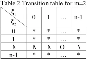
[image:6.612.232.382.483.584.2]S = × × ×S S L S of states of the neighbours. For every neighbour, the state can be any one of the states ranging from 0 to n-1. Rearranging the transition table in the d+1 dimensional space, every dimension of ξ1 ~ ξd has n points. For example, when d=2, Table 1 can be rearranged as shown in Table 2.
Table 2 Transition table for m=2
1
ξ
2
ξ 0 1 … n-1
0 * * … *
1 * * … *
M M M O M
n-1 * * … *
For each dimensionξi , a 1 dimensional Lagrange fundamental polynomial set
{
1( ), ( )2 ( )}
i i i i i in i
L = l ξ l ξ L l ξ can be constructed as
1 0, 1 ( ) ( ) n i ij
k k j
k l j k ξ − = ≠ − − = −
∏
, that is, lij =1 ifξ =i j and lij =0 elsewhere.Denote the indexes ( , ,1 2 , ) d
d S
γ = γ γ L γ ∈ . Computing the tensor product of these
is
{
}
1 21, 2, ,
|
d
d
L= h hγ =l γl γ L l γ , yields the multivariate Lagrange fundamental polynomials, which give a 1-1 mapping with the cases in the transition table.
1 2
1 2
1 : ( , , , ) 0 : ( , , , )
d d if h if γ
ξ ξ ξ γ
ξ ξ ξ γ
=
= ≠
L
L (1)
Define the interpolation polynomial as
(
1, ,2)
( )(
1, ,2)
dd d
S
g f hγ
γ
ξ ξ ξ γ ξ ξ ξ
∈
=
∑
L L .
Obviously, g R
( )
=c holds for ( , )∀ R c in the transition table. Equally, g(
ξ ξ1, ,2 L ξd)
can be expressed as 1 2
1 1 1 d d n i d i α α α
θ ξ ξ ξ
=
∑
L , where θi are parameters of the polynomialand 0≤αi≤ −n 1 . Then the n-state d-neighbourhood spatio-temporal system is described by the polynomial modelg
(
ξ ξ1, ,2 L ξd)
exactly. Define a monomial termset
{
1 2}
1 2
d
d
T = ξ ξα α L ξα , where 0≤αi ≤ −n 1. Arrange all the terms in set T in an increasing order, that is, the terms of lower degree come before the terms of higher degree, into a monomial term vector d 1 1 2 d , i
n n
P × =p p L p p ∈T . Hence the polynomial model can now be described in compact form asc= ΘP , where d 1
n
P × is the monomial term vector and 1 d 1 2 d
T
n θ θ θn
×
Θ = L is the parameter vector.
Based on the results above, the polynomial model as a representation of n-state, d -neighbourhood spatio-temporal systems has the following advantages:
1) Provides an accurate description of n-state spatio-temporal systems; 2) the model is linear-in-the-parameter and these parameters can be estimated using least squares based estimation methods; 3) the number of terms in the polynomial is d
n which only depends on the number of states (n) and the size of neighbourhood (d), but does not rely to the lattice structure or the dimension of the spatio-temporal system.
4. Neighbourhood Detection
Neighbourhood detection is a core problem in the identification of spatio-temporal systems because once the neighbourhood and the model terms are known it is really easy to identify the model. In this section, a new neighbourhood detection method based on the new polynomial model is introduced.
4.1 Candidate transition table
Assume that a candidate neighbourhood denoted asW =
{
ξ ξ1, ,2 L ξd,L ξd d+ 1}
, whichis large enough to cover the potential neighbourhood denoted asR, is given. Without loss of generality, let R=
{
ξ ξ1, ,2 L ,ξd}
be the true neighbourhood of the d -neighbourhood spatio-temporal system. That is, W is a proper superset of R and{
ξd+1,ξd+2,L ,ξd d+ 1}
= −W R is the relative complement of R inW. For an n-statespatio-temporal system whose state set of all cells isS, the state set of the candidate neighbourhood is Sd d+ 1 . Define a function 1
: d d
1 2 1 1 2
( , , d, d d ) ( , , d)
vξ ξ L ξ L ξ + = f ξ ξ L ξ . Hence, function v with d+d1 neighbours as inputs can describe the d-neighbourhood system as the transition function f does. Obviously, the values of function v do not rely on the states of neighboursξd+1,L ,ξd d+ 1. That is the value of function v does not change with the
difference of the states of combination of (ξd+1,ξd+2, ,L ξd d+ 1) if the states of
1 2
( , ,ξ ξ L , )ξd are fixed. Tabulate all the cases ( , ,ξ ξ1 2 L , ,ξd L ,ξd d+ 1, )c to give another transition table, namely the candidate transition table, which is different from the transition table consisted of( , , , , )ξ ξ1 2 L ξd c .
Spatio-temporal systems are autonomous systems and there are no external inputs which influence the evolution. An identification procedure can therefore only be established based on the data from the observed spatio-temporal patterns. Hence, the transition table has to be obtained by extracting all cases from a spatio-temporal pattern one by one, which can be extremely tedious. In addition, because of the unknown exact neighbourhood, an initial candidate neighbourhood should be used, which makes the condition worse. Fortunately, a terse polynomial model was proposed in section 3. This model is equivalent to the candidate transition table and can describe the pattern exactly. Construct all the monomial terms
1 1 2
1 2 1 , 0 1
d d
d d i n
α α α
ξ ξ ξ + α
+ ≤ ≤ −
L arranging all the terms in an increasing order as a term
vector, namely, 1 1 1 1 1
1 2 1 2 1
1 n n n
d d
P= ξ ξ L ξ ξ− − L ξ +− . Hence the polynomial model vcan be expressed as
1
1
2
1 1 1 1 1
1 2 1 1 2 1 2 1
( , , ) 1
d d
n n n
d d d d
n
v
θ θ
ξ ξ ξ ξ ξ ξ ξ ξ
θ + − − − + + =
L L L
M (2)
Once data has been collected from the patterns the parameters 1 2 d d1
T n
θ θ θ +
L
can be estimated using a least squares based method.
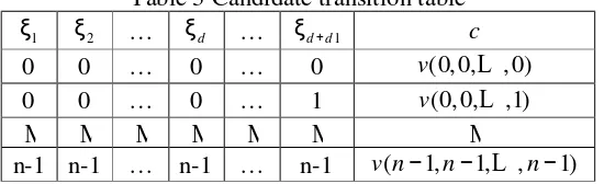
Then based on the polynomial model above, construct a candidate transition table as in Table 3, which describes the pattern exactly, where the columns ξ1 ~ ξd d+ 1 give all
[image:8.612.171.446.599.683.2]the state combinations of the neighbourhood and column c gives the corresponding values of functionv.
Table 3 Candidate transition table
1
ξ ξ2 … ξd … ξd d+ 1 c
0 0 … 0 … 0 v(0, 0,L , 0) 0 0 … 0 … 1 v(0, 0,L ,1)
M M M M M M M
n-1 n-1 … n-1 … n-1 v n( −1,n−1,L ,n−1)
Denote a cell in a spatio-temporal pattern asc, and the associated neighbourhood as R and a candidate neighbourhood asW , where W ⊃R . Let E=W −R , which consists of cells that are in the candidate neighbourhood but not in the true neighbourhood. Denote the state set of this spatio-temporal pattern as S =
{
0,1,L ,n−1}
. Define the operator ⊕ as the modulo n addition operator. Define a function ( )f x , whose domain is the cell state setS, as cyclic symmetric about variable x if f x( )= f x( ⊕1) for ∀ ∈x S , in other words,(0) (1) ( 1)
f = f = =L f n+ . From the above discussion, the evolution of cell c does not depend on the cells in setE, that is, function v( , ,ξ ξ1 2 L ξd,L ξd d+ 1) is cyclic
symmetric about the cells in set E . Contrarily, function v( , ,ξ ξ1 2 L ξd,L ξd d+ 1) is cyclic asymmetric about cells in neighbourhoodR. This property can be used to eliminate the cells of E from the candidate neighbourhood W to determinate the exact neighbourhood R . For convenience, a normalised cyclic asymmetric loss function n( )
ca i
J ξ is introduced to evaluate the cyclic asymmetry with respect toξi. This loss function can be defined as
(
)
(
( ) ( ) ( ) ( ) ( ) ( ))
1 1 1 1
( ) ( , , , , ) ( , , 1, , )
n k k k k k k
ca i i d d i d d
k
J ξ =
∑
sign w v ξ L ξ L ξ + −vξ L ξ ⊕ L ξ + (3)where k is the index of the data from the pattern and the function ( )w x is defined as w x( ) 1= if | |x ≤ε and w x( ) 0= , otherwise. This means that for the data
( ) ( ) ( ) ( )
1 1
( k , , k , , k , k )
i d d c
ξ L ξ L ξ + from the spatio-temporal pattern, the loss function of ξi increases by 1, if the function ( ) ( ) ( )
1 1
( k , , k , , k )
i d d
vξ L ξ L ξ + is cyclic asymmetry aboutξi,
otherwise, the value of the loss function will not change. Hence, if the initial values of the loss function about ξ ξ1~ d d+ 1 are set to zeros, those loss functions about the cells
in set E will still be zero after all the data has been considered. For a noisy pattern a threshold Jcutoff should be selected. The neighbourξj in the candidate neighbourhood should be eliminated if n( )
ca j cutoff
J ξ < J . In practice the state set Sd d+ 1 and values 1
( d d )
v S + are used as the data set to evaluate the loss function in order to reduce the computational expense.
In practice, another problem must be considered. For a spatio-temporal system with n states and d+d1 candidate neighbours, the number of cases should bend d+ 1. This number will be enormous when n and d+d1 are very large. Because the data available will always be finite, the pattern may not include all these cases and this destroys the cyclic symmetry of the function. Hence a mask function is introduced to deal with the problem by differentiating the cases that are not included in the pattern and those that are included. The mask function can be constructed as follows. From the conclusion in section 3, nd d+ 1 Lagrange fundamental polynomials can be
fundamental polynomials can be used as the mask function. Considering the values of a Lagrange fundamental polynomial based on all the data from a pattern, if the values are zero for all the conditions, the corresponding case is not included in this pattern.
4.3 Identification of n-state spatio-temporal patterns
The procedure for the identification of n-state spatio-temporal patterns can now be summarised as:
(1) Select a candidate neighbourhoodW, which is larger enough to cover the potential neighbourhood.
(2) Construct the polynomial terms d 1 1 2 d
n n
P × = p p L p and give the structure of the polynomial modelv( , , ,ξ ξ1 2 L ξd d+ 1)= ΘP .
(3) Collect data from the spatio-temporal pattern and estimate the parameters Θ in the polynomial model.
(4) Eliminate the cases not included in the pattern from the candidate transition table using the mask function.
(5) Select the threshold value as 1
1
1
( ) 2( 1)
d d n
cutoff ca j
j
J J
d d ξ
+ =
=
+
∑
and calculate the lossfunction of cyclic asymmetric n( )
ca i
J ξ about all the ξi’s based on the candidate pseudo transition table. Eliminate the neighbour ξi from the candidate neighbourhood, ifJca( )si <Jcutoff.
(6) Repeat step (5) until the correct neighbourhood is obtained.
(7) Using the correct neighbourhood from step (5), repeat step (2) and (3), to get the final polynomial model of the spatio-temporal pattern.
After obtaining the polynomial model, two kinds of prediction methods can then be used to predict the behaviours of the spatio-temporal system: one step ahead prediction and model predicted output or many steps ahead prediction. Model predicted output is a more strict criteria for evaluation the performance of the estimator than the one step ahead prediction and is used to validate the identified model in this paper.
5. Simulation Analysis
For simplicity, in this section only one example of a 3-state, 3-neighourhood 1- dimensional spatio-temporal noise free pattern and two kinds of noisy patterns will be considered. But lots of simulations have been done to illustrate the validity of these new methods, including examples with more states and more neighbours, including examples of 2-dimensional patterns.
5.1 Effects of noise
There are two kinds of noise in spatio-temporal systems due to different origins: static noise and dynamical noise. Static noise, introduced by external factors, does not involve the evolution of the spatio-temporal pattern. It can be added after the evolution has finished. Unlike static noise, dynamical noise is introduced by internal factors and involves the evolution of the spatio-temporal pattern. Dynamical noise is added into the patterns as part of the evolution of the patterns and is a complex effect.
original pattern
0 1 2
pattern with 5% static noise
0 1 2
pattern with 5% dynamic noise
0 1 2
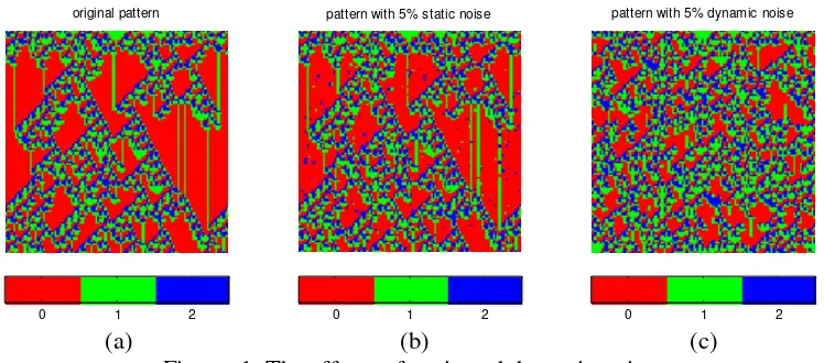
[image:11.612.120.494.166.331.2](a) (b) (c) Figure. 1. The effects of static and dynamic noise.
(a) noise free pattern (b) pattern with 5% static noise (c) pattern with 5% dynamic noise
Figure 1 shows the effect of static noise and dynamic noise on a spatio-temporal pattern. The pattern disturbed by 5% dynamic noise in Figure 1 (c) looks significantly different from the original pattern Figure 1 (a) than the pattern disturbed by 5% static noise in Figure 1 (b). However simulation results shows that, compared with dynamical noise, static noise is more challenging for the identification of spatio-temporal patterns since the cells corrupted by dynamic noise continue to comply with the transition rules, while the patterns corrupted with static noise do not.
5.2 Simulation examples
Three examples are presented in this section. The first example, the identification of a 1-D, 3-state, 3-neighbourhood pattern, is described in more detail to show all the steps in the identification. For the other two examples, only the identification results are given for simplicity.
5.2.1 Identification of a 1-dimensional, 3-state, 3-neighbourhood pattern
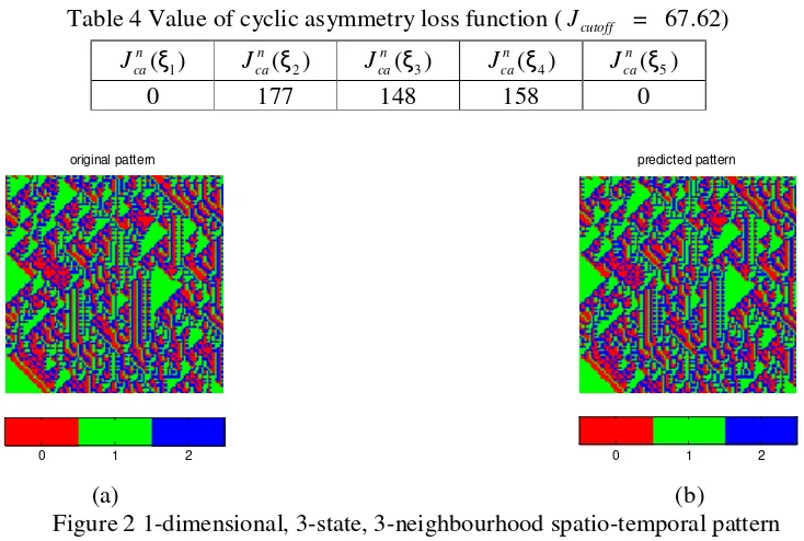
A 1-dimentional, 3-state, 3-neighbourhood pattern with a von Neumann neighbourhood structure on a 100×100 lattice is shown in Figure 2 (a). Half the pattern in Figure 2 (a) was taken as the data set used for model identification. Denote a cell in this 1 dimensional pattern at position j and time step t as t
j
c . Select a candidate neighbourhood
{
1 1 1 1 1}
2 1 1 2
t t t t t
j j j j j
W = c−− c−− c− c−+ c−+ denoted as
{
ξ ξ ξ ξ ξ1, , , ,2 3 4 5}
. Construct the 1 3× 5 termvector 2 2 2 2 2
1 2 1 2 3 4 5
1
function v
(
ξ ξ ξ ξ ξ1, , , ,2 3 4 5)
as a linear combination of these terms that isv(
ξ ξ ξ ξ ξ = Θ1, , , ,2 3 4 5)
P . Collect data from the pattern and estimate the parameter vectorΘ. For simplicity, the results are not given here. The candidate transition table can then be constructed using the functionv. There are 53 cases in this table. All these cases are then checked with the mask function. Seven cases of 243 are not included in this pattern and were eliminated from the candidate transition table. Calculating the cyclic asymmetry loss function about each cell in the candidate neighbourhood, gave the results in Table 4. Selecting half of the average value of all the n( )
ca j
J ξ ’s as the threshold value, that is
5 1 1 ( ) 2 5 n
cutoff ca j
j
J J ξ
=
=
×
∑
=67.62. ξ1 and ξ5were eliminated from the candidate neighbourhood because n( ),1 n( )5
ca ca
J ξ J ξ were less thanJcutoff. The detected neighbourhood R is
{
ξ ξ ξ2, ,3 4}
, that is, the left shifted von Neumann structure. The polynomial model can then be built using the detected neighbourhood as(
2, ,3 4)
f ξ ξ ξ =ξ2 - ξ ξ2 3 +0.5 2
2 3
ξ ξ + 2 2 3
ξ ξ -0.5 2 2
2 3
ξ ξ -ξ4+7ξ ξ2 4-4 2
2 4
ξ ξ +7.5ξ ξ3 4
-21.375ξ ξ ξ2 3 4+9.375 2
2 3 4
ξ ξ ξ -3 2
3 4
ξ ξ +8.875 2
2 3 4
ξ ξ ξ -3.875 2 2
2 3 4
ξ ξ ξ
+ 2 4
ξ -4 2 2 4
ξ ξ +2 2 2
2 4
ξ ξ -4 2 3 4
ξ ξ +12.375 2 2 3 4
ξ ξ ξ -5.375 2 2
2 3 4
ξ ξ ξ +1.5 2 2
3 4
ξ ξ
-5.375 2 2
2 3 4
ξ ξ ξ +2.375 2 2 2
2 3 4
ξ ξ ξ (4)
[image:12.612.125.492.432.679.2]Using the initial condition of the pattern in Figure 2 (a) as the initial condition with the polynomial model as the rule, the model predicted output pattern is shown in Figure 2 (b).
Table 4 Value of cyclic asymmetry loss function (Jcutoff = 67.62)
1
( )
n ca
J ξ Jcan( )ξ2 Jcan( )ξ3 Jcan( )ξ4 Jcan( )ξ5
0 177 148 158 0
original pattern
0 1 2
noised pattern (dynamic 0%)
0 1 2
predicted pattern
0 1 2
(a) (b)
Figure 2 1-dimensional, 3-state, 3-neighbourhood spatio-temporal pattern (a) the data set used in the identification; (b) the predicted pattern using the
5.2.2 Identification of noisy patterns
In Figure 3 (a), a 1-dimensional, 3-state, 3-neighbourhood spatio-temporal is shown. Then 5% static noise was added to the pattern in Figure 3 (a) and the noisy pattern is shown in figure 3 (b). Half the pattern in figure 3 (b) was used as the data set for model identification. The values of loss functions about every cell in the candidate neighbourhood are given in Table 5. It is shown in Table 5 that cells ξ1 and ξ5 should
be eliminated from the candidate neighbourhood to give the true neighbourhood with a von Neumann structure. The model predicted output pattern based on the identified model is shown in figure 3 (c).
original pattern
0 1 2
noised pattern (static 5%)
0 1 2
predicted pattern
0 1 2
[image:13.612.121.498.210.373.2](a) (b) (c)
[image:13.612.127.502.551.725.2]Figure 3 1-dimentional, 3-state, 3-neighbourhood spatio-temporal pattern (a) the original pattern; (b) 5% static noisy pattern; (c) the predicted pattern
Table 5 Value of cyclic asymmetry loss function (Jcutoff = 68.88)
1
( )
n ca
J ξ n( )2
ca
J ξ n( )3
ca
J ξ n( )4
ca
J ξ n( )5
ca
J ξ
22 152 147 147 24
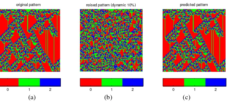
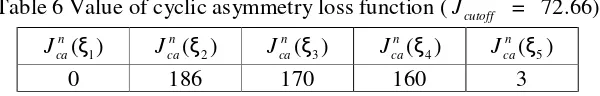
The same pattern as in Figure 3 (a) is given in Figure 4 (a), but now the pattern was corrupted by 10% dynamic noise to give the pattern in Figure 4 (b). This noisy pattern was then used as the data set to identify the model. Table 6 shows that this pattern was a von Neumann structure. The model predicted output pattern based on the identified model is given as Figure 4 (c).
original pattern
0 1 2
noised pattern (dynamic 10%)
0 1 2
predicted pattern
0 1 2
Figure 4 1-dimensional, 3-state (0-red, 1-green, 2-blue), 3-neighbourhood pattern (a) the original pattern; (b) the 10% dynamical noisy pattern; (c) the predicted pattern
Table 6 Value of cyclic asymmetry loss function (Jcutoff = 72.66)
1
( )
n ca
J ξ n( )2
ca
J ξ n( )3
ca
J ξ n( )4
ca
J ξ n( )5
ca
J ξ
0 186 170 160 3
6. Conclusions
A complete solution to the identification of n-state spatio-temporal systems has been introduced in this paper including algorithms for neighbourhood detection and the determination of the transition rules. The linear-in-the-parameters polynomial model provides a simple and accurate representation of n-state spatio-temporal systems. The simulation results show that the neighbourhood detection method is effective and is not sensitive to less than 10% dynamic noise (evolutionary noise), and 5% static noise (measurement noise). However this does not mean the polynomial model extracted based on the correct neighbourhood is accurate enough to exactly predict the pattern, because some transition rules may be more sensitive to noise than others and an exact estimation may only be extracted at lower noise levels. It has also been shown that the neighbourhood detection method in this paper is effective for spatio-temporal patterns which are incomplete.
Acknowledgment
The authors gratefully acknowledge support from the UK Engineering and Physical Sciences Research Council (EPSRC).
References
ADAMATZKY, A. I. (1994) Identification of Cellular automata, New York, Taylor & Francis.
BAIER, G., MÜLLER, M. & ØRSNES, H. (2002) Excitable spatio-temporal chaos in a model of glycolysis. Journal of Physical Chemistry B, 106, 3275-3282. BILLINGS, S. A. & YANG, Y. (2003) Identification of the neighborhood and CA
rules from spatio-temporal CA patterns. IEEE Transactions on Systems, Man, and Cybernetics, Part B: Cybernetics, 33, 332-339.
ERMENTROUT, B. (1998) Neural networks as spatio-temporal pattern-forming systems. Reports on Progress in Physics, 61, 353-430.
FILIPE, J. A. N. & GIBSON, G. J. (1998) Studying and approximating spatio-temporal models for epidemic spread and control. Philosophical Transactions of the Royal Society of London Series B Biological Sciences, 353, 2153-2162.
MAEDA, K. I. & SAKAMA, C. (2003) Discovery of Cellular Automata Rules Using Cases. LECTURE NOTES IN COMPUTER SCIENCE, 360-368.
REKECZKY, C., TAHY, A., VEGH, Z. & ROSKA, T. (1997) CNN-based spatio-temporal nonlinear filtering and endocardial boundary detection in echocardiography. International Journal of Circuit Theory and Applications, 27, 171-207.
RICHARDS, F. C., MEYER, T. P. & PACKARD, N. H. (1990) Extracting cellular automaton rules directly from experimental data. Physica D: Nonlinear Phenomena, 45, 189-202.
YANG, Y. & BILLINGS, S. A. (2000a) Extracting Boolean rules from CA patterns. IEEE Transactions on Systems, Man, and Cybernetics, Part B: Cybernetics, 30, 573-581.
YANG, Y. & BILLINGS, S. A. (2000b) Neighborhood detection and rule selection from cellular automata patterns. IEEE Transactions on Systems, Man, and Cybernetics Part A:Systems and Humans., 30, 840-847.