The wavelet-NARMAX representation : a hybrid model structure combining polynomial models with multiresolution wavelet decompositions

This is a repository copy of

The wavelet-NARMAX representation : a hybrid model

structure combining polynomial models with multiresolution wavelet decompositions

.

White Rose Research Online URL for this paper:

http://eprints.whiterose.ac.uk/1972/

Article:

Billings, S.A. and Wei, H.L. (2005) The wavelet-NARMAX representation : a hybrid model

structure combining polynomial models with multiresolution wavelet decompositions.

International Journal of Systems Science, 36 (3). pp. 137-152. ISSN 1464-5319

https://doi.org/10.1080/00207720512331338120

[email protected] https://eprints.whiterose.ac.uk/

Reuse

Unless indicated otherwise, fulltext items are protected by copyright with all rights reserved. The copyright exception in section 29 of the Copyright, Designs and Patents Act 1988 allows the making of a single copy solely for the purpose of non-commercial research or private study within the limits of fair dealing. The publisher or other rights-holder may allow further reproduction and re-use of this version - refer to the White Rose Research Online record for this item. Where records identify the publisher as the copyright holder, users can verify any specific terms of use on the publisher’s website.

Takedown

If you consider content in White Rose Research Online to be in breach of UK law, please notify us by

White Rose Research Online

http://eprints.whiterose.ac.uk/

This is an author produced version of a paper published in International Journal

of Systems Science.

White Rose Research Online URL for this paper:

http://eprints.whiterose.ac.uk/1972/

Published paper

Billings, S.A. and Wei, H.L. (2005) The wavelet-NARMAX representation : a

hybrid model structure combining polynomial models with multiresolution wavelet

decompositions. International Journal of Systems Science, 36 (3). pp. 137-152.

Prepublication draft of the paper published in

International Journal of Systems Science, Vol. 36, No. 3, 20 February 2005, 137–152

The Wavelet-NARMAX Representation: A Hybrid Model Structure Combining

Polynomial Models with Multiresolution Wavelet Decompositions

S.A. Billings and H.L. Wei

Department of Automatic Control and Systems Engineering, University of Sheffield Mappin Street, Sheffield, S1 3JD, UK

[email protected] , [email protected]

Abstract: A new hybrid model structure combing polynomial models with multiresolution wavelet decompositions is

introduced for nonlinear system identification. Polynomial models play an important role in approximation theory,

and have been extensively used in linear and nonlinear system identification. Wavelet decompositions, in which the

basis functions have the property of localization in both time and frequency, outperform many other approximation

schemes and offer a flexible solution for approximating arbitrary functions. Although wavelet representations can

approximate even severe nonlinearities in a given signal very well, the advantage of these representations can be lost

when wavelets are used to capture linear or low-order nonlinear behaviour in a signal. In order to sufficiently utilise

the global property of polynomials and the local property of wavelet representations simultaneously, in this study

polynomial models and wavelet decompositions are combined together in a parallel structure to represent nonlinear

input-output systems. As a special form of the NARMAX model, this hybrid model structure will be referred to as the

WAvelet-NARMAX model, or simply WANARMAX. Generally, such a WANARMAX representation for an

input-output system might involve a large number of basis functions and therefore a great number of model terms.

Experience reveals that only a small number of these model terms are significant to the system output. A new fast

orthogonal least squares algorithm, called the matching pursuit orthogonal least squares (MPOLS) algorithm, is also

introduced in this study to determine which terms should be included in the final model.

Keywords: Nonlinear system identification; NARMAX models; wavelets; orthogonal least squares.

1. Introduction

Modelling and identification of nonlinear systems have been extensively studied in recent years, and several

model structures and modelling approaches have been developed. These include the polynomial NARMAX

(Nonlinear AutoRegressive Moving Average with eXogenous inputs) model (Billings and Leontaritis 1982,

Leontaritis and Billings 1985), neural networks (Chen et al. 1990b, Chen and Billings 1992, Billings and Chen

1998, Yamada and Yabuta 1993, Delgado et al. 1995), radial basis function networks (Chen et al 1990a, 1992),

wavelet networks (Zhang and Benveniste 1992, Zhang 1997) , fuzzy logic based models (Wang 1992),

neuro-fuzzy networks (Brown and Harris 1994), wavelet multiresolution decompositions (Billings and Coca 1999,

Coca and Billings 2001), support vector machines and kernel methods(Campbell 2002, Lee and Billings 2002),

and other basis function expansion based models. In input-output observational data based modelling, the main

task is to determine a suitable model structure, which involves the smallest number of input variables (the lagged

inputs and outputs for dynamical systems) and adjustable parameters. In practice, however, model parsimony

accuracy and validity have to be considered. Another property often considered while modelling a dynamical

system is the prediction (forecasting) capability of the model.

Among existing model structures, polynomial based model structures play a very important role in linear and

nonlinear system modelling and identification. The well-established linear and nonlinear models such as AR(X),

ARMA(X) (Ljung 1987) and bilinear models, which have been widely used in linear and nonlinear system

modelling, all belong to the polynomial model class and can be viewed as special cases of the polynomial

NARMAX model (Billings and Leontaritis 1982, Leontaritis and Billings 1985, Pearson 1995, 1999).

Polynomials are globally smooth functions. It has been proved that any given continuous function on an infinite

interval can be uniformly approximated using a polynomial (Schumaker 1981). Experience shows that even a

simple polynomial model can track the linear trend of a dynamical system very well. However, a polynomial

model of a low degree possesses a poor ability to track severe nonlinear behaviour, such as jumps and

discontinuities.

Local function expansion based model structures including the wavelet decomposition techniques provide a

powerful tool for representing nonlinear signals, even severely nonlinear signals with discontinuities. Among

almost all the basis functions used for the purpose of approximation, few have had such an impact and spurred so

much interest as wavelets. Wavelet decompositions outperform many other approximation schemes and offer a

flexible capability for approximating arbitrary functions. Wavelet basis functions have the property of

localization in both time and frequency. Due to this inherent property, wavelet approximations provide the

foundation for representing arbitrary functions economically, using just a small number of basis functions.

Wavelet algorithms (Coca and Billing 2001) process data at different scales or resolutions, and this makes

wavelet representations more adaptive compared with other basis functions. Although wavelet decompositions

can represent nonlinear signals very well, the advantage of these decompositions might be lost when a signal

displays linear or low-order nonlinear trends.

In order to sufficiently utilise the global property of polynomial models and the local property of wavelet

representations simultaneously, polynomial models and wavelet decompositions will be combined together in a

parallel way to represent a nonlinear input-output system in the present study. As a special form of the

NARMAX model, this hybrid model structure will be referred to as the WANARMAX model.

One of the common problems in nonlinear system modelling is the curse of dimensionality. Theoretically, an

n-dimensional system should be represented using an n-variate function. However, for large n, it is almost

always true that the observational data only forms a sparse distribution in the space

R

n. Consequently, the identification problem, which can be converted into a regression problem in most cases and for most model

structures, is often ill-posed and various methods have been employed to resolve this problem. One way of

representing a continuous function of several variables is to decompose a multivariate function into a

superposition of a number of continuous functions with fewer variables and this is the essence of Hilbert’s 13th

problem, which was resolved by Kolmogorov. Several applicable approaches have been proposed to realize the

idea of representing multivariate functions using a superposition of a number of functions with fewer variables.

The projection pursuit regression algorithm (Friedman 1981), radial basis function networks (Chen et al 1990b,

1992a), and multi-layer perceptron (MPL) architecture (Haykin 1994) are among the representations that have

been studied for multivariate functions. The existing strategies that attempt to approximate general functions in

NARMAX representation introduced by Billings and Leontaritis (1982, 1985), the multivariate adaptive

regression spline (MARS) method introduced by Friedman (1991), and the adaptive spline modelling of

observational data (ASMOD) introduced by Kavli (1993).

Although experience shows that most systems in practice can be expressed as a supposition of a number of

low-dimensional submodels if the system variables are appropriately selected, a large number of potential model

terms might still be involved when expanding each functional component. Practice and experience show that

often many of the model terms are redundant and inclusion of redundant terms can result in a complex model

structure and the model may become oversensitive to the training data and is likely to exhibit poor generalisation

properties. It is therefore important to determine which terms should be included in the model. A new fast

orthogonal least squares algorithm, called the matching pursuit orthogonal least squares (MPOLS) algorithm, is

introduced in the present paper as one solution to the model term selection problem.

This paper is organised as follows. In Section 2, the wavelet transform and wavelet decompositions are briefly

reviewed. In Section 3, the Wavelet-NARMAX model structure, or simply WANARMAX, is introduced. The

model term selection problem is discussed in Section 4, where a new matching pursuit orthogonal least squares

(MPOLS) algorithm is proposed. Section 5 discusses the implementation of the WANARMAX model. In section

6, two examples are provided to illustrate the applicability of the new modelling framework. Conclusions are

given in Section 7.

2. Multiresolution wavelet decompositions

Assume that the wavelet

ϕ

and the corresponding scaling function

φ

constitute an orthogonal wavelet system.

From wavelet theory (Mallat 1989, Chui 1992, Daubechies 1992), any function can be expressed as

the following multiresolution wavelet decomposition

)

(

2

R

L

f

∈

∑∑

∑

≥

+ =

0 0

0 ( ) ( )

)

( _{, , , ,}

j

j k

k j k j k

j k

k

j x x

x

f

α

φ

β

ϕ

(1)

where

φ

_j,k(x)=2j/2

φ

(2jx−k),

ϕ

_j,k(x)=2j/2

ϕ

(2jx−k), _{j ,k}

0

α

and

β

j,k are the wavelet decomposition

coefficients, j,k∈Z(Zis a set consisting of whole integers), is an arbitrary integer representing the coarsest resolution or scaling level. Note that from Eq. (1) and the property of wavelet multiresolution analysis, any

function can be arbitrarily closely approximated with some sufficiently large integer J, that is, for

any

0

j

)

(

2

R

L

f

∈

ε

>0, there exists a sufficiently large integer J, such that

ε

φ

β

<

−

∑

k

k J k

J x

x

f( ) _{, ,} ( ) (2)

Therefore,

≈

∑

(3) k

k J k

J x

x

This means that the multiresolutin wavelet series decomposition (1) can be replaced by wavelet series (3) with

respect to the orthogonal scaling functions , where J is a sufficiently large scale

number.

) 2 ( 2 ) ( /2

, x x k

J J k

J =

φ

−

φ

Using the concept of tensor products, the multiresolution decomposition (1) can be immediately generalised to

the muti-dimensional case, where a multiresolution wavelet decomposition can be defined by taking the tensor

product of the one-dimensional scaling and wavelet functions (Mallat 1989). The one-dimensional wavelet

decomposition (3) can also be extended to d-dimensional (d >1) case by a tensor product approach as below

f₁₂L_d(x₁(t),x₂(t),L,x_d(t))

(4)

) ) ( 2 , , ) ( 2 , ) ( 2 (

1

2

1, , 1 1 2 2

; d d

J

k k

J J

d k k k

J B x t k x t k x t k

d

d − − −

=

∑

L

L

L

α

wherek=[k₁,k₂L,k_d]T ∈Zdis an d-dimensional index, Bd(⋅) is an d-dimensional scaling function and can

be decomposed as the direct product of d one-dimensional functions

∏

=

=

= d

i i d

d

d x B x x x x

B

1 2

1, , , ) ( ) (

)

( L

φ

(5)

where

φ

(⋅)is a scalar scaling function.

3. The WANARMAX model

The WANARMAX model is formed by combining a polynomial model with wavelet decompositions. In this

study, polynomial NARMAX models and semi-orthogonal multiresolution wavelet decompositions will be

considered and combined in a parallel way.

3.1 The NARMAX representations for nonlinear input-output systems

In the past few decades, modelling and identification techniques for nonlinear systems have been extensively

studied with many applications in approximation, prediction and control. Several nonlinear models have been

proposed in the literature including the NARMAX model representation which was initially proposed by Billings

and Leontaritis (Billings and Leontaritis 1982, Leontaritis and Billings 1985). The NARMAX model takes the

form of the following nonlinear difference equation:

y

(

t

)

=

f

(

y

(

t

−

1

),

L

,

y

(

t

−

n

_y

),

u

(

t

−

1

),

L

,

u

(

t

−

n

_u

),

e

(

t

−

1

),

L

,

e

(

t

−

n

_e

))

+

e

(

t

)

(6)

where is an unknown nonlinear mapping, and are the sampled input and output sequences,

and are the maximum input and output lags, respectively. The noise variable with maximum lag

, is unobservable but is assumed to be bounded and uncorrelated with the inputs and the past outputs. The

model (6) relates the inputs and outputs and takes into account the combined effects of measurement noise,

modelling errors and unmeasured disturbances represented by the noise variable .

f

u

(t

)

y

(t

)

u

n

n

_y

e

(t

)

e

n

)

(t

One of the popular representations for the NARMAX model (6) is the polynomial representation which takes

the function

f

(

⋅

)

as a polynomial of degree

l

and gives the form as

∑

∑ ∑

L

= = =

+

+

+

=

n i n i i i i i i n i i

i

x

t

f

x

t

x

t

f

t

y

i 1 1

0

1 2 1

2 1 2 1 1

1

(

(

))

(

(

),

(

))

)

(

θ

)

(

))

(

,

),

(

),

(

(

1 2 1 2 1 1 1

t

e

t

x

t

x

t

x

f

_i n i i i i i i i n i l

+

+

∑

∑

− =

= l l l

L

L

_L (7)

where

m

i i i₁₂L

θ

are parameters,

n

=

n

y

+

n

u

+

n

e and

∏

, =

=

m k i i i i i i i i i

i

x

t

x

t

x

t

x

t

f

k m m m 1

)

(

))

(

,

),

(

),

(

(

2 1 2 1 2

1 L

L

θ

L

1

≤

m

≤

l

,

⎪

⎩

⎪

⎨

⎧

+

+

≤

≤

+

+

−

−

−

+

≤

≤

+

−

−

≤

≤

−

=

e u y u y u y u y y y y k

n

n

n

k

n

n

n

n

k

t

e

n

n

k

n

n

k

t

u

n

k

k

t

y

t

x

1

))

(

(

1

))

(

(

1

)

(

)

(

(8)

The degree of a multivariate polynomial is defined as the highest order among all terms. For example, the degree

of the polynomial

h

(

x

₁

,

x

₂

,

x

₃

)

=

a

₁

x

₁4

+

a

₂

x

₂

x

₃

+

a

₃

x

₁2

x

₂

x

₃2 is

l

=

2+1+2=5, which is determined by the

last term, . Similarly, a NARMAX model with polynomial degree

l

means that the order of each term

in the model is not higher than .

2 3 2 2 1 3x x x

a

l

The NARX model is a special case of the NARMAX model and takes the form

y

(

t

)

=

f

(

y

(

t

−

1

),

L

,

y

(

t

−

n

_y

),

u

(

t

−

1

),

L

,

u

(

t

−

n

_u

))

+

e

(

t

)

(9)

In this case the variable xk(t) defined in (8) reduces to

⎪⎩

⎪

⎨

⎧

+

=

≤

≤

+

+

−

≤

≤

−

=

u y y y y k

n

n

n

k

n

n

k

t

u

n

k

k

t

y

t

x

1

),

(

1

),

(

)

(

(10)

3.2 The wavelet-based ANOVA expansion

Generally, a multivariate nonlinear function can often be decomposed into a superposition of a number of

functional components via the well known functional analysis of variance (ANOVA) expansions (Friedman

1991, Chen 1993) as below

y

(

t

)

=

f

(

x

1

(

t

),

x

2

(

t

),

L

,

x

n

(

t

))

∑

∑

≤ < ≤ =

+

+

=

n j i j i ij n i i

i

x

t

f

x

t

x

t

f

f

1 1

0

(

(

))

(

(

),

(

))

+

∑

+

L

≤ < < ≤i j k n

k j i ijk

x

x

x

f

1

)

,

,

(

∑

≤ < < ≤

+

n i i i i i i i i m m m

x

t

x

t

x

t

f

L L

L

1 2 1 2 1 1

))

(

,

),

(

),

(

(

+

L

+

f

12Ln

(

x

1

(

t

),

x

2

(

t

),

L

,

x

n

(

t

))

+

e

(t

)

(11)

where the first functional component is a constant to indicate the intrinsic varying trend; , , are

univariate, bivariate, etc., functional components. The univariate functional components represent the

independent contribution to the system output that arises from the action of the ith variable alone; the

0

f

f

i

f

ij

,

L

bivariate functional components represent the interacting contribution to the system output from the

input variables and , etc. Let (k=1,2,…,n) be defined as (8) or (10), the ANOVA expansion (11) can

then be viewed as a special form of the NARMAX or NARX models for dynamic input and output systems.

Although the ANOVA decomposition of the NARMAX model (6) involves up to different functional

components, experience shows that a truncated representation containing the components up to the bivariate or

tri-variate functional terms often provides a satisfactory description of for many high dimensional

problems providing that the input variables are properly selected. It is obvious that adopting a truncated ANOVA

expansion containing only low-dimensional function components does not mean such an approach will always

be appropriate. An exhaustive search for all the possible submodel structures of (11) is demanding and can be

prohibitive because of the curse-of-dimensionality. A truncated representation is advantageous and practical if

the higher order terms can be ignored. In practice, the constant term can often be omitted since it can be

combined into other functional components.

)

,

(

i j ij

x

x

f

i

x

x

_j

x

k

(t

)

n

2

)

(t

y

0

f

It will generally be true that, whatever the data set and whatever the modelling approach, the structure of the

final model will be unknown in advance. It is therefore not possible to know up to how many order functional

components in a truncated ANOVA expansion will be sufficient for a given nonlinear system. This is why model

validation methods, which are independent of the model fitting procedure and the model type, are an important

part of the NARMAX modelling methodology (Billings and Chen 1998). If the model is adequate to represent

the system the residuals should be unpredictable from all linear and nonlinear combinations of past inputs and

outputs. This means that the identified model has captured all the predictable information in the data and is

therefore the best that can be achieved by any model. It is therefore perfectly acceptable to fit a model that

includes just up to one, two or three-dimensional functional terms initially. The model validity tests should then

be applied to test if the model that is obtained has captured all the predictable information in the data. If the

model fails the model validity tests higher order terms should be included in the initial search set and the

procedure should be repeated. It is therefore not necessary to prove that it is always possible to proceed based on

just up to certain order submodels. The identification proceeds a stage at a time and uses model validation as the

decision making process. This is the NARMAX methodology (Billings and Chen 1998), which is implemented

here, and which mimics the traditional approach to analytical modelling. In the latter case the most important

model terms are included in the model initially then the less significant terms are added until the model is

considered to be adequate. This is exactly what the OLS algorithm and the ERR does but based on the data. The

most significant model terms are added first, step by step, a term at a time. The ERR cut-off value is used as a

stopping mechanism but the model should never be accepted without applying model validity tests. If these tests

fail go back and either reduce the ERR cut-off, or allow more complex model terms in the initial model library,

or both and continue until the model validity tests are satisfied.

In practice, many types of functions, such as kernel functions, splines, polynomials and other basis functions

can be chosen to express the functional components in model (11). In the present study, however, mutiresolution

wavelet decompositions will be chosen to describe the functional components. For example, the functional

components

f

_p

(

x

_p

(

t

))

(p=1,2,…,n) and

f

_pq

(

x

_p

(

t

),

x

_q

(

t

))

(

1

≤

p

<

q

≤

n

) can be expressed using the

∑∑

∑

≥ + = 1 1

1 ( ()) ( ())

)) ( ( (_,) _, (_,) _, j j k p k j p k j p k j k p k j p

p x t x t x t

f

α

φ

β

ϕ

,

p

=

1

,

2

,

L

,

n

, (12)

=

∑∑

1 2 2 2 1 2 2 1

2 ( ()) ( ())

)) ( ), (

( (_;)(_,1) _{, ,}

k k q k j p k j pq k k j q p

pq x t x t x t x t

f

α

φ

φ

∑∑∑

≥

+

2 1 2

2 1

2

1 , ( ()) , ( ())

) 1 )( ( , ; j

j k k

q k j p k j pq k k

j

φ

x t

ϕ

x t

β

∑∑∑

≥

+

2 1 2

2 1

2

1 , ( ()) , ( ())

) 2 )( ( , ; j

j k k

q k j p k j pq k k

j

ϕ

x t

φ

x t

β

∑∑∑

≥

+

2 1 2

2 1

2

1 , ( ()) , ( ())

) 3 )( ( , ; j

j k k

q k j p k j pq k k

j

ϕ

x t

ϕ

x t

β

,

1

≤

p

<

q

≤

n

. (13)

3.3 The WANARMAX model

The wavelet-NARMAX model, or simply WANARMAX, which incorporates a polynomial NARMAX model

and a multiresolution wavelet decomposition in a parallel way, can be defined as

) ( )) ( ( )) ( ( )) ( ( )) ( ( )

(t f x t f x t f x t f t e t

y = = P + W + E

ξ

+ (14)

where and (k=1,2,…,n) are defined as in (10), is a

polynomial model; is a wavelet decomposition model; and is a polynomial model with

respect to the noise variable and .The submodels ,

and can be combined into the WANARMAX model (14) in various forms and the

following are some examples

T n

t

x

t

x

t

x

t

x

(

)

=

[

1

(

),

2

(

),

L

,

(

)]

x

k

(t

)

f

( t

x

(

))

P

))

(

( t

x

f

W

f

E

(

ξ

(

t

))

)

(t

e

ξ

(

t

)

=

[

e

(

t

−

1

),

e

(

t

−

2

),

L

,

e

(

t

−

n

_e

)]

T

f

P

( t

x

(

))

))

(

( t

x

f

W

f

E

(

ξ

(

t

))

∑∑

∑

= = = + + = n p n p q q p pq n p p p P t x t x b t x a a t x f 1 1

0 ( ) ( ) ( )

)) (

( (15)

∑∑

∑

= = = + = n p n p q q p pq n p p p W t x t x f t x f t x f 1 1 )) ( ), ( ( )) ( ( )) (

( (16)

∑

∑∑

(17) = = = − − + −

= e ne e

p n p q pq n p p E q t e p t e c p t e c t f 1 1 ) ( ) ( ) ( )) ( (ξ

where the functional components (p=1,2,…,n) and ( ) in (16)

can be expressed using the multiresolution wavelet decompositions.

))

(

(

x

t

f

_{p p}

f

_pq

(

x

_p

(

t

),

x

_q

(

t

))

1

≤

p

<

q

≤

n

For a selected wavelet

ϕ

(⋅) and the scaling function

φ

(⋅), once the maximum lags , and are given, and the initial(coarsest) and highest(finest) resolution scales in the multiresolution decomposition are determined,

the WANARMAX model can be rearranged and converted into a linear-in-the-parameters regression model of

the form

y

n

n

u

n

e

(18) ) ( ) ( ) ( ) ( ) ( 3 2 1 1 1 1 t e t p t p t p t y M k E k E k M j W j W j M i P i P

i + + +

=

∑

∑

∑

= = =

θ

θ

θ

where the regressors piP(t),p (t)and ( W

j p (t)

E

k i=1,2,L,M1;j=1,2,L,M2;k =1,2,L,M3) are related to

model fE( t

ξ

( )), respectively.

θ

iP, and ( W

j

θ

E

k

θ

i

=

1

,

2

,

L

,

M

₁

;

j

=

1

,

2

,

L

,

M

₂

;

k=1,2,L,M₃) are parameters

to be estimated.M₁ =(n_y +n_u +1)(n_y +n_u +2)/2,M3 =n_e and depends on not only the wavelet type

used but also the initial and the highest resolution scales.

2

M

A special case for the WANARMAX model (18) is the Wavelet-NARX, or simply WANARX model

) ( ) ( )

( )

(

2 1

1 1

t e t p t

p t

y

M

j

W j W j M

i

P i P

i + +

=

∑

∑

= =

θ

θ

(19)

Although many functions can be chosen as scaling and/or wavelet functions, most of these are not suitable in

system identification applications, especially in the case of multidimensional and multiresolution expansions. An

implementation, which has been tested with very good results, involves B-spline and B-wavelet functions in

multiresolution wavelet decompositions (Billings and Coca 1999, Coca and Billings 2001, Wei and Billings

2002). B-spline wavelets were originally introduced by Chui and Wang (1992) to define a class of

semi-orthogonal wavelets.

For large and , the model (18) might involve a great number of model terms or regressors. Experience

shows that often many of the model terms are redundant and therefore are insignificant to the system output and

can be removed from the model. An efficient algorithm is required to determine which terms should be included

in the model. The significant model term selection problem is discussed in the next section. y

n

n

u

4. Model term selection

The selection of which terms should be included in the WANARMAX model (18) is vital if a parsimonious

representation of the system is to be identified. For a selected basic wavelet and associated scaling function, once

the initial resolution scale level is given, simply increasing the orders and of the dynamic terms and the

highest resolutions in the multiresolution wavelet model will in general result in an excessively over

parameterised complex model. Fortunately, experience has shown that only a small number of subsets of these

model terms are significant and the remainder can be discarded with little deterioration in prediction accuracy.

Several possible ways can be used to determine which terms are significant and should be included in the model,

including the well-known orthogonal least squares (OLS) algorithm. In this section, the forward orthogonal least

squares (OLS) algorithm is briefly summarised and then a new matching pursuit orthogonal least squares

(MPOLS) algorithm is introduced.

y

n

n

u

The WANARMAX model (18) can be expressed as a linear-in-the-parameters equation of the form

) ( ) ( )

( 1

t e t p t

y M

m m

m +

=

∑

=

θ

(20)

where pm(t)= pmP(t) for

m

=

1

,

2

,

L

,

M

1 , p (t) p (t) for W

m

m =

M

1

+

1

≤

m

≤

M

1

+

M

2 , and

for

) ( )

(t p t

p_m = _mE

M

₁

+

M

₂

+

1

≤

m

≤

M

=

M

₁

+

M

₂

+

M

₃.

θ

_m (m=1,2,L,M ) are parameters to be estimated. Define

} , , 2 , 1 ; 1

: { )

( _{p i M k m}

Pm _{i k}

k ≤ ≤ = L

The model term selection procedure is in fact an iterative process which searches through a nested term set in the

sense that

L

L

⊂

⊂

⊂

⊂

(2) ( )

) 1

( m

P

P

P

(22) This makes both the complexity and the accuracy of the representation based on these term sets increase until a

suitable term set is found, that is, there exists an integer

M

₀ (generally

M

₀

<<

M

), such that the model

(23)

) ( ) ( )

(

0

1

t e t p t

y M

k i

ik k +

=

∑

=

θ

provides a satisfactory representation over the range considered for the measured input-output data.

4.1 The forward orthogonal least squares (OLS) algorithm

A fast and efficient model structure determination approach can be implemented using the forward orthogonal

least squares (OLS) algorithm and the error reduction ratio (ERR) criterion, which was originally introduced to

determine which terms should be included in nonlinear models (Billings et al. 1988, 1989, Korenberg et al. 1988,

Chen et al. 1989). This approach has been extensively studied and widely applied in nonlinear system

identification (see, for example, Chen et al. 1991, Wang and Mendel 1992, Zhu and Billings 1996, Zhang 1997,

Hong and Harris 2001). The forward OLS algorithm involves a stepwise orthogonalization of the regressors and

a forward selection of the relevant terms in (20) based on the error reduction ratio (ERR) (Billings et al. 1988,

1989). The procedure can be briefly summarised as follows:

Consider the linear-in-the-parameters model (20), where the regression matrix with

, N is the length of the observational data set. With the assumption that P is full

rank in columns, then P can be orthogonally decomposed as

]

,

,

,

[

p

₁

p

₂

p

_M

P

=

L

T i i

i

i p p p N

p =[ (1), (2),L, ( )]

WA

P= (24) where

A

is an M×M unit upper triangular matrix and

W

is an

N

×

M

matrix with orthogonal columns

in the sense that M

w

w

w

₁

,

₂

,

L

,

WTW=D

=

diag

[

d

₁

,

d

₂

,

L

,d

_M

]

with . Model (20) can then be expressed as

m T m

m

w

w

d

=

Ξ + = Ξ + Θ

= _PA− _{A WG}

Y ( 1)( ) (25)

where are the observations of the system output, is the

parameter vector, is the vector of the noise signal, and is an

auxiliary parameter vector, which can be calculated directly from

Y

and by means of the property of

orthogonality as

T N y y

y

Y =[ (1), (2),L, ( )] T

M]

, , ,

[

θ

1

θ

2 L

θ

= Θ

T N )]

( , ), 2 ( ), 1 (

[

ε

ε

L

ε

=

Ξ T

M g g g

G=[ 1, 2,L, ]

W

i T i

i T

i

w w

w Y

g = ,

i

=

1

,

2

,

L

,

M

(26)

The number M of all the candidate terms in model (20) is often very large. Some of these terms may be

redundant and should be removed to give a parsimonious model with only terms ( ). Detection

of the significant model terms can be achieved using the OLS procedures described below.

0

M M0 <<M

Assume that the residual signal

ε

(t) in the model (20) is uncorrelated with the past outputs of the system, then the output variance can be expressed as

Ξ Ξ + =

∑

=

T M

i

i T i i T

N w w g N Y Y N

1 1

1

1 2

(27)

Note that the output variance consists of two parts, the desired output

∑

M₌

i i

T i iw w g N

1 2 )

/ 1

( which can be

explained by the regressors, and the part which represents the unexplained variance. Thus

is the increment to the explained desired output variance brought by , and the

i

th error

reduction ratio, , introduced by , can be defined as

Ξ ΞT N )

/ 1 (

∑

=

M

i i

T i i w w g N

1 2 )

/ 1

( p_i

i

ERR pi

% 100 ) ( 2

× =

Y Y

w w g ERR

T i T i i

i 100%

) )( (

)

( 2

× =

i T i T

i T

w w Y Y

w Y

, i=1,2,L,M , (28)

This ratio provides a simple but effective means for seeking a subset of significant regressors. The significant

terms can be selected in a forward-regression manner according to the value of step by step. The

significant terms can be selected in a forward-regression manner according to the value of . Several

orthogonalization procedures, such as Gram-Schmidt, modified Gram-Schmidt and Householder transformation

(Chen et al. 1989) can be applied to implement the orthogonal decomposition. The improved version of this

algorithm (Zhu and Billings 1996) provides a significant reduction in the computations and is advantageous

compared to standard Gram-Schmidt algorithm when dealing with high order MIMO systems. Other recent

studies by Hong and Harris (2001) have proposed other improvements to this procedure. i ERR

i

ERR

Remark 1: The forward orthogonal least squares algorithm for model term selection is described and

expounded in a matrix form here for convenience of introducing and explaining the concept of error reduction

ratio (ERR). In practical identification, however, this algorithm is often implemented in a forward stepwise way

(Wei and Billings 2004). The most significant model terms are added first, step by step, a term at a time. The

ERR cut-off value is used as a stopping mechanism but the model should never be accepted without applying

model validity tests.

Remark 2: The candidate terms that are not chosen in the first step are orthogonalized with respect to all

previously selected basis functions. Because of the orthogonality the

j

th term can be selected in the same way as in the first step.

w

j is the

j

th selected orthogonal term and is the corresponding parameter. Any numerical ill conditioning can be avoided by eliminating the candidate basis functions for which are less

than a predetermined threshold

j

g

i T i

w

w

Remark 3: The assumption that the regression matrix P is full rank in columns is unnecessary in the iterative

forward OLS algorithm(Wei and Billings 2004). In fact, if the M columns of the matrix P are linearly dependent,

and assuming that the rank in columns of the matrix P is L (<M) , then the algorithm will stop at the L-th step.

Remark 4: If required, the procedure can be terminated at the -th step ( ) when

, where

0

M M0 ≤L

ρ

< −

∑

= 0 1 1 M i i

ERR

ρ

is a desired error tolerance called the cutoff, which can be learnt during the

regression procedure. The final model is the linear combination of the M0 significant terms selected from the

M candidate terms

{

p

_i

}

M_i=1

)

(

)

(

)

(

0 1

t

e

t

w

g

t

y

M i i i

+

=

∑

= (29)

which is equivalent to

)

(

))

(

(

)

(

0 1

t

e

t

x

p

t

y

M i i i

+

=

∑

= l l

θ

(30)

where the parameters are calculated from the triangular equation

with and

T OLS M ] , , , [ 0 2 1 ) ( l l l

θ

L

θ

θ

=

Θ (OLS) (OLS)

AG =Θ

T M

OLS _{g g g}

G [ , , , ]

0

2 1 )

( _{= L}

⎥ ⎥ ⎥ ⎥ ⎥ ⎥ ⎥ ⎦ ⎤ ⎢ ⎢ ⎢ ⎢ ⎢ ⎢ ⎢ ⎣ ⎡ = − 1 0 0 1 0 1 0 1 0 0 0 0 , 1 2 1 12 L L M O M M L L M M M M a a a a

A (31)

The entries aij(1≤i< j≤M0) are given in the above OLS algorithm.

Remark 5: The key point in the forward OLS-ERR algorithm is focused on detecting the most significant

model terms from a great number of candidates by introducing an orthogonalization procedure and the concept

of error reduction ratio (ERR). The estimation of the model parameters is only a by-product of the model term

selection procedure. It requires that the orthogonalization should be explicit so that the significant model terms

selected by the algorithm are transparent to the model builders. Many other singular value decomposition

methods including the standard SVD, Krylov subspace and Lanczos bidiagonalizaiton methods, which are

proved to be more numerically stable compared with the present OLS algorithm, can be used to solve linear least

squares problems, where the main task is to estimate the unknown parameters for a given linear equation. These

methods, however, cannot provide any information about which model terms are the most significant. In other

words, for a given linear-in-the-parameters form (20), these methods cannot tell which model terms or regressors

make the most significant contributions to the system output y(t). These methods could however provide an aid

for solving the identification problem by combining the methods with the forward OLS-ERR algorithm. For

example, the most significant model terms could then be selected initially using the forward OLS-ERR algorithm,

4.2 Matching pursuit orthogonal least squares (MPOLS) algorithm

Note that in the forward OLS algorithm, at each step all the unselected regressors are made to orthogonalize

with the previously selected regressors, and most of the computational cost is based on these orthogonalization

transforms. An iterated orthogonal projection algorithm, the matching pursuit method, proposed by Mallat and

Zhang (1993) is a simple regressor selection algorithm which is relatively computationally efficient. But the

matching pursuit algorithm is less efficient than OLS, since the number of regressors selected by the matching

pursuit algorithm is almost always larger than that selected by OLS for the same given threshold value of

approximation accuracy. A trade-off between the efficiency and the computational cost is considered here by

combining the advantages of the forward OLS with the matching pursuit algorithm to create a new algorithm

called the matching pursuit orthogonal least squares (MPOLS) algorithm. The algorithm is described below.

For the output vector in (20), find a vector from the candidate regressor

family , so that is the “best” matching regressor to Y, i.e., makes the mean squared

error of the following linear regression

T

N

y

y

y

Y

=

[

(

1

),

(

2

),

L

,

(

)]

1 l

p

}

,

,

,

{

p

₁

p

₂

L

p

_M

1 l

p

1 l

p

)

(

)

(

)

(

t

c

p

t

t

y

=

_{m m}

+

ξ

_m (32) achieve a minimum in the sense that

⎭

⎬

⎫

⎩

⎨

⎧

₋

=

−

=

∑

∑

∑

= = = N t m m m N t N t

t

p

c

t

y

N

t

p

c

t

y

N

t

N

1 2 1 2 1 2

)]

(

)

(

[

1

min

))

(

)

(

(

1

)

(

1

1 1

1 l l

l

ξ

(33)

The “best” matching regressor can be found using orthogonal projection approach by defining 1 l

p

m T m T m T

p

p

Y

Y

p

Y

=

α

cos

(34)

m T m m T m

p

p

p

Y

Y

p

1

=

cos

α

=

(35)

Such that 2 1 2 2 1 2

)

(

_{m m}

N

t

m

t

=

=

Y

−

p

∑

=

ξ

ξ

m T m m T T

p

p

p

Y

Y

Y

2

)

(

−

=

(36)

Thus

⎭

⎬

⎫

⎩

⎨

⎧

≤

≤

=

m

M

p

p

p

Y

m T m m T

m

,

1

)

(

max

arg

2 1

l

(37)

Set

(

)

(

)

, , , , and

1

1

t

p

t

q

=

_l

w

₁

(

t

)

=

q

₁

(

t

)

g

1

(

Y

w

1

)

/(

w

1

w

1

)

T T

=

(

1 1

)

/(

)

2 1

1

g

w

w

Y

Y

ERR

=

T T

)

(

)

(

)

(

_{1 1}

1

t

=

y

t

−

g

w

t

η

.

At the second step, find a vector from the candidate regressor family 2

l

p

{

p

_m

:

1

≤

m

≤

M

,

m

≠

l

₁

}

, so that

is the “best” matching regrssor to 2

l

p

η

₁. Following the approach in (32) and (33),

l

₂ should be chosen as

⎭

⎬

⎫

⎩

⎨

⎧

≠

≤

≤

=

1 2 ₁

2

,

1

,

)

(

max

arg

l

l

m

M

m

Set

(

)

(

)

. Orthogonalize with as below 2

2

t

p

t

q

=

l

q

2

w

1

1 1 1 2 1 2 2

w

w

w

q

w

q

w

_T T

−

=

(39)

And set

g

2

(

Y

w

2

)

/(

w

2

w

2

)

, , and

T T

=

(

2 2

)

/(

)

2 2

2

g

w

w

Y

Y

ERR

=

T T

η

₂

(

t

)

=

η

₁

(

t

)

−

g

₂

w

₂

(

t

)

. Generally, at step k, select

⎭

⎬

⎫

⎩

⎨

⎧

≠

≠

≠

≤

≤

=

− ₋ 1 2 1 2 1

,

,

,

,

1

,

)

(

max

arg

_k m T m m T k m

k

m

M

m

m

m

p

p

p

l

L

l

l

l

η

(40)

Set

q

(

t

)

p

(

t

)

and orthogonalize with as below

k

k

=

l

q

k

w

1

,

w

2

,

L

,

w

k−1

1 1 1 1 2 2 2 2 1 1 1 1 − − − −

−

−

−

−

=

_k k T k k T k T k T T k T k k

w

w

w

q

w

w

w

w

q

w

w

w

w

q

w

q

w

L

(41)

Calculate

(

)

/(

k

)

, , and set

T k k T

k

Y

w

w

w

g

=

ERR

g

2

(

w

w

k

)

/(

Y

T

Y

)

T k k

k

=

η

k

(

t

)

=

η

k−1

(

t

)

−

g

k

w

k

(

t

)

. A similar algorithm has been used for basis selection in wavelet neural networks (Xu 2002). Note that in the

MPOLS algorithm, only the most recently selected regressor

j

p

q

_j

=

_l at step j is made to be orthogonal with the previous selected regressors (k=1,2,…,j-1). Therefore, the computational load of the

orthogonalization procedure in OLS, which involves making all the unselected regressors orthogonal with the

previously selected regressors, is significantly reduced in the new MPOLS algorithm. Therefore, the

computational cost of the MPOLS algorithm is much less than that of the OLS algorithm, and the new algorithm

is much faster then most existing OLS and fast OLS algorithms.

k

p

q

_k

=

l

In the MPOLS algorithm, any numerical ill conditioning can be avoided by eliminating the candidate terms for

which

p

_iT

p

_iis less than a predetermined threshold

τ

, for example,

τ

=

10

−r and

r

≥

10

.

w

j is the

j

th selected orthogonal term and is the corresponding parameter. If required, the procedure can be terminated at

the -th step ( ) when , where

j

g

0

M

M

₀

≤

L

−

∑

<

ρ

= 0 1 1 M i i

ERR

ρ

is a desired error tolerance, which can be learnt

during the regression procedure. The final model is the linear combination of all the selected significant terms in

the form of (29) and (30).

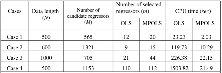
Notice that, for the same problem, MPOLS may select different model terms (regressors) and different

numbers of model terms compared with OLS even for the same threshold value of termination. It is nearly

always true that the MPOLS selects more model terms than that of OLS. However, the first term selected by

both algorithms is always the same. The computational efficiency of the MPOLS algorithm compared with OLS

can be demonstrated using the CPU time required to perform a bench test example on the same computer. This is

[image:16.595.104.487.87.213.2]

Table 1 The comparison of the computational efficiency between OLS and MPOLS

Number of selected

regressors (m) CPU time (sec) Cases Data length

(N)

Number of candidate regressors

(M) _{OLS MPOLS OLS MPOLS}

Case 1 500 565 12 20 23.23 2.03

Case 2 600 1321 9 15 119.73 10.29

Case 3 1000 705 21 44 226.38 22.15

Case 4 500 1153 110 112 1503.82 21.49

Note: The threshold values to terminate the OLS and MPOLS algorithms were the same.

5. Implementing a WANARMAX Model

This section summarizes the procedure for implementing a WANARMAX model. The implementation of a

WANARMAX model involves several practical issues including observational input-output data pre-processing,

significant variable selection (Wei and Billings 2004), resolution level determination in the wavelet

decomposition submodels, and model validity tests (Billings and Voon, 1986; Billings and Zhu, 1995).

The iterative identification procedure to implement a WANARMAX model consists of the following steps.

Step 1: Data pre-processing

For convenience of implementation, convert the original observational input-output data u(t) and y(t)

(t=1,2, …,N) into unit intervals [0,1]. The converted input and output are still denoted by u(t) and y(t).

Step 2: Determining the model initial conditions

This includes:

(i) Provide values for

n

y,

n

u,

n

e,

ρ

and

ρ

e(where

ρ

and

ρ

e are threshold values for terminating the model term selection procedure,

ρ

is used in Step 3 and

ρ

_e in Step 4, notice in general

ρ

_e<

ρ

).

(ii) Set

e

(

t

)

=0 for t=1,2,…,N.

(iii) If possible, select the significant variables from all the candidate lagged output and input variables

{

y

(

t

−

1

),

L

,

y

(

t

−

n

y

),

u

(

t

−

1

),

L

,

u

(

t

−

n

u

)}

. This involves the model order determination and

variable selection problems.

(iv) Select a polynomial submodel

f

P

( t

x

(

))

, a wavelet submodel

f

W

( t

x

(

))

, and a noise model

f

E

(

ξ

(

t

))

from the representations (15)-(17).

(v) Determine the initial and the highest resolution scales. Generally the initial resolution scales

j

₁and

j

₂ in the wavelet models can be set to

j

₁

=

j

₂=0, and the highest resolution scales

J

₁ and

J

₂ can be chosen in a heuristic way.

Step 3: Identify the WANARX model

(i) Calculate the regressors

p

iP

(t

)

and

p

(t

)

( W