This is a repository copy of Posterior mean and variance approximation for regression and
time series problems.
White Rose Research Online URL for this paper:
http://eprints.whiterose.ac.uk/10624/
Article:
Triantafyllopoulos, K. and Harrison, P.J. (2008) Posterior mean and variance
approximation for regression and time series problems. Statistics, 42 (4). pp. 329-350.
ISSN 0233-1888
https://doi.org/10.1080/02331880701864978
[email protected] https://eprints.whiterose.ac.uk/
Reuse
Unless indicated otherwise, fulltext items are protected by copyright with all rights reserved. The copyright exception in section 29 of the Copyright, Designs and Patents Act 1988 allows the making of a single copy solely for the purpose of non-commercial research or private study within the limits of fair dealing. The publisher or other rights-holder may allow further reproduction and re-use of this version - refer to the White Rose Research Online record for this item. Where records identify the publisher as the copyright holder, users can verify any specific terms of use on the publisher’s website.
Takedown
If you consider content in White Rose Research Online to be in breach of UK law, please notify us by
arXiv:0802.0213v1 [stat.ME] 1 Feb 2008
Posterior mean and variance approximation for regression and
time series problems
K. Triantafyllopoulos∗ P.J. Harrison† February 5, 2008
Abstract
This paper develops a methodology for approximating the posterior first two moments of the posterior distribution in Bayesian inference. Partially specified probability mod-els, which are defined only by specifying means and variances, are constructed based upon second-order conditional independence, in order to facilitate posterior updating and prediction of required distributional quantities. Such models are formulated particularly for multivariate regression and time series analysis with unknown observational variance-covariance components. The similarities and differences of these models with the Bayes linear approach are established. Several subclasses of important models, including regres-sion and time series models with errors following multivariate t, inverted multivariate t
and Wishart distributions, are discussed in detail. Two numerical examples consisting of simulated data and of US investment and change in inventory data illustrate the proposed methodology.
Some key words: Bayesian inference, conditional independence, regression, time series, Bayes linear methods, state space models, dynamic linear models, Kalman filter, Bayesian forecasting.
1
Introduction
Regression and time series problems are important problems of statistical inference, which appear widely in many science fields, as for example in econometrics and in medicine.
Re-gression has been discussed in many textbooks (Mardia et al., 1979, Chapter 6; Srivastava
and Sen, 1990); from a Bayesian standpoint Tiao and Zellner (1964), Box and Tiao (1973), Mouchart and Simar (1984), Pilz (1986), Leonard and Hsu (1999, Chapter 5) and O’Hagan and Forster (2004, Chapter 9) discuss a variety of parametric regression models, where the
residuals follow normal or Student t distributions. Recent work on non-normal responses
includes regression models in the type of generalized linear models (GLMs) (McCullagh and Nelder, 1989) and time series models in the type of dynamic GLMs (Fahrmeir and Kaufmann, 1987, 1991; Fahrmeir, 1992; West and Harrison, 1997, Chapter 12; Fahrmeir and Tutz, 2001, Chapter 8; Kedem and Fokianos, 2002; Godolphin and Triantafyllopoulos, 2006). Hartigan (1969) and Goldstein (1976) develop Bayesian inference for a general class of linear regres-sion problems, in which the parameters or states of the regresregres-sion equation are estimated
∗Department of Probability and Statistics, Hicks Building, University of Sheffield, Sheffield S3 7RH, UK,
email: [email protected]
†
by minimizing the posterior expected risk. Goldstein (1979, 1983), Wilkinson and Goldstein (1996) and Wilkinson (1997) propose modifications to the Bayes linear estimators to allow for variance estimation in regression and time series problems. Such considerations are useful in practice because they allow inference to a range of problems that otherwise the modeller would need to resort to Monte Carlo estimation (Gamerman, 1997) or to other simulation based methods (Kitagawa and Gersch, 1996). West and Harrison (1997, Chapter 4) and Wilkinson (1997) discuss how the above mentioned regression estimation can be applied to a sequential estimation problem, which is necessary to consider in time series analysis.
In this paper we propose a modelling framework that allows approximate calculation of the first two moments of the posterior distribution in Bayesian inference. This is motivated by situations when a model may be partially specified in terms of its first two moments, or its probability distribution may be difficult to specify (or it may be specified with uncertainty). Partially specified prior posterior (PSPP) models are developed for dynamic situation in which a modeller is reluctant to specify a full probability model and yet requires a facility for approximate prior/posterior updating on mean and variance/covariance components of
that model. The basic idea is that a linear function φ(X, Y) of two random vectors, X, Y,
is second-order independent of the observed value of Y. Then in learning, no matter what
value ofY is observed, the mean and the variance ofφ(X, Y) takes exactly the same value. A
further requirement is that the mean and variance of X|Y =y can be deduced by the mean
and variance ofφ(X, Y). We show that for a class of regression models, linear Bayes methods
are equivalent to PSPP, while we describe situations where PSPP can provide more effective estimation procedures than linear Bayes. We then describe two wide classes of regression and time series models, the scaled observational precision (SOP) and the generalized SOP, both of which are aimed at multivariate application. For the former model, we give the correspondence of PSPP (based on specification of prior means and variances only) with the normal/gamma model (based on specification of the prior distribution as normal/gamma). For the latter model, we show that PSPP can produce efficient estimation, overcoming problems of existing time series models. This relates to covariance estimation for multivariate state space models when the observation covariance matrix is unknown. For this interesting model we present two numerical illustrations, consisting of simulated bivariate data and of US investment and change in inventory data.
The paper is organized as follows. PSPP models are defined in Section 2. Sections 3 and 4 apply PSPP modelling to regression and time series problems. The numerical illustrations are given in Section 5. Section 6 gives concluding comments and the appendix details the proof of a theorem of Section 2.
2
Partially specified probability modelling
2.1 Full probability modelling
In Bayesian analysis, a full probability model for a random vector Z comprises the joint
dis-tribution of all its elements. The forecast disdis-tribution of any function of Z is then just that
function’s marginal distribution. Learning or updating simply derives the conditional
distri-bution of Z given the received information on the appropriate function of Z. For example,
let Z = [X′ Y′]′, where X, Y are real valued random vectors, and the probability density
function of Z be denoted by p(.). X will often be the vector comprising the parameters or
model is precisely defined, if a density ofY given X is specified, e.g. p(Y|X) so that p(y|X)
is the likelihood function of X based on the single observation Y = y. Then the one-step
forecast distribution ofY is the marginal distribution ofY
p(Y) =
Z
S
p(X, Y)dX, (1)
whereS is the space ofX, also known as parametric space. When the valueyofY is observed,
the revised density of X is
p(X|Y =y) =p(y|X)p(X)
p(y) , (2)
from direct application of the Bayes theorem.
Most Bayesian parametric regression and time series models (including linear and non-linear) adopt the above model structure and their inference involves the evaluation of integral (1) and the Bayes rule (2).
However, in many situations, the evaluation of the above integral is not obtained in closed form and the application of rule (2) does not lead to a conjugate analysis, which is usually desirable in a sequential setting such as for time series application. For such situations, it is
desirable to approximate only the mean and variance of X|Y =y. In this paper we consider
the general problem of obtaining approximations of the first two moments of X|Y =y, when
we only specify the first two moments of X and Y alone and not their joint distribution. We
achieve this by replacing the full conditional independence structure, which is based on the
joint distribution of X and Y, by second order independence, which is based on means and
variances of X and Y. Our motivation is generated from the Gaussian case; suppose thatX
and Y have a joint normal distribution, thenX−AxyY and Y are mutually independent and
the distribution of X|Y =y can be derived from the distribution of X−AxyY, whereAxy is
the regression matrix of X on Y (for a definition of Axy see Section 2.2). So we can define
a subclass of the Bayesian models of (1) and (2), where we can replace the strict mutual independence requirement by second order independence. Details appear in our definition of prior posterior probability models that follow.
2.2 Posterior mean and variance approximation
Let X ∈ Rm, Y ∈ Rp, W ∈ Rq be any random vectors with a joint distribution (m, p, q ∈
N− {0}). We use the notation E(X) for the mean vector of X, Var(X) for the covariance
matrix of X and Cov(X, Y) for the covariance matrix of X and Y. We use the notation
X⊥2Y to indicate that X and Y are second order independent, i.e. E(X|Y = y) = E(X)
and Var(X|Y = y) = Var(X), for any value y of Y. Furthermore, we use the notation
X⊥2W|Y to indicate that, given Y, X and W are second order independent, i.e. E(X|W =
w, Y = y) = E(X|Y = y) and Var(X|W = w, Y = y) = Var(X|Y = y). Details on
conditional independence can be found in Whittaker (1990) or Lauritzen (1996), who discuss independence in a much more sophisticated level necessary for the development of graphical models.
Considering vectors X and Y as above, it is well known that X − AxyY and Y are
uncorrelated, where Axy = Cov(X, Y){Var(Y)}−1 is the regression matrix of X on Y. In
order to obtain approximations of the posterior meanE(X|Y =y) and the posterior covariance
matrix Var(X|Y =y) it is necessary to go one step further and assume that
which of course implies that X −AxyY and Y are uncorrelated. With µx = E(X) and
µy =E(Y), the prior means of X and Y, respectively, the above assumption is equivalent to
the following two postulates.
1. GivenY, the posterior meanE(X−AxyY|Y =y) of X−AxyY does not depend on the
value ofyofY, so that the value of this mean must be the same for all values ofY, and
so be equal to its prior expectation µx−Axyµy.
2. Given Y, the posterior covariance matrix Var(X−AxyY|Y = y) of X−AxyY does
not depend on the value y of Y, so that this posterior covariance matrix takes the
same value for all values y of Y and is necessarily equal to its prior covariance matrix
Var(X−AxyY).
Thus it is possible to approximate E(X|Y =y) and Var(X|Y =y), since from the definition
of second order independence (given above), we have
E(X−AxyY|Y =y) =E(X−AxyY)⇒E(X|Y =y)−Axyy=µx−Axyµy ⇒E(X|Y =y) =µx−Axy(y−µy),
Var(X|Y =y) = Var(X−AxyY|Y =y) = Var(X−AxyY)
= Σx+AxyΣyA′xy−2Cov(X, Y)A′xy = Σx−AxyΣyA′xy
and so we write
X|Y =y∼ {µx+Axy(y−µy),Σx−AxyΣyA′xy},
where Σx= Var(X) and Σy = Var(Y).
Therefore we can define models that have a prior/posterior updating facility that is based on second order independence and that can approximate the posterior mean and variance obtained from an application of the Bayes theorem when the full distributions are specified. Thus we have the following definition.
Definition 1. Let X and Y be any vectors of dimensions m and p respectively and assume that it exists the joint distribution of Z = [X′ Y′]′. Let A
xy be the regression matrix of X
on Y. A first order partially specified prior posterior probability model for (X;Y) (notation: PSPP(1)), is defined such that: (a) X−AxyY⊥2Y and (b) for any value y of Y, the mean vector and the covariance matrix of X|Y = y are obtainable from the mean vector and the covariance matrix of X−AxyY.
We note that ifXandY have a joint normal distribution, then second order independence
is guaranteed and in particular X−AxyY and Y are mutually independent, which is much
stronger than property (3). In this caseE(X|Y =y) and Var(X|Y =y) are the exact posterior
moments, produced by an application of Bayes rule (2). It follows that the approximation of the first two moments reflects on the approximation of postulate (3). Thus the approximations
of E(X|Y =y) and Var(X|Y =y) will be so accurate as the condition (3) is satisfied. The
question is: as we depart from normality, how justified are we to apply (3)? In order to answer this question and to support the adoption of (3), we give the next result, which states that Bayes linear estimation is equivalent to mean and variance estimation employing assumption (3).
The proof of this result is given in the appendix. Thus, if one is happy to accept the assumptions of Bayes linear optimality, she has to employ (3). Next we give three illustrative examples that show assumption (3) may be approximately satisfied.
Example A: checking postulate (3) for the multivariate Student t
distribu-tion
Let X ∈ Rm and Y ∈ Rp be random vectors with a joint Student t distribution with n
degrees of freedom (Gupta and Nagar, 1999,§4.2). For example the marginal density ofX is
the Studenttdistribution X∼ Tm(n, µx, C11) with density function
p(X) = π
−p/2nn/2Γ{(n+p)/2}
Γ(n/2)|C11|1/2
n+ (X−µx)′C11−1(X−µx) (n+p)/2,
for µx =E(X) and Var(X) =nC11/(n−2), where Γ(.) denotes the gamma function and | · |
denotes determinant. Write Z = X Y
∼ Tm+p
n, µx µy ,
C11 C12
C12 C22
,
for some known parameters µx,µy, C11,C12, andC22. The regression coefficient ofX on Y
is Axy =C12C22−1 so that
X−AxyY
Y
∼ Tm+p
n,
µx−Axyµy
µy
,
C11−AxyC22A′xy 0
0 C22
.
Now for any value y of Y, the conditional distribution ofX−AxyY givenY =y is
X−AxyY|Y =y∼ Tm
n+p, µx−Axyµy,(C11−AxyC22A′xy)
1 +n−1(y−µy)C22−1(y−µy)′ .
Thus for any n >0, E(X−AxyY|Y =y) =E(X−AxyY), while for the variance, for n >2,
it is Var(X−AxyY|Y =y)≈n(n−2)−1(C11−AxyC22Axy′ ) = Var(X−AxyY). For large n
postulate X−AxyY⊥2Y is thought to be satisfactory.
Example B: checking postulate (3) for the inverted multivariate Student t
distribution
The inverted Studenttdistribution is discussed in Dickey (1967), in Gupta and Nagar (1999,
§4.4) and it is generated from a multivariate normal and a Wishart distribution as follows.
Suppose thatX∗ ∼ Np(0, Ip) and Σ∼ Wp(n+p−1, Ip), for somen >0, whereWp(n+p−1, Ip)
denotes a Wishart distribution with n+p−1 degrees of freedom and parameter matrixIp;
this distribution belongs to the orthogonally invariant and residual independent family of
distributions, discussed in Khatrie et al. (1991) and Gupta and Nagar (1999, §9.5). For a
vector µand a covariance matrixCwe defineX =n1/2C1/2{Σ +X∗(X∗)′}−1/2X∗+µ, where
C1/2 denotes the symmetric square root ofC. Then the density ofX is
p(X) = Γ{(n+p)/2}
πp/2Γ(n/2)|C|1/2n(p+n−2)/2
n−(X−µ)′C−1(X−µ) n/2−1.
This density defines the inverted multivariate Studenttdistribution and the notation used is
Following a similar thinking as in Example A we have that
X−AxyY ∼ ITm(n, µx−Axyµy, C11−AxyC22A′xy)
and conditioning onY =y (Gupta and Nagar, 1999, §4.4) we obtain
X−AxyY|Y =y∼ ITm{n, µx−Axyµy,(C11−AxyC22A′xy)[1−n−1(y−µy)′C22−1(y−µy)]}.
So we conclude that for largen the mean and variance of X−AxyY|Y = y and X−AxyY
are approximately the same and thusX−AxyY⊥2Y.
Example C: checking postulate (3) for the Wishart distribution
Suppose that Σ = (Σi,j)i,j=1,2 follows a Wishart distribution Σ∼ W2(n, S) with density
p(Σ) =n2nΓ2(n/2)|S|n/2
o−1
|Σ|(n−3)/2exp
−1
2tr(S
−1Σ)
,
where exp(.) denotes exponent, tr(.) denotes the trace of a square matrix, S = (Sij)i,j=1,2,
n > 0 are the degrees of freedom and Γ2(x) = √πΓ(x)Γ(x −1/2) denotes the bivariate
gamma function. Let X = Σ12 and Y = Σ22 and assume that we observe Y = y so that
E(Y) =nS22≈y. From the expected values of the Wishart distribution (Gupta and Nagar,
1999,§3.3.6), we can write
X Y
∼
n
S12
S22
, n
S11S22+S122 2S12S22
2S12S22 2S222
,
which, with Axy =S12/S22, yields E(X−AxyY) = 0 and Var(X−AxyY) =n(S11S22−S122 ).
From Gupta and Nagar (1999, §3.3.4), the posterior distribution of X|Y =y is X|Y =
y ∼ N {S12y/S22,(S11−S122 /S22)y} leading to E(X −AxyY|Y = y) = 0 = E(X−AxyY)
and Var(X−AxyY|Y = y) = Var(X|Y = y) = (S11−S212/S22)y = (S11S22−S122 )y/S22 =
Var(X−AxyY). Thus we can establish that X−AxyY⊥2Y.
Examples A and B show that PSPP(1) modelling can be regraded as approximation to the true posterior mean and variance, corresponding to the full probability model assuming the distribution of these examples.
Returning to Definition 1, there are situations where the prior mean vectors and covariance
matrices ofXandY are available, conditional on some other parameters, the typical example
being when the moments of X and Y are given conditional on a covariance matrixV. Then,
as V is usually unknown, the purpose of the study is to approximate the posterior mean
vector and covariance matrix of X|Y = y as well as to approximate the posterior mean
vector and covariance matrix of V. In such situations postulate (3) reads X−AxyY⊥2Y|V
and another postulate for V is necessary in order to approximate the moments of X|Y =y,
unconditionally of V. Regression problems of this kind are met frequently in practice, as V
can represent an observation variance or volatility, which estimation is beneficial to accounting for the uncertainty of predictions. We can then extend Definition 1 to accommodate for the
Definition 2. Let X, V and Y be any vectors of dimensions m, r and p respectively and assume that it exists the joint distribution ofZ = [X′ V′ Y′]′. LetA
xy be the regression matrix
of X on Y, given V and let Bvy the regression matrix of V on Y. A second order partially
specified prior posterior probability model for(X, V;Y) (notation: PSPP(2)), is defined such that: (a)X−AxyY⊥2Y|V andV −BvyY⊥2Y and (b) for any valuey of Y, the mean vector and the covariance matrix of X|V, Y =y and V|Y =y are obtainable from the mean vector and the covariance matrices of X−AxyY and V −BvyY, respectively.
An example of PSPP(2) model is the scaled observational precision model, which is ex-amined in detail in Sections 3 and 4. Next we discuss the differences of PSPP(2) and Bayes
linear estimation whenV is a scalar variance.
Goldstein (1979, 1983), Wilkinson and Goldstein (1996) and Wilkinson (1997) examine some variants of this problem by considering variance modifications of the basic linear Bayes rule, considered in Hartigan (1969) and in Goldstein (1976). Below we give a basic description of the proposed estimators and we indicate the similarities and the differences of the proposed PSPP models and of the Bayes linear estimators. Consider a simple regression problem
formulated asY|X, V ∼(X, V),X ∼ {E(X),Var(X)}, whereY is a scalar response variable,
X is a scalar regressor variable and E(X), Var(X) are the prior mean and variance of X. If
V is known the posterior meanE(X|V, Y =y) can be approximated by the Bayes linear rule
µ= E(X)V +yVar(X)
V + Var(X) =E(X) +Axy{y−E(X)}, (4)
with related posterior expected risk
R(µ) = Var(X)V
Var(X) +V = Var(X)(1−Axy),
whereAxy = Var(X)/{Var(X) +V}is the regression coefficient ofX onY, conditional onV.
As it is well known R(µ) is the minimum posterior expected risk, over all linear estimators
for E(X|Y = y), and in this sense µ attains Bayes linear optimality. If one assumes that
the distributions ofY|X, V and X are normal distributions, thenµgives the exact posterior
mean E(X|V, Y =y) andR(µ) gives the exact posterior variance Var(X|V, Y =y). However,
in practice in many problems, V is not known, and ideally the modeller wishes to estimate
V and provide an approximation to the mean and variance of X|Y = y, unconditionally of
V. Suppose that in addition to the above modelling assumptions, in order to estimate V, a
prior meanE(V) and prior variance Var(V) ofV are specified, namelyV ∼ {(E(V),Var(V)}.
Goldstein (1979, 1983) suggest to estimate V with the Bayes linear rule
V∗ = E(V)Var(Y
∗) +y∗Var(V)
Var(Y∗) + Var(V) , (5)
wherey∗ is an observation fromY∗, a statistic that is unbiased forV, and Var(Y∗) is specified
a priori. Then the Bayes rule µ is replaced by the rule µ∗, whereV in µ is replaced by its
estimateV∗. One can see that the revised regression matrix A∗
xy becomes
A∗xy = Var(X)
Var(X) +V∗ =
Var(X)Var(Y∗) + Var(X)Var(V)
Var(X)Var(Y∗) + Var(X)Var(V) +E(V)Var(Y∗) +y∗Var(V)
and so the variance modified Bayes rule for E(X|Y =y) is µ∗ =E(X) +A∗
From Theorem 1, it is evident that the Bayes rule (4) is equivalent to X−AxyY⊥2Y|V.
The Bayes rule (5) corresponds to the postulateV −BvyY⊥2Y, although the latter does not
establish the equivalence of the PSPP models and Bayes linear estimation methods, since it
can be verified that µ∗ and V∗ are not the same as in the PSPP modelling approach (see
Section 3). In addition, the roles of Y∗ and y∗ are not fully understood; for example one
question is howy and y∗ are related and how one can determiney∗ from y, especially when
y is a vector of observations. The main problem experienced in the variance modified Bayes
linear estimator µ∗ is that the related expected risk R(µ∗) can not easily be determined
and the work in this direction (Goldstein, 1979, 1983) has led to either intuitive evaluation
for R(µ∗) or it has led to imposing even more restrictions to the model in order to obtain
an analytic formula for R(µ∗). Although, both of these approaches can work in regression
problems, they are not appropriate for time series problems, where sequential updating is required and thus an accurate evaluation of that risk is necessary. On the other hand the
PSPP approach combines the two postulates, X−AxyY⊥2Y|V and V −BvyY⊥2Y, using
conditional expectations. It should be noted that the PSPP treatment is free of most of the assumptions made to the variance modified Bayes linear system so that approximate
estimation of the posterior Var(X|Y) be given. The PSPP models are developed mainly
for multivariate regression and time series problems and they are aimed to situations that either a fully Bayesian model is not available, or computationally intensive calculations, such as Monte Carlo methods, are undesirable, or a model can only be specified via means and variances.
3
The scaled observational precision model
3.1 Main theory
The scaled observational precision (SOP) model is a conjugate regression model, which illus-trates the normal dynamic linear model with observational variances, see for example West
and Harrison (1997,§4.5). This model is widely used in practice because it is capable to
han-dle the practical problem of unknown observation variances. Here we construct a PSPP(2) model and we compare it with the usual conjugate SOP model.
LetV be a scalar variance, X∈Rm,Y ∈Rp with
Z =
X
Y V ∼
µx
µy
, V
Σx AxyΣy
AyxΣx Σy
,
for some knownµx,µy, Σx and Σy.
AssumingX−AxyY⊥2Y|V, the partially specified posterior is
X|V, Y =y∼ {µx+Axy(y−µy), V(Σx−AxyΣyA′xy)}.
LetT be a, generally non-linear, function of Y, often taken as
T = (Y −µy)′Σy−1(Y −µy).
DefineK to be aα times the variance ofT|V, for someα >0, and Avτ to be the regression
coefficient of V on T, conditional onK. We assume V −AvτT⊥2Y, K with forecast
where V|K ∼ (V , K/ηb ), which is η/α times as precise as the conditional distribution of T,
for some knownV , α, ηb , with
V T K∼ (" b V b V # ,K η 1 1
1 (η+α)/α
)
.
Given the observation T =τ, and usingV −AvτT⊥2Y, K withAvτ =α/(η+α) we have
E(V|K, T =τ) =E(V|K) + α
η+α[τ −E(T|K)] =
ηVb +ατ η+α ,
Var(V|K, T =τ) = Var(V|T =τ)−Cov(V, T|K){Var(T|K)}−1Cov(T, V|K)
= K
η − K2
η2
ηα K(η+α) =
K η
1− α
η+α
= K
η+α
so that
V|K, T =τ ∼ ηVb +ατ η+α ,
K η+α
!
. (6)
Hence using conditional expectations, it follows that
X|Y =y∼
(
µx+Axy(y−µy),
ηVb+ατ
η+α (Σx−AxyΣyAyx)
)
, (7)
where τ = (y−µy)′Σ−y1(y−µy).
3.2 Comparison with the conjugate normal/gamma model
Now consider the relationship of the above model with standard normal conjugate models. A
typical normal conjugate model with unknown scalar varianceV, postulates the distribution
of Z given V as
Z = X Y
V ∼ Nmp
µx µy , V
Σx AxyΣy
AyxΣx Σy
,
with the distribution of V as an inverse gamma so that νs/V ∼χ2
ν. Here Nmp(., .) denotes
the mp-dimensional normal distribution and χ2ν denotes the chi-squared distribution with ν
degrees of freedom. Writing T = (Y −µy)′Σy−1(Y −µy), the conditional distribution of T
given V can be easily derived from the distribution ofT V−1|V which isT V−1|V ∼χ2
p. Then
the posterior distribution ofV−1 given Y =y is
p 1 V
T =τ
= p(τ|V)p(1/V)
p(τ) ∝
1
V
(ν+p)/2−1
exp
−νs+τ
2V
,
from which it is deduced that, given Y = y, (νs+τ)V−1|Y = y ∼ χ2
ν+p. The posterior
distribution of X|Y =y is a multivariate Student tdistribution based uponν+pdegrees of
freedom with
X|Y =y∼ Tm
ν+p, µx+Axy(y−µy),
νs+τ
ν+p (Σx−AxyΣyAyx)
, (8)
νs+τ V
Note that, ifVb =νs/(ν+p−3), η =ν+p−3, and α = 1, then the posterior mean vector and covariance matrix of (7) and (8) are identical. However, this is not consistent with the
conjugate model since from the prior assumptionνs/V ∼χ2ν it is
E(V|s) = νs
ν−2 6=V ,b (ν >2),
for any p >1.
If we want to adopt the same prior forVb =νs/(ν−2) in both the PSPP and the conjugate
models, then the respective posterior means forV will differ, i.e.
E(V|Y =y,PSPP model)−E(V|Y =y,conjugate model) = (p−1)νs
(ν−2)(ν+p−2),
where we have usedη=ν+p−3 andα= 1 as before. Note that ifY is a scalar response, e.g.
p= 1, then the two variance estimates are identical. So the respective posterior variances of
equations (7) and (8) will differ accordingly only when p >1.
From the posterior distribution of 1/V we have that
Var(V|Y =y,conjugate model) = 2(τ +νs)
2
(ν+p−2)2(ν+p−4) (10)
while, from equation (6), the respective posterior variance for the PSPP model is
Var(V|K, Y =y,PSPP model) = K
ν+p−2, (11)
where we have usedα= 1 andη =ν+p−3. If we chooseK = 2(τ+νs)2/{(ν+p−2)(ν+p−4)},
then the two variances will be the same. Note that, irrespectively of the choice of K (given
that K is bounded), as the degrees of freedom ν tend to infinity, the variances of both
equations (10) and (11) converge to zero and so as ν → ∞, V concentrates about its mean
asymptotically degenerating.
3.3 Application to time series modelling I
The above ideas can be applied to time series modelling when interest is placed on the
estima-tion of the observaestima-tion or measurement variance. Consider, for example, the p-dimensional
time series vector Yt, which at a particular timetsets
Yt=BtXt+ǫt, ǫt∼(0, V Z), Xt=CtXt−1+ωt, ωt∼(0, V W), (12)
where Bt is a known p×m design matrix, Ct is a known m×m transition matrix and the
innovation error sequences {ǫt} and {ωt} are individually and mutually uncorrelated. The
p×pand m×m covariance matricesZ andW are assumed known, while the scalar variance
V is unknown. Initially we assume
X0|V ∼(m0, V P0) and V ∼
b
V0,
K0
η0
,
for some knownm0,P0,Vb0,K0andη0. It is also assumed thata priori,X0is uncorrelated with
Then the PSPP model described above, applies at each time twithµx =Ctmt−1,µy =ft=
BtCtmt−1, Σx =Rt=CtPt−1Ct′+W and Σy =Qt=BtRtBt′+Z, wheremt−1 and Pt−1 are
calculated with the same way at timet−1, starting with t= 1. Given yt−1, the regression
matrix of Xt on Yt is Axy = At = RtBt′Q−t1, which is independent of V. It follows that
V|yt∼(Vbt, Kt/ηt). With α= 1, it isKt=Kt−1 and ηt=ηt−1+ 1 so that
ηtVbt=ηt−1Vbt−1+e′tQ−t1et,
wheree′
tQ−t1et= τt and et =yt−ft is the 1-step forecast error vector. The above estimate
b
Vt approximates the variance estimate of the conjugate dynamic linear model (West and
Harrison, 1997, §4.5), which, assuming a prior ηt−1Vbt−1V−1|yt−1 ∼ χ2ηt−1, arrives at the
posterior (ηt−1Vbt−1 +τt)V−1|yt ∼ χ2ηt−1+p so that E(V|y
t) = η
tVbt/(ηt+p−3) ≈ Vbt. The
variance of V|ytin the conjugate model is
Var(V|yt) = 2η
2 tVbt2
(ηt−2)2(ηt−4)
,
whereas the respective variance in the PSPP model is Var(V|yt) = K/ηt, with K = K0.
Although these two variances differ considerably, in the sense that in the conjugate model the
variance of V|yt is a function of the data yt and in the PSPP model the variance ofV|yt is
only a function of time t and on the prior K0, it can be seen that ast→ ∞, both variances
converge to zero and so in both cases V|yt concentrates about its mean Vbt asymptotically
degenerating.
In the PSPP model, the posterior mean vector and covariance matrix of Xt|yt are given
by Xt|yt∼(mt,VbtPt), wheremt=Ctmt−1+Atetand Pt=Rt−AtQtA′t. These approximate
the respective mean vector and covariance matrix produced by the conjugate model, which,
under the inverted gamma prior, results to the posterior Student t distribution: Xt|yt ∼
Tm(ηt, mt,VbtPt).
4
The generalized observational precision model
4.1 Main theory
The generalization of the SOP model of Section 3 when V is a p×p variance-covariance
matrix is not available and only special forms of conjugate SOP models are known (West
and Harrison, 1997, Chapter 16). The problem is that since the dimensions of X and Y
are different, it is not possible to scale the covariance matrix of X|V by V, because X has
dimension m and V is a p×p matrix. This problem is discussed in detail in Barbosa and
Harrison (1992) and Triantafyllopoulos (2007). Next we propose a generalization of the SOP
model, in which, given V, we avoid to scale the covariance matrices of X and Y by V.
This setting is more natural than the setting of the SOP, which considers the somewhat mathematically convenient variance scaling.
LetV be a p×p covariance matrix, X∈Rm,Y ∈Rp with
Z=
X Y
V ∼
µx
µy
,
Σx Axy(Σy+V)
(Σy +V)A′xy Σy+V
,
for some known µx, µy, Σx and Σy, not depending onV. Note that now we cannot gain a
obtain the marginal distributionsX|Y =y andV|Y =y in closed form, since the covariance
matrices of X and Y are not scaled by V.
AssumingX−AxyY⊥2Y|V, conditional onV, the partially specified posterior is
X|V, Y =y∼ {µx+Axy(y−µy),Σx−Axy(Σy +V)−1A′xy}. (13)
DefineT = (Y−µy)(Y −µy)′−Σy and denote with vech(V) the column stacking operator
of a lower portion of the symmetric positive definite matrixV. Given V, the forecast ofT is
vech(T)|V, K∼
vech(V),K
α
and
Cov{vech(V),vech(T)}= K
η = Var{vech(V|K)},
whereα,η are known positive scalars andKis a known{p(p+1)/2}×{p(p+1)/2}covariance
matrix. WithVb the prior estimate ofV andIp(p+1)/2 the{p(p+ 1)/2} × {p(p+ 1)/2}identity
matrix, we have
vech(V)
vech(T)
K∼
("
vech(Vb)
vech(Vb)
#
,K η
Ip(p+1)/2 Ip(p+1)/2 Ip(p+1)/2 (η+α)α−1I
p(p+1)/2
)
.
The regression matrix of vech(V) on vech(T) isAvτ =α(η+α)−1Ip(p+1)/2. Assuming now
that vech(V)−Avτvech(T)⊥2T|K we obtain the posterior mean and covariance of V as
E{vech(V)|K, T =τ}= vech(Vb) + α
η+α
n
vech(τ)−vech(Vb)o
and
Var{vech(V)|K, T =τ}= Var{vech(V)|K}+AvτVar{vech(T)|K}A′vτ =
K η+α
so that
vech(V)|K, T =τ ∼
(
vech(ηVb +ατ)
η+α , K η+α
)
, (14)
from which we see that the posterior mean ofV can be written as
E(V|K, T =τ) =Vb + α
η+α
τ−Vb= ηVb +ατ
η+α .
We note that in general the regression matrix Axy in (13) will be a function ofV−1 and this
adds more complications to the calculation of the mean and covariance matrix of X|Y =y.
However, if we impose the assumption that Cov(X, Y|V) = AVar(Y), where A is a known
m×p matrix not depending onV, then Axy =A is independent of V and so we get
X|Y =y∼
µx+Axy(y−µy),Σx− 1
η+αAxy
Σy+ηVb +ατA′xy
, (15)
whereτ = (y−µy)(y−µy)′−Σy. Given thatKis bounded, as η→ ∞, the covariance matrix
of vech(V)|K, T =τ converges to the zero matrix and so V|K, T =τ concentrates about its
meanE(V|K, T =τ) asymptotically degenerating. This can be a theoretical validation of the
proposed procedure for the accuracy of the estimator ofV,E(V|K, T =τ) = (ηVb+ατ)/(η+
4.2 Application to linear regression modelling
A typical linear regression model sets
Y =BX+ǫ, ǫ∼(0, V), X ∼(µx,Σx), (16)
whereY is ap-dimensional vector of response variables,B is a knownp×mdesign matrix and
ǫis ap-dimensional error vector, which is uncorrelated with the randomm-dimensional vector
X. The mean vector µx and the covariance matrix Σx are assumed known and Σy =BΣxB′
so that Var(Y) =BΣxB′+V. The covariance matrix ofX and Y is Cov(X, Y) = ΣxB′ and
so the assumption Cov(X, Y) =A{Var(Y)}−1, does not hold, since Var(Y) is a function ofV.
Thus the posterior mean vector and covariance matrix of equation (15) do not apply, since now
Axy is stochastic in V. In order to resolve this difficulty next we propose an approximation
that will allow computation of equation (13).
In order to proceed, we will need to evaluate E{(Σy+V)−1|Y =y} and Var{vech{(Σy+
V)−1}|Y =y}. Since we only have equation (14) and we have no information on the
distribu-tion ofV, we can not obtain the above mean vector and covariance matrix. Here we choose
to adopt an intuitive approach suggesting that
e
V = E{(Σy+V)−1|K, T =τ} ≈ {Σy+E(V|K, T =τ)}−1
= (η+α)n(η+α)Σy+ηVb +ατ
o−1
,
ee
V = Var[vech{(Σy+V)−1}|K, T =τ]≈Var{vech(Σy+V)|K, T =τ}= K
η+α.
The reasoning of this is as follows. Since limη→∞Var{vech(V)|K, T =τ}= 0,V concentrates
about its mean and so we can write V ≈ E(V|K, T = τ), for sufficiently large η. Then
(Σy +V)−1 ≈ {Σy +E(V|K, T = τ)}−1. The covariance matrix of vech{(Σy +V)−1} has
been set approximately the same with the covariance matrix of vech(Σy +V) ensuring that
for largeη, both covariance matrices converge to zero.
The above problem of the specification ofVe and Vee can be generally presented as follows.
Suppose that M is a bounded covariance matrix and assume thatE(M) and Var{vech(M)}
are finite and known. The question is, given only this information, can one obtain E(M−1)
and Var{vech(M−1)}? For example one can notice that if M follows a Wishart or inverted
Wishart distributions, thenVe is approximately true. Formally, ifM ∼ Wp(n, S) (M follows
the Wishart distribution withndegrees of freedom and parameter matrix S, see e.g. Gupta
and Nagar, 1999, Chapter 3), we have E(M) = nS and E(M−1) = S−1/(n−p−1) =
n{E(M)}−1/(n−p−1), which impliesE(M−1)≈ {E(M)}−1, for largen. IfM ∼ IWp(n, S)
(M follows the inverted Wishart distribution withndegrees of freedom and parameter matrix
S, see e.g. Gupta and Nagar, 1999, Chapter 3), we have E(M) = S/(n−2p −2) and
so E(M−1) = (n−p−1)S−1 = (n−p−1){E(M)}−1/(n−2p−2), which again implies
E(M−1)≈ {E(M)}−1, for largen. Of courseM might not follow Wishart of inverted Wishart
distributions and in many practical situations we will not have access to the distribution of
M. For general application we can verify that E(M−1) ≈ {E(M)}−1, if and only if M and
M−1 are uncorrelated. The accuracy of the choice of Ve is reflected on the accuracy of the
one-step predictions, which is illustrated in Section 5.1.
We can now apply conditional expectations to obtain the mean vector and the covariance
matrix ofX|Y =y. Indeed from the above and equation (13) we have
For the covariance matrix Var(X|Y =y) we have
E{Var(X|V, Y =y)|Y =y} = Σx−ΣxB′E{(Σ +V)−1|Y =y}BΣx
= Σx−ΣxB′V Be Σx
and
Var{E(X|V, Y =y)|Y =y} = Var[vec{ΣxB′(Σy+V)−1(y−µy)}|Y =y]
= {(y−µy)′⊗ΣxB′}GpV Gee ′p{(y−µy)⊗BΣx}.
where ⊗ denotes Kronecker product, vec(·) denotes the column stacking operator of a lower
portion of a matrix andGpis the duplication matrix, namely vec{(Σy+V)−1}=Gpvech{(Σy+
V)−1}.
Thus the mean vector and the covariance matrix ofX|Y =y are
X|Y =y ∼ nµx+ ΣxB′Ve(y−µy),Σx−ΣxB′V Be Σx
+[(y−µy)′⊗ΣxB′]GpV Gee ′p[(y−µy)⊗BΣx]
. (17)
We note that the mean vector and covariance matrix of X|Y = y depend on the estimates
e
V and Vee. A simple intuitive approach was employed in this section and next we give an
assessment of this approach by simulation. In general, equation (17) holds where Ve and Vee
are any estimates of the mean vector and covariance matrix of (Σy+V)−1|Y =y.
4.3 Application to time series modelling II
In this section we consider the state space model (12), but the covariance matrices of the error
driftsǫt and ωt are Var(ǫt) =V and Var(ωt) = W. Here V is an unknownp×p covariance
matrix andW is a known m×m covariance matrix. The priors are partially specified by
X0∼(m0, P0) and vech(V)∼
vech(Vb0),
K0
η0
,
for some knownm0, P0, Vb0, K0 and η0. It is also assumed that a priori, X0 is uncorrelated
with {ǫt} and {ωt}. Note that in contrast with model (12), the above model is not scaled
by V and in fact any factorization of the covariance matrices by V would lead to restrictive
forms of the model; for a discussion of this topic see Harvey (1989), Barbosa and Harrison
(1992), West and Harrison, (1997, §16.4), and Triantafyllopoulos (2006a, 2007). Before we
give the proposed estimation algorithm, we give a brief description of the related matrix-variate dynamic models (MV-DLMs) and the restrictions imposed in these models.
Suppose {Yt} is a p-dimensional vector of observations, which are observed in roughly
equal intervals of time t = 1,2,3, . . .. Write Yt = [Y1t Y2t · · · Ypt]′, where each of Yit is
modelled as a univariate dynamic linear model (DLM):
Yit=Bt′Xit+ǫit, Xit=CtXi,t−1+ωit, ǫit∼ N(0, σii), ωit ∼ Nm(0, σiiWi),
where Bt is an m-dimensional design vector, Xit is an m-dimensional state vector, Ct is
uncorrelated and also they are uncorrelated with the state prior Xi,0, which is assumed to
follow the normal distributionXi,0 ∼ Nm(mi,0, Pi,0), for some knownmi,0andPi,0. Them×m
covariance matrixWi is assumed known and the variancesσ11, σ22, . . . , σpp form the diagonal
elements of the covariance matrix Σ = (σij)i,j=1,2,...,p, which is assumed unknown and it is
subject to Bayesian estimation under the inverted Wishart prior Σ ∼ IWp(n0+ 2p, n0S0),
for some knownn0 and S0. The model can be written in compact form as
Yt′=Bt′Xt+ǫt′, Xt=CtXt−1+ωt, ǫt∼ Np(0,Σ), vec(ωt)∼ Nmp(0,Σ⊗W), (18)
whereB′
t= [B1′tB2′t · · · Bpt′ ],Xt= [X1tX2t · · · Xpt],Ct= diag(C1t, C2t, . . . , Cpt), vec(X0)∼
Nmp{vec(m0),Σ⊗P0}, for m0 = [m1,0 m2,0 · · · mp,0] and P0 = diag(P1,0, P2,0, . . . , Pp,0).
Model (18) is termed as matrix-variate dynamic linear model (MV-DLM) and it is studied in Quintana and West (1987, 1988), Smith (1992), West and Harrison (1997, Chapter 16)
Triantafyllopoulos and Pikoulas (2002), Salvadoret al. (2003, 2004), Salvador and Gargallo
(2004), and Triantafyllopoulos (2006a, 2006b); Harvey (1986, 1989) develop a similar model where Σ is estimated by a quasi likelihood estimation procedure. The disadvantage of model
(18) is that Y1t, Y2t, . . . , Ypt are restricted to follow similar patterns since the model
compo-nentsBt and Ct are common for all i= 1,2, . . . , p. One can notice that the only difference
between Yit and Yjt(i6=j), is due to the error driftsǫit,ωit and ǫjt,ωjt. Thus, for example,
model (18) is not appropriate to modelYt= [Y1tY2t]′, whereY1tis a trend time series andY2t
is a seasonal time series. It follows that when there are structural changes betweenYit and
Yjt, the MV-DLM might be thought of as restrictive and inappropriate model and its use is
not recommended. Whenp is large one can hardly justify the “similarity” ofY1t, Y2t, . . . , Ypt.
We believe that in practice the popularity of the MV-DLM is driven from its mathematical properties (fully Bayesian conjugate estimation procedures for sequential forecasting and fil-tering/smoothing), rather than from a data driven analysis. Although we accept that in some cases the MV-DLM can be a useful model, we would submit that in many time series problems this model is unjustifiable and the above discussion expresses our reluctance in suggesting the MV-DLM for general use for multivariate time series problems.
Returning now to the PSPP dynamic model, denote withytthe information set comprising
data y1, y2, . . . , yt. If at time t−1 the posteriors are partially specified by Xt−1|yt−1 ∼
(mt−1, Pt−1) and vech(V)|yt−1 ∼ {vech(Vbt−1), ηt−−11Kt−1}, for some known mt−1, Pt−1,Vbt−1,
Kt−1 and ηt−1, then by direct application of the theory of Section 4 we have for time t:
µx = Ctmt−1, Σx = Rt = CtPt−1Ct′ +W, µy = ft = BtCtmt−1, Σy = BtRtBt′ and Axy =
At=RtBt′(BtRtBt′+V)−1. The 1-step ahead forecast covariance matrix isQt= Var(Yt|yt) =
BtRtBt′+Vbt−1and so we haveYt|yt−1 ∼(ft, Qt). GivenYt=yt, the error vector iset=yt−ft
and so the posterior mean ofV|yt is
ηtVbt=ηt−1Vbt−1+ete′t−BtRtBt′,
where we have usedα= 1. Thus it is
vech(V)|yt∼
vech(Vbt),
Kt
ηt
,
whereηt =ηt−1+ 1 and Kt =Kt−1. It follows that Kt=K0 and therefore as t→ ∞,V|yt
concentrates about Vbt asymptotically degenerating. By observing that BtRtBt′ =Qt−Vbt−1
and writing the updating ofVbt recurrently, we get
b
Vt=Vbt−1+
ete′t−Qt
ηt
=Vb0+
t
X
i=1
eie′i−Qi
η0+i
By forming now the standardized 1-step ahead forecast errors e∗
t = Q
−1/2
t et, where Q
−1/2 t
denotes the symmetric square root of Q−t1, one can obtain a measure of goodness of fit,
since e∗
t ∼ (0, Ip). This can easily be implemented, by checking whether the mean of
e∗
1(e∗1)′, e∗2(e∗2)′, . . . , e∗t(e∗t)′is close toIpor equivalently by checking that, fore∗t = [e∗1te∗2t · · · e∗pt]′,
the mean of each (e∗
i,1)2,(e∗i,2)2, . . . ,(e∗it)2 is close to 1 ande∗it is uncorrelated withe∗jt, for all
t and i6=j.
Applying the procedure adopted in linear regression, we have that the posterior mean
vector and covariance matrix are given by Xt|yt∼(mt, Pt), with
mt=Ctmt−1+RtBt′Vetet and
Pt=Rt−RtBt′VetBtRt+ (e′t⊗RtBt′)GpVeetG′p(et⊗BtRt), where
e
Vt= (BtRtBt′+Vbt)−1 and Veet=
K0
ηt
.
From ηt = ηt−1+ 1 it follows that as limt→∞ηt = ∞ it is limt→∞Veet = 0 and so for large
t the posterior covariance matrix Pt can be approximated by Pt ≈ Rt−RtBt′VetBtRt. This
can motivate computational savings, since there is no need to perform calculations involving Kronecker products.
5
Numerical illustrations
In this section we give two numerical examples of the state space model considered in Section 4.3.
5.1 A simulation study
We simulate 1000 bivariate time series under 3 state space models and we compare the performance of the proposed model of Section 4.3 (referred here as DLM1), of the MV-DLM discussed in 4.3 (referred here as DLM2) and of the general multivariate dynamic linear model
(referred here as DLM3). LetYt= [Y1tY2t]′ be a bivariate time series. In the first state space
model we simulate 1000 bivariate time series from the model
Yt=
1 0 0 1
Xt+ǫt, Xt=
1 0 0 1
Xt−1+ωt, ǫt∼ N2(0, V), ωt∼ N2(0, I2), (19)
where Xt is a bivariate state vector and the remaining components are as in Section 4.3.
Initially we assume that X0 ∼ N2(0, I2) and the covariance matrixV is
V = (Vij)i,j=1,2 =
1 2 2 5
,
which means that the variables Y1t and Y2t are highly correlated. The generated time series
{Yt} comprise two local level components, namely {Y1t} and {Y2t}. We note that DLM3 is
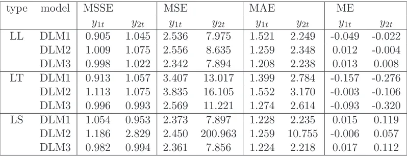
Table 1: Performance of the PSPP dynamic model (DLM1), MV-DLM (DLM2) and the general bivariate dynamic model (DLM3) over 1000 simulated time series of two local level components (LL), one local level and one linear trend component (LT) and one local level and one seasonal component (LS). Shown are the average (over all 1000 simulated series) values of the mean square standard error (MSSE), of the mean square error (MSE), of the mean absolute error (MAE) and of the mean error (ME).
type model MSSE MSE MAE ME
y1t y2t y1t y2t y1t y2t y1t y2t
LL DLM1 0.905 1.045 2.536 7.975 1.521 2.249 -0.049 -0.022
DLM2 1.009 1.075 2.556 8.635 1.259 2.348 0.012 -0.004
DLM3 0.998 1.022 2.342 7.894 1.208 2.238 0.013 0.008
LT DLM1 0.913 1.057 3.407 13.017 1.399 2.784 -0.157 -0.276
DLM2 1.113 1.075 3.835 16.105 1.552 3.170 -0.003 -0.106
DLM3 0.996 0.993 2.569 11.221 1.274 2.614 -0.093 -0.320
LS DLM1 1.054 0.953 2.373 7.897 1.228 2.235 0.015 0.119
DLM2 1.186 2.829 2.450 200.963 1.259 10.755 -0.006 0.057
DLM3 0.982 0.994 2.361 7.856 1.224 2.218 0.017 0.112
In the second state space model we simulate 1000 time series from the model
Yt=
1 0 0 1
Xt+ǫt, Xt=
1 1 0 1
Xt−1+ωt, ǫt∼ N2(0, V), ωt∼ N2(0, I2),
and the remaining components are as in (19). The generated time series from this model are
time series comprising{Y1t}as a local level component and{Y2t}as a linear trend component.
Finally, in the third state space model, we simulate 1000 time series from the model
Yt=
1 0 0 0 1 0
Xt+ǫt, Xt=
1 0 0
0 cos(π/6) sin(π/6)
0 −sin(π/6) cos(π/6)
Xt−1+ωt, (20)
where ǫt ∼ N2(0, V), ωt ∼ N3(0, I3) and here Xt is a trivariate state vector with initial
distributionX0 ∼ N3(0, I3) and the remaining components of the model are as in (19). The
generated time series from this model are bivariate time series comprising {Y1t} as a local
level component and {Y2t} as a seasonal component with period π/3. Such seasonal time
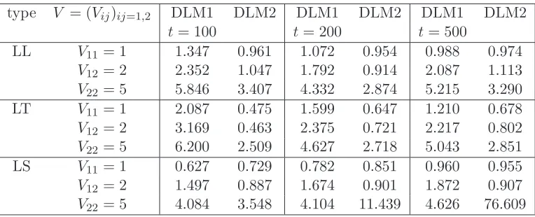
Table 2: Performance of estimators of the covariance matrix V = (Vij)i,j=1,2, produced by the PSPP dynamic model (DLM1) and the MV-DLM (DLM2). Shown are the average (over
all 1000 simulated series; see Table 1) values of each estimator for timest= 100,t= 200 and
t= 500.
type V = (Vij)ij=1,2 DLM1 DLM2 DLM1 DLM2 DLM1 DLM2
t= 100 t= 200 t= 500
LL V11= 1 1.347 0.961 1.072 0.954 0.988 0.974
V12= 2 2.352 1.047 1.792 0.914 2.087 1.113
V22= 5 5.846 3.407 4.332 2.874 5.215 3.290
LT V11= 1 2.087 0.475 1.599 0.647 1.210 0.678
V12= 2 3.169 0.463 2.375 0.721 2.217 0.802
V22= 5 6.200 2.509 4.627 2.718 5.043 2.851
LS V11= 1 0.627 0.729 0.782 0.851 0.960 0.955
V12= 2 1.497 0.887 1.674 0.901 1.872 0.907
V22= 5 4.084 3.548 4.104 11.439 4.626 76.609
Section 4.3 details how the MSSE has been calculated. Out of the three models we know that DLM3 is the correct model, since it is used to generate the time series data. For the local level components (LL), both DLM1 and DLM2 put good performances with the DLM2 having the edge and being closer to the performance of the DLM3. This is expected, since as
we noted in Section 4.3 when both time series components Y1t and Y2t are similar the
MV-DLM (MV-DLM2) has good performance. However, in the LT and LS time series components,
where the two seriesY1tand Y2t in each case, are not similar, we expect that the DLM2 will
not perform very well. This is indeed confirmed by our simulations, for which Table 1 clearly shows that the performance of DLM1 is better than that of the DLM2. For example, for the
LS component, the MSSE of the DLM1 is [1.054 0.953]′, which is close to [1 1]′, while the
respective MSSE of the DLM2 is [1.186 2.829]′.
Table 2 looks at the accuracy of the estimation of the covariance matrixV, for each model.
For the LL components V11 = 1 is estimated better from DLM2, although for t = 500 the
estimate from DLM1 is slightly better. ForV12= 2 andV22= 5, DLM2 produces poor results
as compared to the DLM1. For example, even for t = 500 the estimate of V22 = 5 of the
DLM2 is only 3.290, while the estimate of the DLM1 is 5.215. This phenomenon appears to
be magnified when looking at the LT and LS components, where for example even att= 500
for the LT the estimate of V12 = 2 and for the LS the estimate of V22 = 5 are 0.802 and
76.609, while the respective estimates from the DLM1 are 2.217 and 4.626. The conclusion is that the DLM1 produces a consistent estimation behaviour over a wide range of bivariate time series, while the DLM2 (matrix-variate DLM) produces acceptable performance when the component time series are all similar.
Real data vs 1−step forecasts
year
response
1950 1955 1960 1965 1970
0
50
100
[image:20.612.87.487.140.441.2]150
Figure 1: US Investment and Change in Inventory time seriesyt = [y1t y2t]′ with its 1-step
forecast mean ft = [f1t f2t]′. The top solid line shows y1t and the bottom solid line shows
y2t; the top dashed line shows f1tand the bottom dashed line shows f2t.
space models and for local level models. More general structures, such that of model (20) can only be dealt with via simulation-based methods, such as Monte Carlo simulation. For high-dimensional dynamical systems and in particular for observation covariance estimation, the proposal of PSPP state space model of Section 4.3 offers a fast and reliable approximate estimation procedure, which can be applied for a wide range of time series.
5.2 The US investment and business inventory data
We consider US investment and change in business inventory data, which are deseasonalised
and they are measured quarterly into a bivariate time series (variable y1t: US investment
data and variabley2t: US change in inventory data) over the period 1947-1971. The data are
fully described and tabulated in L¨utkepohl (1993) and Reinsel (1997, Appendix A). The data
Yt=
1 0 0 1
Xt+ǫt, Xt=
1 1 0 1
Xt−1+ωt, ǫt∼(0, V), ωt∼(0, Wt), (21)
where here we have not specified the distributions ofǫtandωtas normal and we have replaced
the time-invariant W of Section 4.3 with a time-dependentWt. Model (21) is a PSPP linear
trend state space model, for which we choose the priors m0 = [80.622 4.047]′ (mean of
[Y1tY2t]′ fort= 1941−1956, indicated in Figure 1 by the vertical line),P0 = 1000I2 (weakly
informative prior covariance matrix or low precision P0−1 ≈0) and
V0 =
66.403 22.239
22.239 46.547
,
which is taken as the sample covariance matrix ofY1t andY2t, for the time period 1941-1955.
The covariance matrixWtmeasures the durability and the stability of the change or evolution
of the states Xt. Here we specify Wt with 2 discount factors, δ1 and δ2, as follows. With G
as the evolution matrix ofXt and ∆ the discount matrix
G=
1 1 0 1
, ∆ =
δ1 0
0 δ2
,
we have
Wt= ∆−1/2GPt−1G′∆−1/2−GPt−1G′,
where Rt in the recursions of Section 4.3 is replaced byRt =GPt−1G′+Wt. Although this
discounting specification is not advocated by West and Harrison (1997, §6.4), it has been
successfully used (McKenzie, 1974, 1976; Abraham and Ledolter, 1983, Chapter 7; Ameen and Harrison, 1985; Goodwin, 1997).
The values of δ1 and δ2 are chosen by experimentation. The above model gave the best
result with a combination of discount factors δ1 = 0.2 and δ2 = 0.4. The performance
measures were MSSE = [1.001 1.101]′, MSE = [111.165 66.941]′, MAE = [6.718 6.855]′ and
ME = [0.076 1.725]′. Other combinations of δ
1 and δ2 yield less accurate results, with the
usual effect that one of the two series y1t and y2t is accurately predicted, but the other one
series is badly predicted. This problem certainly arises when δ1 =δ2, which clearly indicates
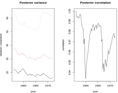
the need of multiple discounting. Also, Figure 2 plots the observation variance, covariance and correlation estimates in the time period 1956-1970. From this plot we observe that the
variability of the change in inventory time series component y2t is much larger than that of
y1t. The estimate of the observation correlation indicates the high cross-correlation between
the two series.
6
Discussion
Posterior variance
year
variance / covariance
1960 1965 1970
20
30
40
50
60
Posterior correlation
year
correlation
1960 1965 1970
0.94
0.95
0.96
0.97
0.98
0.99
[image:22.612.85.488.120.439.2]1.00
Figure 2: Posterior estimates of the observation covariance matrixV = (Vij)i,j=1,2 and
esti-mates of the correlation ρ = V12/√V11V22. In the left panel graph, shown are: estimate of
the variance V11 (solid line), estimate of the variance V12 (dashed line), and estimate of the
varianceV22 (dotted line). In the right panel graph, the solid line shows the estimate ofρ.
are indicated and, although the authors do believe that Bayes linear methods offer a great statistical tool, it is pointed out that in some problems, considered in this paper and in particular for time series data, the PSPP modelling approach can offer advantages as opposed to Bayes linear methods.
PSPP models are developed having in mind Bayesian inference for multivariate state space models when the observation covariance matrix is unknown and it is subject to estimation. This paper outlines the deficiency of the existing methods to tackle this problem and it is shown empirically that, for a class of important time series data, including local level, linear trend and seasonal components, PSPP generates much more accurate and reliable posterior estimators, which are remarkably fast and applicable to a wide range of time series data. US investment and change in inventory data are used to illustrate the capabilities of the PSPP state space models.
distributions, other than the multivariate t, the inverted multivariate t, and the Wishart distributions. In this sense a more detailed comparison of PSPP with Bayes linear methods and in particular with Bayes linear kinematics (Goldstein and Shaw, 2004), should shed more light on the performance of PSPP. It is our purpose to consider such comparisons in a future paper.
Acknowledgements
The authors are grateful to the Statistics Department at Warwick University, where this work was initiated. We are grateful to three referees for providing helpful comments.
Appendix
Proof of Theorem 1. (=⇒) By hypothesisE(X|Y) =µx+Axy(Y −µy)⇒E(X−AxyY|Y) =
µx−Axyµy = constant. Furthermore Var(X|Y) =E{(X−µx−Axy(Y−µy))(X−µx−Axy(Y−
µy))′|Y} = Σx−AxyΣyA′xy = constant ⇒ Var(X−AxyY|Y) = Var(X|Y) = constant. It
follows that X−AxyY⊥2Y.
(⇐=) The assumption X −AxyY⊥2Y implies that E(X −AxyY|Y) = µ constant ⇒
E(X|Y) = AxyY +µ, which is a linear function of Y. Given that E(X|Y) minimizes the
quadratic prior expected risk and µx +Axy(Y −µy) minimizes this risk among all linear
estimators, it follows that E(X|Y) =µx+Axy(Y −µy).
References
[1] Abraham, B. and Ledolter, A. (1983) Statistical Methods for Forecasting. Wiley, New
York.
[2] Ameen, J.R.M. and Harrison, P.J. (1984) Discount weighted estimation.Journal of
Fore-casting3, 285-296.
[3] Ameen, J.R.M. and Harrison, P.J. (1985) Normal discount Bayesian models. InBayesian
Statistics 2, J.M. Bernardo, M.H. DeGroot, D.V. Lindley, and A.F.M. Smith (Eds). North-Holland, Amsderdam, and Valencia University Press.
[4] Barbosa, E. and Harrison, P.J. (1992) Variance estimation for multivariate dynamic linear
models.Journal of Forecasting 11, 621-628.
[5] Box, G.E.P. and Tiao, G.C. (1973) Bayesian Inference in Statistical Analysis.
Addison-Wesley, Massachusetts.
[6] Dickey, J.M. (1967) Matrix-variate generalizations of the multivariate t distribution and
the inverted multivariatetdistribution.Annals of Mathematical Statistics 38, 511-518.
[7] Durbin, J. and Koopman, S.J. (2001)Time Series Analysis by State Space Methods.
Ox-ford University Press, OxOx-ford.
[8] Fahrmeir, L. (1992) Posterior mode estimation by extended Kalman filtering for
multi-variate dynamic generalized linear models.Journal of the American Statistical Association
![Figure 1: US Investment and Change in Inventory time series yt = [y1t y2t]′ with its 1-stepforecast mean ft = [f1t f2t]′](https://thumb-us.123doks.com/thumbv2/123dok_us/8079154.228534/20.612.87.487.140.441/figure-investment-change-inventory-time-series-stepforecast-mean.webp)