Learning how to act: making good decisions with machine learning

(1)

Learning how to act: making good

decisions with machine learning

Finnian Lattimore

A thesis submitted for the degree of Doctor of Philosophy

The Australian National University

November 2017

©by Finnian Rachel Lattimore, 2017

(2)

Except where acknowledged in the customary manner, the material presented in this thesis is, to the best of my knowledge, original and has not been submitted in whole or part for a degree in any university.

(3)

In vain the Sage, with retrospective eye,

Would from th’ apparent What conclude the Why, Infer the Motive from the Deed, and show,

That what we chanced, was what we meant to do.

(4)

Acknowledgements

There are many people without whose support this thesis would not have been possible. I would like to thank my supervisors Dr Cheng Soon Ong, Dr Mark Reid and Dr Tiberio Caetano, Prof. Robert Williamson for chairing my panel, my brother Tor for many in-teresting and insightful discussions on bandit problems, and my parents for helping me proofread and the many days given to care for my lovely daughters. I would also like to thank Victoria, Inger, Natalie and all the people at ANU thesis bootcamp for giving me the techniques I needed to get past the blank page and get words out. Finally I want to thank my wonderful husband for his unwavering support and willingness to take on the household chaos, and my two beautiful daughters Freya and Anouk for their patience while mummy worked on her ”tesis”.

I am also grateful for the financial support provided by an Australian Postgraduate Award and a NICTA/Data61 top up scholarship.

(5)

Abstract

This thesis is about machine learning and statistical approaches to decision making. How

can we learn from data to anticipate the consequence of, and optimally select, interventions or actions? Problems such as deciding which medication to prescribe to patients, who

should be released on bail, and how much to charge for insurance are ubiquitous, and

have far reaching impacts on our lives. There are two fundamental approaches to learning how to act: reinforcement learning, in which an agent directly intervenes in a system and

learns from the outcome, and observational causal inference, whereby we seek to infer the

outcome of an intervention from observing the system.

The goal of this thesis to connect and unify these key approaches. I introduce causal bandit

problems: a synthesis that combines causal graphical models, which were developed for

observational causal inference, with multi-armed bandit problems, which are a subset of reinforcement learning problems that are simple enough to admit formal analysis. I show

that knowledge of the causal structure allows us to transfer information learned about

the outcome of one action to predict the outcome of an alternate action, yielding a novel form of structure between bandit arms that cannot be exploited by existing algorithms. I

propose an algorithm for causal bandit problems and prove bounds on the simple regret

(6)

Introduction

1.1 Motivation

Many of the most important questions in science, commerce and our personal lives are about the outcomes of doing something. Will asking people to pay upfront at the doctors

reduce long term health expenditure? If we developed a drug to suppress particular genes,

could we cure multiple sclerosis? Would delaying teenage pregnancies improve the outcome for their children.

These are hard questions because they require more than identifying a pattern in data. Correlation is not causation. Causal inference has proven so difficult that there is barely

any consensus on even enduring questions like the returns to education or the long-term

consequences of early life events – like teenage pregnancy - despite the fact that the variables involved are susceptible to human intuition and understanding.

We now live in a world of data. Hours of our lives are spent online, where every click can

be recorded, tiny computers and sensors are cheap enough to incorporate into everything and where the US Institute of Health is considering if all infants should be genetically

sequenced at birth. Such data gives us a window into many aspects of our lives at an

unprecedented scale and detail but it is messy, complicated and often generated as a by-product of some other purpose. It does not come from the controlled world of a randomised

experiment.

The rise of big data sets and powerful computers has seen an explosion in the application

of machine learning. From health care, to entertainment and self-driving cars, machine

learning algorithms will transform many industries. It has been suggested that the im-pressive ability of statistical machine learning to detect complex patterns in huge data sets

heralds the end of theory [10] and that we may be only a short step from “The Singularity”,

where artificial intelligence exceeds our own and then grows exponentially.

However, despite the huge advances in machine learning (in particular deep learning),

(9)

them to generalise to even slightly different problems or data sets remains very challenging.

Deciding how we should act or what policies we should implement requires predictions about how a system will behave if we change it. The correlations detected by standard

machine learning algorithms do not enable us to do this, no matter how many petabytes

of data they are based on. As machine learning algorithms are incorporated into more and more of the decision making processes that shape the world we live in, it is critical

to ensure we understand the distinction between causality and prediction and that we

develop techniques for learning how to act that are as effective as those we have for pattern recognition.

1.2 What is causality?

The notion of causality has been widely debated in science and philosophy [83, 112, 124,

120, 106, 175, 75, 39] but is still viewed as poorly defined. This has led to a reluctance among applied researchers in many fields to make concrete claims about causality in their

work, leading them instead to report that variables are related, correlated or associated.

However, the magnitude, direction and even existence of an association depends on which variables are controlled for (or included in a regression). Avoiding formalising causation,

which is the real question of interest, requires the reader to determine via “common sense”

the implications of the reported associations.

There are two ways in which an association detected in a data set may be non-causal. The first is that the variables concerned may not be related at all, and the association has

arisen by chance in that data sample. Given finite data on enough variables, there is a

high probability of finding some that appear correlated even though they are completely unrelated. For example, based on data from the years 1999 to 2009, the age of Miss

America is strongly correlated with the number of murders (in the US) by steam, hot

vapours and hot objects [170]. However, this correlation is purely due to chance and does not reflect any real relationship between these variables, direct or indirect. We have no

expectation of observing this association in a new data sample. This form of spurious correlation also has serious repercussions. It lies at the heart of major problems with the

process of scientific research: researchers are incentivised to detect effects and thus to

explore many possible paths in the process of analysing data and studies that fail to find an effect are less likely to be published. Consequently, the likelihood that reported effects

have arisen by chance is underestimated, leading to the conclusion that “most published

scientific results are false” [87]. This issue is also highlighted by recent crises in replication [116]. This issue can be ameliorated by obtaining more data and by separating learning

models from evaluating their performance, for example by evaluating models on a strict

hold-out set or on the extent to which their results can be replicated.

However, a strong association, observed in multiple independent studies may still not be causal. The correlation can arise because both variables are consequences of some other,

(10)

correlated with their height, because older children are taller and can read better. However

height is not a cause of reading ability because interventions to increase a child’s height, for example by giving them growth hormones, would not be expected to improve their reading.

Similarly, extra lessons in reading will not make a child grow taller. This problem is

fundamentally different to the issue of spurious correlations arising by chance in finite data sets. Obtaining more (even infinitely many more) samples without directly intervening

in the system to manipulate the variables does not allow us to separate causation from

correlation.

The key distinction between a real, but non-causal, association and a causal relationship

is in what happens if we intervene in the system and change one of the variables. In this thesis, I take an interventionist viewpoint of causality: any model or approach designed

to predict the outcome of intervening in a system is causal. This viewpoint captures the

types of questions that motivate this thesis. How can we change the way we do things to obtain better outcomes?

Causality is often linked to explanation; understanding how and why things happen. I

view explanation in terms of compression and generalisation: the amount of information

about the world a model can capture. This creates a hierarchy in the degree to which models are explanatory, rather than a simple binary distinction. A standard predictive

model encodes all the information needed to predict some output given inputs provided

the system generating the data does not change. A high-level causal model might be able to predict the outcome of a specific intervention holding all else fixed. More detailed

causal models could predict the outcome for a wide range of combinations of interventions

conditional on a range of contexts. By considering conditional interventions within our definition of causal questions we also capture mediation: the study of pathways through

which one variable causes another [168]. Finally, a model that can distil how elements

interact into mathematical equations like Newton’s laws can be used to predict what will happen in an astounding range of settings, including many never previously observed.1

Gelman [67], Gelman and Imbens [68] make a distinction between forward causal inference, the types of “what if” questions I focus on in this thesis, and reverse causal questions,

asking why something occurs. The former aims to identify the effect of a known cause.

The latter can be viewed as identifying causes of an effect. They regard forward causal inference as well defined within the counterfactual and graphical model frameworks for

causal inference, that we describe in section 2.1. However, they state that “A reverse causal question does not in general have a well-defined answer, even in a setting where all

possible data are made available.” I view this as overly pessimistic, depending on how “all

possible data” is defined. The goal of identifying the causes of an effect can be formalised within the graphical causal model framework. Solving this problem is certainly much

more challenging than identifying the effect of a specific intervention on a given outcome,

since it requires us to test or infer the effect of interventions on many different variables. These practical difficulties may well be overwhelming, particularly in fields such as social

1

(11)

science and economics where data sets are often relatively small, systems are complex, the

variables are difficult to directly manipulate and even relatively simple ”what if” questions are hard to resolve conclusively. If some variables are fundamentally unobservable then it

may be impossible to determine all the causes of a given effect. However, this does not

mean that the problem of identifying causes of effects is ill-posed in principle. It can be viewed as a form of causal discovery: the attempt to learn the structure of the causal

relationships between variables, on which there is a rich literature, see Spirtes and Zhang

[154] for a recent review.

There has traditionally been a large gap between researchers in machine learning who focus

on prediction, using largely non-interpretable models and researchers in statistics, social

science and economics who (at least implicitly) aim to answer causal questions and tend to use highly theory-driven models. However, there is relatively little awareness, particularly

within the machine learning and data science communities, of what constitutes a causal

problem and the implications of this for the training and evaluation of models. In the next section we emphasise the subtlety that can exist in determining if a problem is causal by

examining some typical examples.

1.3 What makes a problem causal?

Machine learning is in the midst of a boom, driven by the availability of large data sets and the computation resources to process them. Machine learning techniques are being applied

to a huge range of problems, in both industry and academia. The following examples are

intended to capture the breadth of problems that machine learning algorithms are actively being applied to. Which, if any, of these problems require causal inference?

Speech recognition (for systems like Siri or Google Assistant)

Image classification

Forecasting the weather

Identifying spam emails

Automated essay marking

Predicting the risk of death in patients with pneumonia.

Predicting who will re-offend on release from prison

Customer churn modelling

Demand prediction for inventory control

Playing Go

The question is disingenuous because I have not posed the problems in sufficient detail to

(12)

any model we might build would be used: what actions would be taken in response to its

predictions.

Consider speech recognition. You say something, which causes sound waves, which are

converted to a digital signal that Siri maps to words. Whatever action Siri takes is unlikely

to change the distribution of words you use, and even less likely to change the function that maps sound waves to text (unless she sends you a DVD on elocution). A similar argument

could be made for many applications of machine translation and image classification.

In image classification we do not particularly care about building a strong model for exactly how the thing that was photographed translates to an array of pixels, provided

we can be fairly confident that the process will not change. If we develop a discriminative

model that is highly accurate at classifying cats from dogs, we do not need to understand its internal workings (assuming we have strong grounds to believe that the situations in

which we will be using our model will match those under which it was trained).

What about forecasting the weather? If you are using a short term forecast to decide whether to pack an umbrella, causality can be ignored. Your decision will not affect if it

actually rains. However, longer term climate forecasts might (theoretically) lead to action

on emissions which would then change the weather system. For this we need a (causal) model that allows us to predict the outcome under various different interventions.

Identifying spam and automated essay marking both involve processing text to determine

an underlying (complex) attribute such as its topic or quality. In both cases, there is inherent competition between the algorithm and the people generating the text. As a

result, decisions made by the algorithm are likely to change the relationship between the

features it relies on and the true label. Spammers and students will modify their writing in order to optimise their results. A standard supervised learning approach can only work

if the resulting change in the mapping from features to label is sufficiently gradual. There

are two key ways of ensuring this. The first is to limit people’s ability to observe (and thus react to) decisions made by the algorithm. The second is to use a model in which the

features are related to the outcome such that they cannot be manipulated independently

so that people’s attempts to modify features in order to obtain a desired prediction also alter the true label.

This example also highlights a connection between causal models and transparency in

ma-chine learning. If we are using a non-causal model to make decisions affecting people, there will be a trade-off between the performance and transparency of the model; not because

the requirement for transparency restricts us to simple models, but because revealing how

the model works allows people to change their behaviour to game it.

What about predicting the risk of death in patients with pneumonia? Suppose the goal is

to build a model to decide who should be treated in hospital and who can be sent home

with antibiotics. If we assume that in hospital treatment is more effective for serious cases, this appears to be straightforward prediction. It is not. Depending on how the

(13)

the model, the relationship between those features and the outcome may change if the

model is used to make admission decisions. Caruana et al. [40] found exactly this effect in a real data set. The model learned that people suffering asthma were less likely to die

from pneumonia. This was because doctors treated such patients very aggressively, thus

actually lowering their risk. The issue is not with the model; it performed very well at the task for which it was trained, which is to predict who would be likely to die under the

original admission and treatment protocols. However, using it to decide how to change

these protocols could kill. The actual question of interest in this case is what happens to patients with characteristics X if they are assigned treatment according to decision rule

(or policy)π(X).

Predicting recidivism among paroled prisoners or customer churn also fit within the class of problems where the goal is to identify a group for which a problem will occur in order to

target treatment (additional support and monitoring for people on parole, loyalty rewards to improve customer retention, hospitalisation for the severely ill). Predictive models

can be applied to such problems where the most effective treatment is known for a given

target group, and where deciding who to treat on the basis of the model predictions will not change the relationship between the features and outcome.

Demand prediction seems like a relatively straightforward prediction problem. Models use

features such as location, pricing, marketing, time of year and weather, to forecast the demand for a product. It seems unlikely that using the model to ensure stock is available

will itself change demand. However, depending on the way demand is measured, there is

a potential data censoring issue. If demand is modelled by the number of sales, then if a product is out of stock demand will appear to be zero. Changing availability does then

change demand.

Playing Go (and other games) is a case with some subtleties. At every turn, the AI

agent has a number of actions available. The state of the board following each action

is deterministic and given by the rules of the game. The agent can apply supervised machine learning, based on millions of previous games, to estimate the probability that

each of these reachable board states will lead to a win.2 Supervised learning can also be applied to learn a policy P (a|s), the probability of a player selecting action a, given board state s. This allows the agent to estimate the likelihood of winning from a given

starting state by simulating many times the remainder of the game, drawing actions from

P (a|s) for both players. Google’s Alpha Go, which in May 2017 beat the then strongest human player [114], incorporates a combination of these approaches [148]. The supervised

learning was enhanced by having the agent play (variants) of itself many times, so that its

estimates of value for each board state and of the likelihood an opponent will play a given move are based on a combination of replicating the way humans play and on the moves

that led to a win when playing itself.

2

(14)

The problem of playing go is causal from the interventionalist perspective. The agent

wishes to learn the probability of a win given an action they take. However, there are some special characteristics of the go problem that make it amenable to a primarily supervised

learning approach. The actions the agent has to explore are the same ones as human

players explored to generate the training data, and both have the same objective - to win the game. In addition, the state of the board encapsulates all the information relevant to

selecting a move. These factors make it reasonable to conclude that selecting moves with

an algorithm will not change the value of a board state or the probability of given move by the opponent by a sufficiently large margin to invalidate the training data.

Having considered these examples we can now identify some general aspects of problems

that require causal (as opposed to purely predictive) inference. A predictive model may be sufficient if, given the variable(s) being predicted, it is clear which action is optimal and if

selecting actions on the basis of the model does not change the mapping from features to

outcomes. The second requirement is particularly difficult to satisfy when an algorithm is making important decisions affecting individual people. Think about problems like credit

scoring and parole decisions. There are strong ethical grounds for demanding transparency,

but if the goals of society and the individuals are not perfectly aligned and there is any possibility that people can manipulate features independently of the outcome, there will

be a conflict between model accuracy and transparency. It is rare to build a model without

any intent to make some kind of decision based on its results. Thus, I argue we should assume a causal model is required until we can justify otherwise.

1.4 Observe or intervene: two very different approaches to

causal problems

As we have shown, problems involving causality are ubiquitous in many fields. As a result,

techniques for addressing them have developed in parallel within many disciplines, includ-ing statistics, economics, social science, epidemiology and machine learninclud-ing. Although

the focus and terminology can differ substantially between fields, these techniques all

ad-dress the underlying goal of estimating the effect of, or optimally selecting, interventions in some system. Methods for learning about interventions can be usefully categorised

into two broad approaches, based on whether or not the algorithm has control over what

actions are taken, reinforcement learning and observational causal inference.

In reinforcement learning, under which we include traditional randomised experiments, we

learn the outcome of actions by taking them. We take the role of an agent, capable of

inter-vening in the system, and aim to develop algorithms that allow the agent to select actions optimally with respect to some goal. A particular strand of research within reinforcement

learning are multi-armed bandit problems. They describe settings in which there is a set

of available actions, the agent repeatedly decides which to select and then observes the outcome of the chosen action. They capture problems, such as a doctor deciding which

(15)

display to a user, where the agent faces the same set of choices repeatedly and is able to

assess the value of the outcome they observe.

The approach of learning the outcome of an action by taking it plays a key role in

ad-vancing our knowledge of the world. However, we frequently have access to large bodies

of data that have been collected from a system in which we did not have any control over what actions were taken, or perfect knowledge of the basis on which those actions were

chosen. Estimating the effect of an action from such observational data sets is the problem

addressed by observational causal inference. Observational causal inference can be viewed as a form of transfer learning. The goal is to leverage data obtained from one system, the

system we have observed, to estimate key characteristics of another, the system after we

select an action via some policy that may differ from the process driving which actions occur in the original system. This is impossible without some assumptions about how the

original system and the system after intervention are related to one-another. The key to

observational inference is to model how actions change the state of the world in such a way that we can map information collected in one setting to another.

Another difference between the reinforcement learning and observational causal inference

communities is the focus on i.i.d vs non i.i.d data. Because reinforcement learning covers settings where an agent is explicitly intervening in and thus changing the system,

algo-rithms are typically developed with non-i.i.d data in mind. In contrast much of the work in observational causal inference is applied to cross-sectional data under the assumption

that the system is in some form of equilibrium such that the data can be treated as i.i.d.

However, this difference is not fundamental: Randomised experiments can be viewed as a special case of reinforcement learning with i.i.d data and there is a substantial body of

work on causal inference from time-series that leverages the assumption that the future

does not cause the past [70]. The problem of off-policy evaluation [100] on data gener-ated by a non-stationary policy can be viewed as an example of an observational causal

inference problem over non-i.i.d data.

Both multi-armed bandits and observational causal inference can be seen as extensions to the concept of randomised controlled trials. Bandit algorithms deal with the

sequen-tial nature of the decision making process, and causal inference with problems where

randomisation is not feasible, affordable or ethical. The similarities between the prob-lems addressed by these techniques raise the question of whether there are probprob-lems best

addressed by a combination of these approaches, and if so, how they can be combined.

1.5 This thesis and its contributions

I view causal problems as one of the greatest current challenges for machine learning.

They incorporate a large set of problems of huge practical significance, that require us to go beyond pattern recognition, but are well short of general artificial intelligence. For

(16)

learning to be effectively applied in many areas of medicine, economics, social sciences and

industry, we need to understand how to leverage our improved approaches to prediction to tackle causal problems.

Contributions The goal of this thesis is to connect and unify the key approaches to solving causal problems from both the observational and interventional viewpoints. My

major contribution unifies the causal graphical model approach for inference in observa-tional settings with the sequential experimental approach encapsulated by multi-armed

bandits. This synthesis allows us to represent knowledge of how variables are related to one-another in a very natural way and induces an interesting and novel form of structure

between the different actions modelled in the bandit problem. I develop a new algorithm

that can exploit this structure as a first step towards a unified approach to decision making under uncertainty.

I also make a number of additional connective contributions that are not encompassed by

my work on causal bandit problems. I demonstrate the role of a formal causal framework

within Bayesian approaches to inference and show how assigning a prior based on human causal intuition without considering the causal structure of the problem can introduce bias.

I highlight the connections between approaches to off-policy evaluation in bandit problems,

causal effect estimation from observational data, and covariate shift. Finally, I clarify the implicit causal structure underlying various bandit settings and the counterfactual nature

of regret - the measure by which bandit algorithms are assessed.

Thesis overview This thesis is divided into three key chapters: learning from obser-vational data, learning from interventional data and unifying the approaches. Chapter 2

covers learning to act from observational data, where the goal is to learn the outcome of

an external intervention in a system from data obtained by observing it without control over which actions are selected. In§2.1, I describe the key existing frameworks for causal

inference from observational data, discuss how they relate to one-another and introduce

the notation required to describe causal problems. Section §2.2 describes the key tools these frameworks provide that enable us to answer causal questions, in particular, the

do-calculus (§2.2.1.2) and, in sections §2.2.2 and §2.2.3, discusses how we define causal

effects, the traditional approaches to estimation and how they relate to covariate shift and off-policy evaluation. Section §2.3 highlights the role graphical causal models can play in

Bayesian inference.

Chapter 3 deals with the interventionalist viewpoint, including traditional randomised

ex-periments (§3.1) and multi-armed bandit problems. In §3.2, I describe the key problems and results within the bandit literature, including stochastic bandits (§3.2.1), pure

ex-ploration problems (§3.2.2), adversarial bandits (§3.2.3) and contextual bandits (§3.2.4).

I clarify the causal structure of (stochastic) contextual bandit problems in §3.2.4.1. In

(17)

in§3.3 I discuss the counterfactual nature of bandit regret.

In chapter 4, I introduce causal bandit problems that unify causal graphical models and

multi-armed bandit problems. Bandit arms are related to interventions in a causal graph-ical model in a very natural way: each multi-armed bandit arm (or action) corresponds to

a particular assignment of values to variables within the causal graphical model. I show

how the causal bandit framework can be used to describe a number of existing problems that lie in the intersection between the observational and interventional approaches to

causality and demonstrate when causal bandit problems reduce to different existing

ban-dit settings depending what information is observable and when. I focus on analysing the simple regret which arises in problems where exploration and exploitation are seperated

into different phases and the goal is to identify an action that is close to optimal with high probability within the exploration period. I demonstrate that knowlege of the causal

structure reduces the effective number of arms to explore, resulting in faster exploration.

Although I have analysed only the simple regret, causal structure could also be leveraged to improve cummulative regret.

In §4.2, I focus on causal bandit problems for which the values of variables in the causal

graph are observed after an action is selected. I demonstrate that this leads to a novel

form of structure between the bandit arms that cannot be exploited by existing bandit algorithms.

In §4.2.1, I describe and develop an algorithm for a special case of the causal bandit

problem, which I refer to as theparallel bandit problem. I demonstrate via upper and lower bounds on the regret that the algorithm is close to optimal for these problems and that

the introduction of the causal structure leads to substantially faster learning. In §4.2.2, I

develop and prove regret bounds for an algorithm that can be applied to arbitrary causal graphs, albeit with stronger assumptions on what must be known a priori, and introduce a

measure that captures the underlying difficulty of causal bandit problems, which depends

on the causal graph and can be viewed as an “effective number of arms”. I also show how this measure can be used to quantify the value of optimised interventional data over purely

observational data. Section 4.2.3 provides experiments demonstrating the performance of

(18)

Chapter 2

Learning from observational data

The goal of causal inference is to learn the effect of taking an action. We can do this directly via experimental approaches, however any given agent only has a limited capacity

to manipulate the world. We are generating and storing data on almost every aspect

of our lives at an unprecedented rate. As we incorporate sensors and robotics into our cities, homes, cars, everyday products and even our bodies, the breadth and scale of this

data will only increase. However, only a tiny fraction of this data will be generated in a

controlled way with the specific goal of answering a single question. An agent that can only learn from data when it had explicit control (or perfect knowledge of) the process

by which that data was generated will be severely limited. This makes it critical that

we develop effective methods that enable us to predict the outcome of an intervention in some system by observing, rather than acting on it. This is the problem of observational

causal inference. The key feature that distinguishes observational from interventional data

is that the learning agent does not control the action about which they are trying to learn.

2.1 Causal models

Observational causal inference aims to infer the outcome of an intervention in some system

from data obtained by observing (but not intervening on) it. As previously mentioned, this

is a form of transfer learning; we need to infer properties of the system post-intervention from observations of the system pre-intervention. Mapping properties from one system

to another requires some assumptions about how these two systems are related, or in

other words, a way of describing actions and how we anticipate a system will respond to them. Three key approaches have emerged: counterfactuals, structural equation models

and causal Bayesian networks.

Counterfactuals [138] were developed from the starting point of generalising from

ran-domised trials to less controlled settings. They describe causal effects in terms of differ-ences between counterfactual variables, what would happen if we took one action versus

(19)

naturally in human languages and are prevalent in everyday conversations; “if I had worked

harder I would have got better grades” and “she would have been much sicker if she hadn’t taken antibiotics”. Structural equation models have been developed and applied primarily

within economics and related disciplines. They can be seen as an attempt to capture key

aspects of the people’s behaviour with mathematics. Questions around designing policies or interventions play a central role in economics. Thus they have transformed

simulta-neous equations into a powerful framework and associated set of methods for estimating

causal effects. The is also a rich strand of work on using the assumptions that can be encoded in structural equation models, also known as functional causal models to discover

the structure and direction of causal relationships - see for example [113, 125]. Causal

Bayesian networks [120] are a more recent development and arise from the addition of a fundamental assumption about the meaning of a link to Bayesian networks. They

in-herit and leverage the way Bayesian networks encode conditional independencies between

variables to localise the impact of an intervention in a system in a way that allows for-malisation of the conditions under which causal effects can be inferred from observational

data.

An understanding of causal Bayesian networks and their properties (in particular the do

calculus, see section 2.2.1.2) is sufficient to appreciate my main technical contributions in chapter 4, as well as the importance of formal causal reasoning in Bayesian inference that

I highlight in section 2.3. However, the literature on causal inference techniques remains

split between the different frameworks. Much of the recent work on estimating causal effects within machine learning, as well as widely used methodologies such as propensity

scoring, are described using the counterfactual framework. Methods developed within

economics, in particular instrumental variable based approaches, or those requiring para-metric or functional assumptions, are often based around structural equation models. This

makes it worthwhile for researchers interested in causality to develop an understanding of

all these viewpoints.

In the next sections, we describe causal Bayesian networks, counterfactuals and structural equation models: the problems they allow us to solve, the assumptions they rely on and

how they differ. By describing all three frameworks, how they relate to one-another, and

when they can be viewed as equivalent, we will make it easier for researchers familiar with one framework to understand the others and to transfer ideas and techniques between

them. However, sections 2.1.3 (Structural Equation models), and 2.1.4 (Unifying the

models) are not crucial to understanding my technical contributions and may be safely skipped. In order to demonstrate the notation and formalisms each framework provides,

we will use them to describe the following simple examples.

Example 1. Suppose a pharmaceutical company wants to assess the effectiveness of a new drug on recovery from a given illness. This is typically tested by taking a large group

of representative patients and randomly assigning half of them to a treatment group (who receive the drug) and the other half to a control group (who receive a placebo). The

(20)

the outcomes for the two groups (in this case, simplified to only two outcomes - recovery

or non-recovery). We will use the variable X (1 = drug, 0 = placebo) to represent the treatment each person receives and Y (1 = recover, 0 = not recover) to describe the

outcome.

Example 2. Suppose we want to estimate the impact on high school graduation rates of compulsory preschool for all four year olds. We have a large cross-sectional data set on a

group of twenty year olds that records if they attended preschool, if they graduated high school and their parents socio-economic status (SES). We will let X ∈ {0,1} indicate if

an individual attended preschool, Y ∈ {0,1} indicate if they graduated high school and

Z ∈ {0,1} represent if they are from a low or high SES background respectively.1

2.1.1 Causal Bayesian networks

Causal Bayesian networks are an extension of Bayesian networks. A Bayesian network is

a graphical way of representing how a distribution factorises. Any joint probability dis-tribution can be factorised into a product of conditional probabilities. There are multiple

valid factorisations, corresponding to permutations of variable ordering.

P(X1, X2, X3, ...) =P(X1)P(X2|X1)P(X3|X1, X2)... (2.1)

We can represent this graphically by drawing a network with a node for each variable

and adding links from the variables on the right hand side to the variable on the left for each conditional probability distribution, see figure 2.1. If the factorisation simplifies due

to conditional independencies between variables, this is reflected by missing edges in the

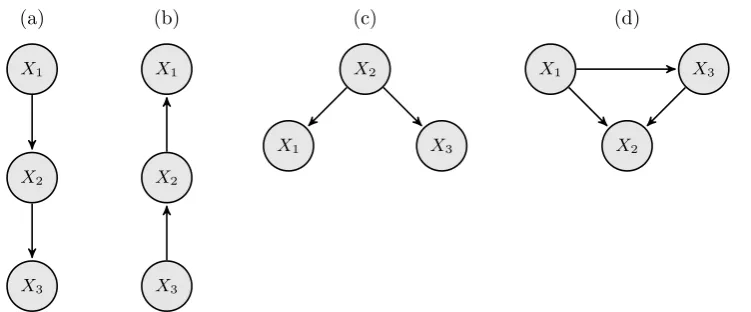
corresponding network. There are multiple valid Bayesian network representations for any probability distribution over more than one variable, see figure 2.2 for an example.

X1

X2 X3

Figure 2.1: A general Bayesian network for the joint distribution over three variables. This network does not encode any conditional independencies between its variables and can thus represent any distribution over three variables.

The statement that a given graph G is a Bayesian network for a distribution P tells us

that the distribution can be factorised over the nodes and edges in the graph. There can be no missing edges inGthat do not correspond to conditional independencies inP, (the

converse is not true: G can have extra edges). If we let parentsXi represent the set of

1

(21)

(a)

X1

X2

X3

(b)

X1

X2

X3

(c)

X2

X1 X3

(d)

X2

[image:21.595.145.521.53.209.2]

X1 X3

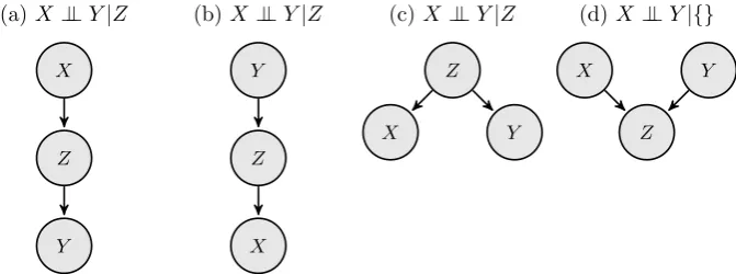
Figure 2.2: Some valid Bayesian networks for a distribution P over (X1, X2, X3) in which X3 is conditionally independent of X1 given X2, denoted X3 ⊥⊥ X1|X2. Graphs (a), (b)

and (c) are all a perfect map for P as the graphical structure implies exactly the same set of independencies exhibited by the distribution. Graph (d), like figure 2.1 does not imply any conditional independencies, and is thus a valid (but not very useful) Bayesian network representation for any distribution over three variables.

variables that are parents of the variableXi inGthen we can write the joint distribution

as;

P (X1, ..., XN) =

Y

i=1...N

P (Xi|parentsXi) (2.2)

A causal Bayesian network is a Bayesian network in which a linkXi→Xj, by definition,

implies Xi directly2 causes Xj. This means an intervention to change the value of Xi

can be expected to affect Xj, but interventions onXj will not affect Xi. We need some

notation to describe interventions and represent distributions over variables in the network after an intervention. In this thesis, I use the do operator introduced by Pearl [120].

Definition 3. The do-notation

do(X=x) denotes an intervention that sets the random variable(s)X tox.

P (Y|do(X)) is the distribution ofY conditional on anintervention that setsX. This notation is somewhat overloaded. It may be used to represent a probability distri-bution/mass function or a family of distribution functions depending on whether

the variables are discrete or continuous and whether or not we are treating them as

fixed. For example, it could represent

– the probability P (Y = 1|do(X=x)) as a function ofx,

– the probability mass function for a discreteY : P (Y|do(X=x)),

– the probability density function for a continuousY : fY(y|do(X=x)),

2

(22)

– a family of density/mass function for Y parameterised by x.

Where the distinction is important and not clear from context we will use one of the

more specific forms above.

Theorem 4 (Truncated product formula [120]). If G is a causal network for a distri-bution P defined over variables X1...XN, then we can calculate the distribution after an

intervention where we set Z ⊂X to z, denoted do(Z=z) by dropping the terms for each of the variables in Z from the factorisation given by the network. Let PaXi denote the

parents of the variable Xi in G.

P (X1...XN|do(Z=z)) =1{Z =z}

Y

Xi∈/Z

P (Xi| PaXi) (2.3)

Theorem 4 does not hold for standard Bayesian networks because there are multiple valid

networks for the same distribution. The truncated product formula will give different

results depending on the selected network. The result is possible with causal Bayesian networks because it follows directly from the assumption that the direction of the link

indicates causality. In fact, from the interventionist viewpoint of causality, the truncated

product formula defines what it means for a link to be causal.

Returning to example 1, and phrasing our query in terms of interventions; what would

the distribution of outcomes look like if everyone was treated P (Y|do(X= 1)), relative

to if no one was treated P (Y|do(X = 0))? The treatment X is a potential cause of Y, along with other unobserved variables, such as the age, gender and the disease subtype

of the patient. Since X is assigned via deliberate randomisation, it cannot be affected

by any latent variables. The causal Bayesian network for this scenario is shown in figure 2.3. This network represents the (causal) factorisation P (X, Y) = P (X) P (Y|X), so from

equation (2.3), P (Y|do(X)) = P (Y|X). In this example, the interventional distribution

is equivalent to the observational one.

X (Treatment) Y (Outcome)

Figure 2.3: Causal Bayesian network for example 1

In example 2 we are interested in P (Y|do(X= 1)), the expected high-school graduation

rate if we introduce universal preschool. We could compare it to outlawing preschool

P (Y|do(X= 0)) or the current status quo P (Y). It seems reasonable to assume that preschool attendance affects the likelihood of high school graduation3 and that parental socio-economic status would affect both the likelihood of preschool attendance and high

school graduation. If we assume that socio-economic status is the only such variable (nothing else affects both attendanceand graduation), we can represent this problem with

the causal Bayesian network in figure 2.4. In this case, the interventional distribution is not

3

(23)

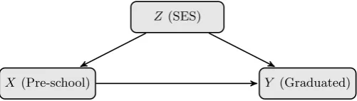
Z (SES)

[image:23.595.201.452.56.127.2]

X (Pre-school) Y (Graduated) Figure 2.4: Causal Bayesian network for example 2

equivalent to the observational one. If parents with high socio-economic status are more

likely to send their children to preschool and these children are more likely to graduate high school regardless, comparing the graduation rates of those who attended preschool

with those who did not will overstate the benefit of preschool. To obtain the interventional

distribution we have to estimate the impact of preschool on high school graduation for each socio-economic level separately and then weight the results by the proportion of the

population in that group,

P (Y|do(X= 1)) = X

z∈Z

P (Y|X = 1, Z) P (Z) (2.4)

We have seen from these two examples that the expression to estimate the causal effect of an intervention depends on the structure of the causal graph. There is a very powerful

and general set of rules that specifies how we can transform observational distributions

into interventional ones for a given graph structure. These rules are referred to as the Do-calculus [120]. We discuss them further in section 2.2.1.2.

A causal Bayesian network represents much more information than a Bayesian network

with identical structure. A causal network encodes all possible interventions that could be specified with the do-notation. For example, if the network in figure 2.4 were an ordinary

Bayesian network and all the variables were binary, the associated distribution could

be described by seven parameters. The equivalent causal Bayesian network additionally represents the post-interventional distributions for six possible single variable interventions

and twelve possible two variable interventions. Encoding all this information without the

assumptions implicit in the causal Bayesian network would require an additional thirty parameters.4

Causal Bayesian networks are Bayesian networks, so results that apply to Bayesian

net-works carry directly across: the local Markov property states that variables are inde-pendent of their non-effects given their direct causes. The global Markov property and

d-separation also hold in causal networks. D-separation, which characterises which

con-ditional independencies must hold in any distribution that can be represented by a given Bayesian networkG, is key to many important results and algorithms for causal inference.

4

(24)

We include a brief review of D-separation in section 2.2.1.1.

2.1.1.1 Limitations of causal Bayesian networks

A number of criticisms have been levelled at this approach to modelling causality. One

is that the definition of an intervention only in terms of setting the value of one or more variables is too precise and that any real world intervention will affect many variables in

complex and non-deterministic ways [132, 39]. However, by augmenting the causal graph

with additional variables that model how interventions may take effect, the deterministic do operator can model more complex interventions. For example, in the drug treatment

case, we assumed that all subjects complied, taking the treatment or placebo as assigned by the experimenter. But, what if some people failed to take the prescribed treatment? We

can model this within the framework of deterministic interventions by adding a node

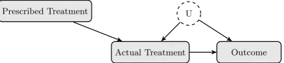
rep-resenting what they were prescribed (the intervention) which probabilistically influences the treatment they actually receive (figure 2.5). Note that the fact that we no longer

di-rectly assign the treatment opens the possibility that an unobserved latent variable could

affect both the actual treatment taken and the outcome.

Prescribed Treatment

[image:24.595.127.416.401.465.2]

Actual Treatment Outcome U

Figure 2.5: Randomised treatment with imperfect compliance

Another key issue with causal Bayesian networks is that they cannot handle cyclic de-pendencies between variables. Such feedback loops are common in real-life systems, for

example the relationship between supply and demand in economics or predator and prey

in ecology. We might regard the underlying causal mechanisms in these examples to be acyclic; the number of predators at one time influences the number of prey in the next

pe-riod and so on. However, if our measurements of these variables must be aggregated over

time periods that are longer than the scale at which these interactions occur, the result is a cyclical dependency. Even were we able to measure on shorter timescales, there might

then not be sufficient data on each variable for inference. Such problems have mostly been

studied within the dynamical systems literature, typically focusing on understanding the stationary or equilibrium state of the system and making very specific assumptions about

functional form in order to make problems tractable. Poole and Crowley [127] compare the

equilibrium approach to reasoning about cyclic problems with structural equation models, which we discuss in section 2.1.3 and that can be seen as Bayesian causal networks with

(25)

2.1.2 Counterfactuals

The Neyman-Rubin model [138, 139, 136, 140, 141] defines causality in terms of potential

outcomes, or counterfactuals. Counterfactuals are statements about imagined or alternate

realities, are prevalent in everyday language and may play a role in the development of causal reasoning in humans [173]. Causal effects are differences in counterfactual variables:

what the difference is between what would have happened if we did one thing versus what would have happened if we did something else.

In example 1, the causal effect of the drug relative to placebo for personiis the difference

between what would have happened if they were given the drug, denoted yi1 versus what

would have happened if they got the placebo, yi0. The fundamental problem of causal

inference is that we can only observe one of these two outcomes, since a given person can

only be treated or not treated. The problem can be resolved if, instead of people, there are units that can be assumed to be identical or that will revert exactly to their initial state

some time after treatment. This type of assumption often holds to a good approximation

in the natural sciences and explains why researchers in these fields are less concerned with causal theory.

Putting aside any estimates of individual causal effects, it is possible to learn something

about the distributions under treatment or placebo. LetY1 be a random variable repre-senting the potential outcome if treated. The distribution of Y1 is the distribution of Y

if everyone was treated. Similarly Y0 represents the potential outcome for the placebo. The difference between the probability of recovery, across the population, if everyone was treated and the probability of recovery if everyone received the placebo is P Y1

−P Y0

.

We can estimate (from an experimental or observational study):

P (Y = 1|X= 1), the probability that those who took the treatment will recover

P (Y = 1|X= 0), the probability that those who were not treated will recover

Now, for those who took the treatment, the outcome had they taken the treatmentY1 is the same as the observed outcome. For those who did not take the treatment, the observed outcome is the same as the outcomehadthey not taken the treatment. Equivalently stated:

P Y0|X = 0

= P (Y|X = 0)

P Y1|X = 1= P (Y|X = 1)

If we assumeX⊥⊥Y0 and X⊥⊥Y1:

P Y1

= P Y1|X= 1

= P (Y|X= 1)

(26)

This implies the counterfactual distributions are equivalent to the corresponding

condi-tional distributions and, for a binary outcome Y, the causal effect is,

P Y1−P Y0= P (Y|X= 1)−P (Y|X= 0)

The assumptions X⊥⊥Y1 and X⊥⊥Y0 are referred to as ignorability assumptions [136]. They state that the treatment each person receives is independent of whether they would

recover if treated and if they would recover if not treated. This is justified in example 1 due to the randomisation of treatment assignment. In general the treatment assignment will

not be independent of the potential outcomes. In example 2, the children from wealthy

families could be more likely to attend preschool but also more likely to do better in school regardless, i.e X 6⊥⊥Y0 _and _X _6⊥_⊥_Y1_{. A more general form of the ignorability assumption}

is to identify a set of variables Z such thatX⊥⊥Y1|Z and X⊥⊥Y0|Z.

Theorem 5 (Ignorability [136, 120]). If X⊥⊥Y1_|_Z _and _X _⊥_⊥_Y0_|_Z_,

P Y1=X

z∈Z

P (Y|X= 1, Z) P (Z) (2.5)

P Y0

=X

z∈Z

P (Y|X= 0, Z) P (Z) (2.6)

Assuming that within each socio-economic status level, attendance at preschool is

indepen-dent of the likelihood of graduating high-school had a person attended, then the average

rate of high-school graduation given a universal preschool program can be computed from equation 2.5. Note, that this agrees with the weighted adjustment formula in equation

2.4.

Another assumption introduced within the Neyman-Rubin causal framework is the

Sta-ble Unit Treatment Value Assumption (SUTVA) [139]. This is the assumption that the

potential outcome for one individual (or unit) does not depend on the treatment assigned to another individual. As an example of a SUTVA violation, suppose disadvantaged four

year olds were randomly assigned to attend preschool. The subsequent school results of

children in the control group, who did not attend, could be boosted by the improved be-haviour of those who did and who now share the classroom with them. SUTVA violations

would manifest as a form of model misspecification in causal Bayesian networks.

There are objections to counterfactuals arising from the way they describe alternate uni-verses that were never realised. In particular, statements involving joint distributions over

counterfactual variables may not be able to be validated empirically Dawid [46]. One way

of looking at counterfactuals is as a natural language short hand for describing highly specific interventions like those denoted by the do-notation. Rather than talking about

(27)

system constant we just say what would the distribution of Y be had X been x. This

is certainly convenient, if rather imprecise. However, the ease with which we can make statements with counterfactuals that cannot be tested with empirical data warrants

care-ful attention. It is important to be clear what assumptions are being made and whether

or not they could be validated (at least in theory).

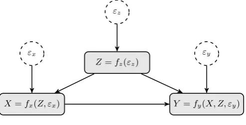
2.1.3 Structural Equation models

Structural equation models (SEMs) describe a deterministic world, where some underlying

mechanism or function determines the output of any process for a given input. The

mechanism (but not the output) is assumed to be independent of what is fed into it. Uncertainties are not inherent but arise from unmeasured variables. Linear structural

equation models have a long history for causal estimation [177, 71]. More recently, they

have been formalised, generalised to the non-linear setting and connected to developments in graphical models to provide a powerful causal framework [120].

Mathematically, each variable is a deterministic function of its direct causes and a noise

term that captures unmeasured variables. The noise terms are required to be mutually independent. If there is the possibility that an unmeasured variable influences more than

one variable of interest in a study, it must be modelled explicitly as a latent variable.

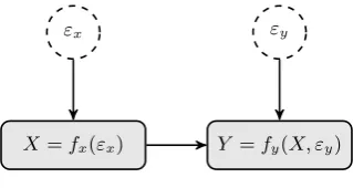
Structural equation models can be represented visually as a network. Each variable is a node and arrows are drawn from causes to their effects. Figure 2.6 illustrates the SEM for

example 1.

X =fx(εx) Y =fy(X, εy)

εy

[image:27.595.246.406.448.533.2]

εx

Figure 2.6: SEM for example 1

This model encodes the assumption that the outcomeyi for an individualiis caused solely

by the treatment xi they receive and other factorsεyi that are independent of X. This is

justifiable on the grounds that X is random. The outcome of a coin flip for each patient

should not be related to any of their characteristics (hidden or otherwise). Note that the causal graph in figure 2.6 is identical to that of the Bayesian network for the same problem

(figure 2.3). The latent variables εx and εy are not explicitly drawn in figure 2.3 as they

are captured by the probabilistic nature of the nodes in a Bayesian network.

Taking theaction X = 1 corresponds to replacing the equation X =fx(εx) withX = 1.

The functionfyand distribution overεydoes not change. This results in the interventional

distribution, 5

5

(28)

P (Y =y|do(X= 1)) =X

εy

P (εy)1{fy(1, εy) =y} (2.7)

The observational distribution ofY given X is,

P (Y =y|X = 1) =X

εx X

εy

P (εx|X= 1) P (εy|εx)1{fy(1, εy) =y} (2.8)

=X

εy

P (εy)1{fy(1, εy) =y}, asεx⊥⊥εy (2.9)

The interventional distribution is the same as the observational one. The same argument

applies to the intervention do(X = 0), and so the causal effect is simply the difference in observed outcomes as found via the causal Bayesian network and counterfactual

ap-proaches.

The SEM for example 2 is shown in figure 2.7. Intervening to send all children to preschool

replaces the equation X = fx(Z, εx) with X = 1, leaving all the other functions and

distributions in the model unchanged.

P (Y =y|do(X = 1)) =X

z

X

εy

P (z) P (εy)1{fy(1, z, εy) =y} (2.10)

=X

z

P (z)X

εy

P (εy)1{fy(1, z, εy) =y}

| {z }

P(Y=y|X=1,Z=z)

(2.11)

Equation 2.11 corresponds to equations 2.4 and 2.5. It is not equivalent to the

observa-tional distribution given by:

P (Y =y|X = 1) =X

z

X

εy

P (z|X = 1) P (εy)1{fy(1, z, εy) =y} (2.12)

Structural equation models are generally applied with strong constraints on the functional

form of the relationship between the variables and noise, which is typically assumed to

be additive, Xi = fi(·) +εi. A structural equation model with N variables resembles

a set of N simultaneous equations, with each variable playing the role of the dependent

(left hand side) variable in one equation. However a SEM is, by definition, more than

a set of simultaneous equations. By declaring it to be structural, we are saying that it representscausal assumptions about the relationships between variables. When visualised

(29)

X=fx(Z, εx)

Z=fz(εz)

εz

Y =fy(X, Z, εy)

εy

[image:29.595.204.451.57.183.2]

εx

Figure 2.7: SEM for example 2

that one does not cause the other. The similarity between the notation used to describe

and analyse structural equation models and simultaneous equations, combined with a reluctance to make explicit statements about causality, has led to some confusion in the

interpretation of SEMs [74, 120].

Granger causality A discussion of approaches to (observational) causal inference would not be complete without a mention of Granger causality, [70]. The fundamental idea

behind Granger causality is to leverage the assumption that the future does not cause the past to test the existence and direction of a causal link between two time series.

The basic approach is to test, for a pair of time series variables X and Y, if Yt ⊥⊥

(X1, ..., Xt−1)|(Y1, ..., Yt−1) - that is if the history ofXhelps to predictY given the history

of Y. The original formulation considered only pairs of variables and linear causal

rela-tionships but recent work has generalised the key idea to multiple variables and non-linear

relationships. Unlike the previous models we have discussed, Granger causality does not provide us with a means to specify our assumptions about the causal structure between

variables. Rather it aims to infer the causal structure of a structural equation model from

observational data - subject to some assumptions. I would categorise Granger causality as method for causal discovery in time series data, see the discussion of causal discovery

versus causal effect estimation in section 2.2.

2.1.4 Comparing and unifying the models

Remarkably for models developed relatively independently in fields with very different

approaches and problems, causal Bayesian networks, counterfactuals and structural equa-tion models can be nicely unified for intervenequa-tional queries (those that can be expressed

with the do-notation) [120]. These queries, and the assumptions required to answer them,

can be mapped between the frameworks in a straightforward way, allowing techniques de-veloped within one framework to be immediately applied within another. If the network

for a structural equation model is acyclic, that is if starting from any node and following

edges in the direction of the arrows you cannot return to the starting point, then it implies a recursive factorisation of the joint distribution over its variables. In other words, the

(30)

networks also apply to acyclic structural equation models. Taking an action that sets a

variable to a specific value equates to replacing the equation for that variable with a con-stant. This corresponds to dropping a term in the factorisation and the truncated product

formula (equation 2.3). Thus, the interventional query P(Y|do(X)) is identical in these

two frameworks. We can also connect this to counterfactuals via:

P Y0≡P(Y|do(X = 0)) P Y1≡P(Y|do(X = 1))

(2.13)

The assumptionεX ⊥⊥εY, stated for our structural equation model, impliesX⊥⊥(Y0, Y1)

in the language of counterfactuals. When discussing the counterfactual model, we made

the slightly weaker assumption:

X⊥⊥Y0 and X⊥⊥Y1 (2.14)

It is possible to relax the independence of errors assumption for SEMs to correspond

exactly with the form of equation (2.14) without losing any of the power provided by

d-separation and graphical identification rules [131]. The correspondence between the models for interventional queries (those that can be phrased using the do-notation) makes

it straightforward to combine key results and algorithms developed within any of these

frameworks. For example, you can draw a causal graphical network to determine if a problem is identifiable and which variables should be adjusted for to obtain an unbiased

causal estimate. Then use propensity scores [136] to estimate the effect. If non-parametric

assumptions are insufficient for identification or lead to overly large uncertainties, you can specify additional assumptions by phrasing your model in terms of structural equations.

The frameworks do differ when it comes to causal queries that involve joint or nested

counterfactuals and cannot be expressed with the do-notation. These types of queries arise in the study of mediation [123, 84, 169] and in legal decisions, particularly on issues such

as discrimination [120, Ch. 4, Sec. 4.5.3]. The graphical approach to representing causal

knowledge can be extended to cover these types of questions via Single World Intervention Graphs [131], which explicitly represent counterfactual variables in the graph.

In practice, differences in focus and approach between the fields in which each model

dom-inates eclipse the actual differences in the frameworks. The work on causal graphical

mod-els [120, 153] focuses on asymptotic, non-parametric estimation and rigorous theoretical foundations. The Neyman-Rubin framework builds on the understanding of randomised

experiments and generalises to quasi-experimental and observational settings, with a

par-ticular focus on non-random assignment to treatment. Treatment variables are typically discrete (often binary). This research emphasises estimation of average causal effects and

provides practical methods for estimation, in particular, propensity scores; a method to

control for multiple variables in high dimensional settings with finite data [136]. In eco-nomics, inferring causal effects from non-experimental data to support policy decisions is

(31)

distribution of causal effects than the mean and make extensive use of structural

equa-tion models, generally with strong parametric assumpequa-tions [76]. The central approach to estimation is regression - which naturally handles continuous variables while discrete

vari-ables are typically encoded as indicator varivari-ables. In addition, the parametric structural

equation models favoured in economics can be extended to analyse cyclic (otherwise re-ferred to as non-recursive) models. However, these differences are not fundamental to the

frameworks. Functional assumptions can be specified on the conditional distributions of

(causal) Bayesian networks, counterfactuals can readily represent continuous treatments (eg Yx), and structural equation models can represent complex non-linear relationships between both continuous and discrete variables.

2.1.5 What does a causal model give us? Resolving Simpson’s paradox

We will now demonstrate our new notation and frameworks for causal inference to resolve

a fascinating paradox noted by Yule [180], demonstrated in real data by Cohen and Nagel

[45], and popularised by Simpson [149]. The following example is adapted from Pearl [120]. Suppose a doctor has two treatments, A and B, which she offers to patients to prevent

heart disease. She keeps track of the medication her patients choose and whether or not

the treatment is successful. She obtains the results in table 2.1.

Table 2.1: Treatment results

Treatment Success Fail Total Success Rate

A 87 13 100 87%

B 75 25 100 75%

Drug A appears to perform better. However, having read the latest literature on how

medications affect men and women differently, she decides to break down her results by gender to see how well the drugs perform for each group, and obtains the data in table

2.2.

Table 2.2: Treatment results by gender

Gender Treatment Success Fail Total Success Rate

M A 12 8 20 60%

M B 56 24 80 70%

F A 75 5 80 94%

F B 19 1 20 95%

Once the data is broken down by gender, drug B looks better for both menand women.

Suppose the doctor must choose only one drug to prescribe to all her patients in future (perhaps she must recommend which to subsidise under a national health scheme). Should

she choose A or B? The ambiguity in this question lies at the heart of Simpson’s paradox.

How does causal modelling resolve the paradox? The key is that the doctor is trying to choose between interventions. She wants to know what the success rate will be if she