Visualization of Load Security Region Bounded by Operational Constraints of Power Systems

Visualization of Load Security Region Bounded by

Operational Constraints of Power Systems

Sataporn Limpatthamapanee* and Sotdhipong Phichaisawat

Department of Electrical Engineering,

Faculty of Engineering, Chulalongkorn University, Bangkok 10330, Thailand

E-mail: [email protected]* and [email protected]

Abstract. This paper presents the method to visualize a set of feasible loading points, called “feasible region”, in the two-dimensional power flow solution space. The visualization can be done by tracing the boundary of feasible region. The boundary points are determined by optimizing the reduced cost function with operational constraints. The method can also determine several kinds of feasible regions by assigning the appropriate free variables and its criteria. These feasible regions show the robustness of operating points and the limit of control actions. The test systems illustrate the boundary tracing and impacts of system parameters on the shape of feasible region, i.e. the capacitor bank operation, load shedding, generator voltage controls, and load level.

Keywords: Feasible region, solvable region, security assessment, corrective control action.

ENGINEERING JOURNAL Volume 15 Issue 3 Received 12 April 2011

Accepted 4 June 2011 Published 1 July 2011

1. Introduction

At present, an increase in load demand makes the power system operation more complicated. Under the heavy load condition, the power system operates closer to system limits. For maintaining the power system security, the continuation power flow method (CPF) is a tool which is widely used for monitoring the load margin [1], [2]. The obtained load margin is limited by a critical point where the power flow Jacobian matrix is singular. In addition to this method, other methods used for determining the critical point are based on the condition of eigenvector corresponding to the zero eigenvalue of Jacobian matrix [3], [4]. The optimization-based method [5], [6] also meets this condition through the Kuhn-Tucker optimal condition. The operating load points greater than the critical point are not possible to operate because the power flow solution does not exist.

In an operational region viewpoint, a critical point is a singular point of the power flow Jacobian matrix located on the boundary of solvable region. Many works in literature have used the knowledge of the solvable region for security assessment. The concept of solvable region provides the method to obtain the smallest unsolvable degree and bring the operating point back to the solvable region by the control actions [7]-[11]. In addition, the solvable region can be visualized by the predictor-corrector process with two different ways to determine the boundary points. The continuation method in [12] determines a boundary point by solving nonlinear equations and then traces a boundary curve with the concept of free parameter assignment. The optimization-based method in [13] obtains each boundary point by minimizing the distance from an unsolvable point to the boundary. However, the solvable region visualization may not be enough for the operation because the system condition must be within several parameter limits, e.g. the voltage limits, the generator limits, and the transmission line limits, etc. These limits always bound the operational region to be smaller than the solvable region. It is called the feasible region which is a set of operating points where no operational limit violations are observed.

This paper considers extensive operational limits into the problem and proposes the method to visualize the feasible region on the P-Q plane of load bus. The feasible region is traced by the optimization approach consisting of the reduced cost function related to the considered load bus and the operational constraints. Moreover, this paper expresses several cases of visualization based on parameter manipulation. The various kinds of feasible region can be determined by the different assignments of free parameters. The outermost regions affected by system parameters are defined. These regions show the robustness of loading points when the considered parameters are free to vary.

The rest of the paper is organized as follows: section 2 reviews the concept of power flow solvable region and the method to obtain the solvable boundary; section 3 proposes the variable assignments and the tracing algorithm to visualize several types of feasible region; in section 4, the numerical examples are discussed.

2. Power Flow Solvable Region

2.1. Power Flow Problem

The power flow equation is a fundamental problem for power system engineers. The problem consists of: to determine voltage at each bus and to calculate power flows in each transmission line. In power flow problem, the variables are real powers (P), reactive powers (Q), voltage magnitudes (V), and voltage phase angles (δ). The fixed variables are different depending on the bus type. The power flow problem is a system of nonlinear equations expressed as

where S is a vector of real and reactive power injections, which are known variables

[ _{pv pq pq}]T 

x   V

.

presented as

( ) [ _Ppv( ) _Ppq( ) _Qpq( )]T

f x f x f x f x . (4)

The subscript “pv” and “pq” are the associated variables of generator bus and load bus, respectively. In the power flow problem, N defined as a number of equations equals to npv+2npq where npv and npq are a number of generators and load buses consecutively. The power flow problem has N unknowns and N equations. The solution of power flow problem is a point that can be solved by the Newton-Raphson method.

2.2. Continuation Power Flow

The continuation power flow (CPF) is a tool for tracing the curve of power flow solutions. The obtained curve presents the margin from an existing loading point to the critical point where the power system reaches an unstable condition. The critical load point is called the saddle-node-bifurcation point (SNB). In the problem, the load parameter (λ) is added to the power flow problem as an unknown variable. An increment of parameter λ corresponds to an increment of load in the specified proportion of real and reactive power. The power flow equation with the load parameter is

( ) ( )  ( , ) 0

f x S g x . (5)

The number of unknowns is N+1 because of the additional variable λ, while the number of equations is N, the solution is a curve, consequently. The way to quantify this curve is to use the predictor-corrector continuation process [1], [2].

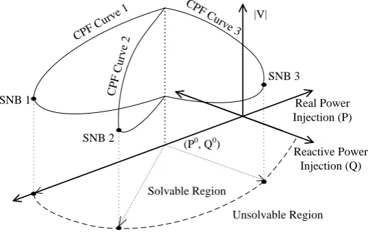
From the operating point, the CPF method finds the SNB point on a fixed direction of load increment. However, the different load directions produce different SNB points. A set of SNB points is the boundary of the solvable region, as shown in Fig. 1.

SNB 1

Reactive Power Injection (Q) Real Power Injection (P) |V|

(P0, Q0) CPF

Cu rve 3

SNB 3

SNB 2

Solvable Region

Unsolvable Region

CP F C

urv e 2

CPF C

urve 1

Fig. 1. Solvable boundary and CPF curves.

2.3. Tracing Boundary of Solvable Region: Continuation Method

g x_x( , ) y0 (6) y yT 1 (7)

where gx refers to the Jacobian matrix  g/ x of (5), y Nis the right eigenvector corresponding to

the zero eigenvalue of gx, and  p is a vector of load parameters with p designated as the number of

load parameters. The SNB point is the point that satisfies the system of nonlinear equations (5)-(7), which is

( )

1 T

 

 

_{ }   

 

0

x

g h z g y

y y

, (8)

where z





In this formulation, when p=1, the number of equations is 2N+1 and the number of variables is 2N+1. The solution is a SNB point that can be determined without creating the CPF curve.

For the solvable region visualization on the P-Q plane, the free parameters are the real and reactive power, this implies that p=2. Hence, the problem becomes 2N+2 variables with 2N+1 equations, the solution is a curve that can be traced by the continuation method. As shown in Fig. 2, the method in [12] applies the predictor-corrector process to trace the boundary curve. The predictor point is determined by moving the existing SNB point zn along the tangent vector v with the step size τ. The tangent vector v

can be obtained by:

n

 

Z Z Z

h v , (9) v 1, (10)

where hZ is the Jacobian matrix of (8). In the correction step, the next boundary point must satisfy (8)

and the following equation:

( ₁ )T 0

n  n  

z z v . (11)

Solvable Boundary n

z



v

z





v

1

n

z

Fig. 2. Solvable boundary tracing by continuation method.

2.4. Tracing Boundary of Solvable Region: Optimization-Based Method

Let S* be a vector of unsolvable power injections. For tracing the solvable region in [13], the minimization problem replaces the correction step as the following:

* *

,

1

min ( ) ( )

2

T

 

S x S S S S , (12)

s.t. ( )f x  S 0 , (13)

problem is to find the nearest solution point from the unsolvable point S*. According to the Kuhn-Tucker necessary condition, the solution to this problem is the singular point of the power flow Jacobian matrix [7]. At this point, the left eigenvector corresponding to the zero eigenvalue is a perpendicular vector of the solvable boundary. This vector is parallel to(SS*). The tangent vector v

for the predictor step can be obtained from

_(S_S*₎T_v_{0. (14)}

The solution obtained by (12), (13) is not a boundary point when S* is inside the region. As the solvable region is not always convex [14], [15], the modified predictor step determine the next S* by using the existing S*, as shown in Fig. 3.

* 2 S * 1 S

1 S

2 S

* 3 S

3

S S4

* 4 S 1

v

Fig. 3. Solvable boundary tracing by hybrid method.

3. Tracing Boundary of Feasible Region: Proposed Method

3.1. Feasible Region

₂

₁ Feasible Region

Infeasible Region Unsolvable Region

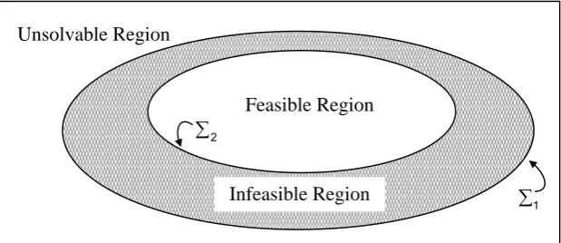
Fig. 4. Sets of operating points.

Figure 4 shows three regions of operating points bounded by the solvable boundary (₁) and the feasible boundary (₂). The unsolvable region is a set of operating points where the power flow equation has no solution. The infeasible region is a set of solvable operating points, but these points violate at least one operational limit. Finally, the feasible region is a set of solvable operating points where all system parameters are within their limits. This region is normally desirable for the operation. With the system condition consisting of the current load level and generator voltage schedule, the feasible boundary is traceable on the P-Q plane of considered bus.

3.2. Optimization Problem Formulation

 Power flow variables :

x[ _{pv pq} V_pq]T N (15)

 Free variables:

S_f [P Q _{g g} Q ]P_{c c} T ng2 (16)

The subscript “g” denotes the participant generator bus supplying the real and reactive power to the considered bus denoted by the subscript “c”. The number “ng” is a number of participant generator buses.

In this case, we consider only one load bus and try to plot the contour of feasible region within two-dimensional space between Pc and Qc. Therefore, power injections on other load buses are not taken

into account. The objective function is the reduced cost function as the following:

1





2 Pc Pc  Qc Qc (17)

The objective function is one half square of power mismatch that represents the distance between the infeasible point (P_c*,Q_c*) and the boundary point (Pc, Qc) by considering only the components of the

considered bus. It is also useful for tracing the outermost feasible region influenced by the load variation. The details describing this are introduced later.

The solutions have to satisfy power flow equations and all equipments have to operate within their limits. Thus, the constraints of this problem consist of:

 The power flow equality constraint:

( ,g x Sf)0 . (18)

 The load bus voltage limit:

min max

pq  pq pq

V V V . (19)

 The generator limit:

P_gmin P_g P_gmax, (20) Q_gmin Q_g Q_gmax. (21)

 The transmission line limit:

T x S( , f)ST, (22)

where T x S( , _f) : N ng 2 mis a function of the transmission line flows, S_T m is a vector of the transmission line limits, and m is a number of transmission lines.

 In the calculation, the real power injection of load bus is negative, that is:

P_c 0. (23)

For the particular load point * *

c c

Oppositely it returns the positive value when this load point is unfeasible, and the obtained solution is the nearest feasible point.

3.3. Tracing Algorithm

The algorithm for tracing the feasible region on the P-Q plane is described through the following steps: 1) Let S*( )_ci P_c*( )i  jQ_c*( )i be an infeasible load point. Select the load resulting in the violation as the

first infeasible load point;

2) Obtain the boundary point ( )i ( )i ( )i

c c c

S P  jQ by minimizing the objective function (17) subjected to constraints (18)-(23);

3) Obtain the direction w( )i by

( )i ₍ ( )i *( )i _{) (} ( )i *( )i ₎

c c c c

w  P P  j Q Q ; (24)

4) Determine the direction S*( )_ci by normalizing w( )i and then rotating 90 degrees counterclockwise by multiplying an imaginary unit j as the following,

S*( )_ci  jw( )i /w( )i ; (25)

5) Find the next infeasible point S*(_ci1) by a direction of S*( )_ci and a step size l as shown:

S*(_ci1) S*( )_ci   l S*( )_ci ; (26)

6) Repeat steps 2-5 to trace the boundary of feasible region until obtain the complete contour of feasible region.

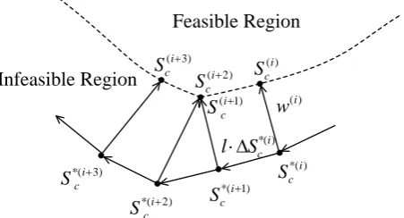
Because of the operational constraints, the feasible boundary may not be smooth at the point where two parts of different active constraints merge together. This tracing method repeatedly returns the same boundary point, the new S* changes positions around this boundary point until getting a new boundary point, as shown in Fig. 5.

Feasible Region

Infeasible Region

*( )i c S *(i 1)

c S  *(i 2)

c S  *(i 3)

c S 

( )i w ( )i c S

(i1)

c S  (i 3)

c

S  _{(i 2)} c S 

*( )i c lS

Fig. 5. Feasible boundary tracing.

3.4. Change of Feasible Region

The feasible boundary on the P-Q plane restricts the available area for the operating load. The varied load on the considered bus causes the operating point to move over inside its feasible region. Nevertheless, the shape of the feasible boundary is changeable by the parameters of other buses, e.g. the load variation, the capacitor bank operation, load shedding and generator voltage rescheduling.

P Q

Load shedding Reactive power

compensation Actions of other buses

Operating point

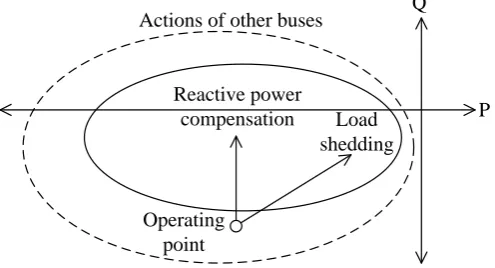
Fig. 6. Feasible region and operating point affected by control actions.

Figure 6 illustrates the effect of control actions on the P-Q plane. The control actions are capable of two ways, i.e. by driving the operating load back into the feasible region or by enlarging the feasible region [11]. The control actions studied in this article are the reactive power compensation and the load shedding.

As for the load bus, the installed capacitor banks can supply the reactive power and then bring the operating point back into the feasible region. If capacitor banks on that bus are not available, the capacitor banks operation on other buses can return the feasibility by reshaping the region. Furthermore, the load shedding is another control action to recover the undesirable situation. It can drive the operating point at that bus back to zero, and also reshape the feasible boundary on other buses because the load level in the system is reduced.

3.5. Feasible Region by Freeing Generator Voltages

The generator voltage setting is important for the power system operation. The tracing method in previous section determines the feasible region by setting generator voltages as constants. However, the generator voltages influence the shape of feasible region. Therefore, defining the generator voltages as unknowns is able to trace another type of feasible region. In this case, the vector of unknown variables in (15) is replaced by

x[ _{pv pq} V_pq V_g]T. (27)

The additional constraints for the optimization problem are the operational criteria of generator voltages (Vg), which is

V_gminV_g V _gmax . (28)

By minimizing the objective function (17) with the constraints (18)-(23) and (28) in the tracing process, the obtained region is the possibility of load by varying the generator voltages.

3.6. Outermost Boundary by Load Variation

Not only the generator voltage setting affects the feasible load region, the shape of boundary also depends on all power injections in the system. The outermost boundary point by the load variation can be determined by:

 As in the previous section, define the generator voltages as unknowns and bound it by the appropriate constraint.

S_f [ P Q]T. (29)

 For the load buses, the real power injections are normally negative by using the following constraints:

Ppq0, (30)

 Minimize the objective function (17) subject to (18)-(22), (28), and (30)

The optimization problem utilizes (17) to determine the outermost boundary of the considered bus. Although all loads in the system are free variables, the optimization problem can be solved to obtain the outermost boundary point of the considered bus because the target is to minimize the distance of apparent power only on that bus. The obtained boundary shows the potential of the system for supplying power to the considered bus.

4. Numerical Examples

This section visualizes the load feasible region by using the proposed method with the six-bus system [16] in Fig. 7, the system data are in Table 1-2. The criteria of generator voltages are assumed to be 1.05 pu for bus 1-2 and 0.97-1.07 for bus 3. The operation criterion of load bus voltage is 0.95-1.05 pu and the reactive power limit is 1.0 pu for every generator with 100 MVA base.

Table 1. Bus data.

Bus Bus type

Voltage (pu)

P (pu)

Q (pu)

Pgen min (pu)

Pgen max (pu)

Qgen min (pu)

Qgen max (pu)

Voltage limit (pu)

1 Swing 1.05 - - 0.50 2.0 -1.0 1.0 0.95-1.05

2 Gen 1.05 0.5 - 0.375 1.5 -1.0 1.0 0.95-1.05

3 Gen 1.07 0.6 - 0.45 1.8 -1.0 1.0 0.97-1.07

4 Load - -0.7 -0.7 - - - - 0.95-1.05

5 Load - -0.7 -0.7 - - - - 0.95-1.05

6 Load - -0.7 -0.7 - - - - 0.95-1.05

Table 2. Transmission line data.

From bus

To bus

Resistance (pu)

Reactance (pu)

Line charging susceptance

(pu)

Line limit (pu)

1 2 0.10 0.20 0.020 0.4

1 4 0.05 0.20 0.020 0.6

1 5 0.08 0.30 0.030 0.4

2 3 0.05 0.25 0.030 0.4

2 4 0.05 0.10 0.010 0.6

2 5 0.10 0.30 0.020 0.3

2 6 0.07 0.20 0.025 0.9

3 5 0.12 0.26 0.025 0.7

3 6 0.02 0.10 0.010 0.8

4 5 0.20 0.40 0.040 0.2

Bus 3 Bus 2

Bus 1

Bus 5

Bus 6

Bus 4

-P6,-Q6

-P5,-Q5

-P4,-Q4

Fig. 7. Six-bus test system.

4.1. Base Case Boundary Tracing

As a considered bus, bus 6 receives the power from all generators in the system. In this simulation, the first infeasible point S₆*(1) is equal to -j1.2 pu and the step size is 0.1 pu. The result in Fig. 8 shows the obtained boundary points of bus 6 and the infeasible points used for the tracing method. In the same way, the simulation also traces the feasible boundary of buses 4 and 5, as a result in Fig. 9. We observe that:

 Bus 5 has the greatest load margin in the direction of load increment with the same power factor.

 For bus 6, the point (0, 0) is outside the feasible boundary, the load shedding on bus 6 is therefore unavailable.

 Bus 4 has the greatest margin for the reactive power compensation.

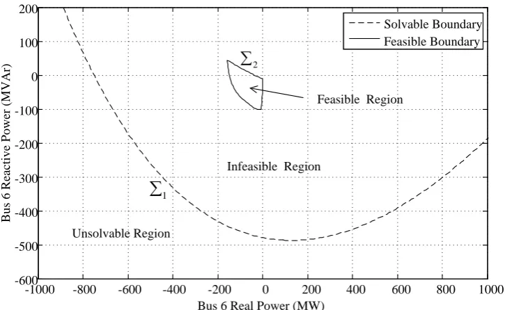
The obtained region is bounded by all operational limits. The boundary points are not necessary to be the singular points. Hence, this boundary is different from the solvable boundary. The result in Fig. 10 shows the load region of bus 6, the solvable region is much larger than the feasible region.

-200 -175 -150 -125 -100 -75 -50 -25 0 25 50 -150

-125 -100 -75 -50 -25 0 25 50 75 100

Bus 6 Real Power (MW)

B

u

s

6

R

ea

ct

iv

e

P

o

w

er

(

M

V

A

r)

Boundary Points Infeasible Points

-175 -150 -125 -100 -75 -50 -25 0 25 -125 -100 -75 -50 -25 0 25 50 75

Real Power (MW)

R ea ct iv e P o w er ( M V A r) Bus 4 Bus 5 Bus 6 Direction of Load Shedding Direction of Reactive Power Compensation (-70,-70) Direction of Load Increment

Fig. 9. Feasible regions of three load buses.

-1000 -800 -600 -400 -200 0 200 400 600 800 1000 -600 -500 -400 -300 -200 -100 0 100 200

Bus 6 Real Power (MW)

B u s 6 R ea ct iv e P o w er ( M V A r) Solvable Boundary Feasible Boundary Unsolvable Region

Infeasible Region

Feasible Region

2



1



Fig. 10. Feasible boundary and solvable boundary.

4.2. Effect of Reactive Power Compensation

-175 -150 -125 -100 -75 -50 -25 0 25 -150

-125 -100 -75 -50 -25 0 25 50

Bus 6 Real Power (MW)

B

u

s

6

R

ea

ct

iv

e

P

o

w

er

(

M

V

A

r)

Base Case Bus 4 at 0 MVAr Bus 5 at 0 MVAr

(-70,-70)

Load increment

Fig. 11. Feasible boundary change by reactive power compensation.

4.3. Effect of Load Shedding

Figure 12 compares the feasible regions of bus 6 in the case of: the base load, the load shedding at bus 4, and the load shedding at bus 5, respectively. The obtained result shows that the load shedding can improve the load margin, but the obtained region is smaller than that of the base case. Especially for the load shedding of bus 5, the upper part of the region significantly decreases. This implies that the operation of capacitor banks at this condition will bring about an unfeasible situation. Furthermore, the right part of the region also decreases because of the minimal limit of generators. The operating load of bus 6 can not be less than 60 MW, approximately.

-175 -150 -125 -100 -75 -50 -25 0

-125 -100 -75 -50 -25 0 25 50

Bus 6 Real Power (MW)

B

u

s

6

R

ea

ct

iv

e

P

o

w

er

(

M

V

A

r)

Base Case Bus 4 at 0 MVA Bus 5 at 0 MVA

(-70,-70)

Load increment

4.4. Effect of Generator Voltages

To study the effect of generator voltage setting, we define the generator voltages as free variables and then assign the constraint (28) to the optimization problem. The obtained boundary is the possibility of loading points under the control criteria of generator voltages. Figure 13 shows the feasible region with free generator voltages and then compares to the base case.

-175 -150 -125 -100 -75 -50 -25 0 25

-175 -150 -125 -100 -75 -50 -25 0 25 50 75 100 125 150 175

Bus 6 Real Power (MW)

B u s 6 R ea ct iv e P o w er ( M V A r)

Generator voltages are free to vary Generator voltages are fixed (base case)

Fig. 13. Feasible region when generator voltages are free to vary and feasible region of base case.

4.5. Effect of Load Level

-200 -175 -150 -125 -100 -75 -50 -25 0 25 -225 -200 -175 -150 -125 -100 -75 -50 -25 0 25 50 75 100 125 150 175 200

Bus 6 Real Power (MW)

B u s 6 R ea ct iv e P o w er ( M V A r) Base Case Heavy Load Light Load Variable Load

Fig. 14. Feasible boundary of bus6 change by load level.

Assume that:

Figure 14 illustrates the feasible boundaries from various load levels comparing with the outermost boundary (variable load) obtained by the method in section 3.6. The region is large in the case of light load and small in the case of heavy load. However, we can observe that the region in the case of light load is cut by the minimum limit of generator, i.e. the load lower than approximately 12 MW is not feasible. Furthermore, the outermost boundary covers all three feasible regions. It displays the potential of the system to supply load at bus 6.

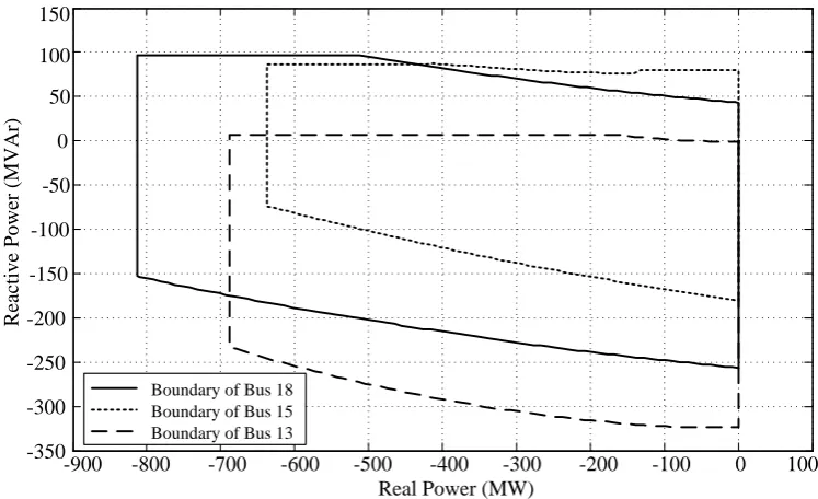
4.6. Larger Test System

In this section, the IEEE-24 bus test system [17] is the larger system chosen to illustrate the robustness of the proposed algorithm. The considered buses are bus 18, bus 15 and bus 13, which have the top three largest loads in this system. The load feasible regions are determined by the proposed method, as shown in Fig. 15.

-900 -800 -700 -600 -500 -400 -300 -200 -100 0 100 -350

-300 -250 -200 -150 -100 -50 0 50 100 150

Real Power (MW)

R

ea

ct

iv

e

P

o

w

er

(

M

V

A

r)

Boundary of Bus 18 Boundary of Bus 15 Boundary of Bus 13

Fig. 15. Load feasible regions evaluated from IEEE-24 bus system.

5. Conclusion

The boundary of feasible region is important for determining the robustness of operating points. The feasible region is the set of power flow solutions without any operational violation. This paper proposes the method for tracing the feasible boundary of the considered load bus. The optimization-based method is able to solve the feasible boundary point by assigning free variables and the operational limits. The modified predictor-corrector process can trace the feasible boundary and obtain the complete contour of feasible boundary in the two-dimensional space.

References

[1] V. Ajjarapu and C. Christy, “The continuation power flow: a tool for steady state voltage stability analysis,” IEEE Transaction on Power Systems, vol. 7, no. 1, pp. 416-423, Feb. 1992.

[2] H. D. Chiang, A. J. Flueck, K. S. Shah, and N. Balu, “CPFLOW: A practical tool for tracing power system steady-state stationary behavior due to load and generation variations,” IEEE Transactions on Power Systems, vol. 10, no. 2, pp 623-634, May 1995.

[3] C. A. Canizares and F. L. Avarado, “Point of collapse and continuation methods for large AC/DC systems,” IEEE Transactions on Power Systems, vol. 8, no. 1, pp. 1-8, Feb. 1993.

[4] Y. V. Makarov, D. J. Hill, and Z. Y. Dong, “Computation of bifurcation boundaries for power systems: a new ∆-plane method,” IEEE Transactions on Circuits and Systems, vol. 47, no. 4, pp. 536-544, Apr. 2000.

[5] C. A. Canizares, “Calculating optimal system parameters to maximize the distance to saddle-node bifurcations,” IEEE Transactions on Circuits and Systems-I: Fundamental Theory and Applications, vol. 45, no. 3, pp. 225-237, Mar. 1998.

[6] R. J. Avalos, C. A. Canizares, F. Milano, and A. J. Conejo, “Equivalency of continuation and optimization methods to determine saddle-node and limit-induced bifurcation in power systems,” IEEE Transactions on Circuits and Systems., vol. 56, no. 1, pp. 210-223, Jan. 2009.

[7] T. J. Overbye, “ A power flow measure for unsolvable cases,” IEEE Transactions on Power Systems, vol. 9, no. 3, pp. 1359-1365, Aug. 1994.

[8] T. J. Overbye, “Computation of a practical method to restore power flow solvability,” IEEE Transactions on Power Systems, vol. 10, no. 1, pp. 280-287, Feb. 1995.

[9] S. N. Singh and S. C. Srivastava, “Corrective action planning to achieve a feasible optimal power flow solution,” IEE Proceedings Generation, Transmission and Distribution, vol. 142, no. 6, pp. 576-582, Nov. 1995.

[10] S. Granville, J. C. O. Mello, and A. C. G. Melo, “Application of interior point methods to power flow unsolvability,” IEEE Transactions on Power Systems, vol. 11, no. 2, pp. 1096-1103, May 1996.

[11] A. G. C. Conceicao and C. A. Castro, “A new approach to defining corrective control actions in case of infeasible operating situations,” IEEE Porto Power Tech Conference, Sep. 2001.

[12] I. A. Hiskens and R. J. Davy, “Exploring the power flow solution space boundary,” IEEE Transactions on Power Systems, vol. 16, no. 3, pp. 389-395, Aug. 2001.

[13] Y. Yu, P. Li, H. Jia, S. T. Lee, and P. Zhang, “Computation of boundary of power flow feasible region with hybrid method,” in Proceedings of Power Systems Conference and Exposition, IEEE PES, New York, vol. 1, pp. 137-143, Oct. 2004.

[14] B. C. Lesieutre and I. A. Hiskens, “Convexity of the set of feasible injections and revenue adequacy in FTR markets,” IEEE Transactions on Power Systems, vol. 20, no. 4, pp. 1790-1798, Nov. 2005.

[15] Y. V. Makarov, Z. Y. Dong, and D. J. Hill, “On convexity of power flow feasibility boundary,” IEEE Transactions on Power Systems, vol. 23, no. 2, pp. 811-813, May 2008.

[16] A. J. Wood and B. F. Wollenberg, Power Generation Operation and Control, New York: John Willey & Sons, 1996, pp. 123-124.