White Rose Research Online URL for this paper:
http://eprints.whiterose.ac.uk/1544/
Article:
Moss, G E and Runciman, C orcid.org/0000-0002-0151-3233 (2001) Inductive
benchmarking for purely functional data structures. Journal of Functional Programming.
pp. 525-556. ISSN 1469-7653
https://doi.org/10.1017/S0956796801004063
[email protected] https://eprints.whiterose.ac.uk/ Reuse
Items deposited in White Rose Research Online are protected by copyright, with all rights reserved unless indicated otherwise. They may be downloaded and/or printed for private study, or other acts as permitted by national copyright laws. The publisher or other rights holders may allow further reproduction and re-use of the full text version. This is indicated by the licence information on the White Rose Research Online record for the item.
Takedown
If you consider content in White Rose Research Online to be in breach of UK law, please notify us by
c
2001 Cambridge University Press
Inductive benchmarking for
purely functional data structures
GRAEME E. MOSS and COLIN RUNCIMAN
Department of Computer Science, University of York, York, UK
Abstract
Every designer of a new data structure wants to know how well it performs in comparison with others. But finding, coding and testing applications as benchmarks can be tedious and time-consuming. Besides, how a benchmark uses a data structure may considerably affect its apparent efficiency, so the choice of applications may bias the results. We address these problems by developing a tool for inductive benchmarking. This tool, Auburn, can generate benchmarks across a wide distribution of uses. We precisely define ‘the use of a data structure’, upon which we build the core algorithms of Auburn: how to generate a benchmark from a description of use, and how to extract a description of use from an application. We then apply inductive classification techniques to obtain decision trees for the choice between competing data structures. We test Auburn by benchmarking several implementations of three common data structures: queues, random-access lists and heaps. These and other results show Auburn to be a useful and accurate tool, but they also reveal some limitations of the approach.
1 Introduction
In recent years, many papers have given details of new functional data structures (Chuang & Goldberg, 1993; Okasaki, 1995a; Okasaki, 1995b; Okasaki, 1995c; Brodal & Okasaki, 1996; Erwig, 1997; O’Neill & Burton, 1997). However, these papers give only limited attention to empirical performance. Okasaki writes in an open problems section of his thesis, ‘The theory and practice of benchmarking [functional] data structures is still in its infancy’ (Okasaki, 1996b). This paper develops the theory and practice of benchmarking functional data structures.
1.1 Overview of Auburn
We address these problems by developing a tool, calledAuburn, for benchmarking functional data structures. Auburn works with the signature of an abstract datatype (adt), such as the signature for lists in figure 1 of section 2, and with one or more
Haskell implementations of theadt.
Among other things, Auburn can automatically generate a range of pseudo-random benchmark tests making use of a given adt. Auburn can run these tests using each implementation, apply an inductive classification procedure to the results, and derive a decision tree for the appropriate choice of implementation depending on the application. By generating a fair distribution of benchmarks over a wide variety of different uses, we not only find which data structure is best overall, but also which data structures are best for particular uses.
To apply a decision tree one needs a profile characterising how the adtis to be used. Auburn can also extract such a profile from any application program making use of anadt. Even if we have a single application of anadtin mind, measuring its
performance for each possible implementation could be tedious, and would still not give us any understanding of how theadtis being used or why performance differs
as it does between implementations. By applying a decision tree to the application’s profile, we can predict the best choice of data structure and have a way to understand the choice.
The key technical idea on which Auburn is based is the datatype usage graph
(dug) – a detailed representation, using a labelled directed multi-graph, of how
a program makes use of an adt. All the benchmark tests Auburn constructs are
represented asdugs, and interpreted by specially-generated evaluators for eachadt.
(Interpretive overheads are determined by generating null implementations, and subtracted appropriately from the measures of the actual implementations.) How an application uses an adtis also recorded as adug.
A profile of adt usage is actually a vector of attributes characterising a (large)
family of dugs. For example, attributes include the relative frequencies of different
operations. Determining the profile of a dug is easy; generating valid dugs from
profiles is much harder, and unless all theadtoperations are total, the programmer
has to supply extra information with a signature and its implementations. However, the extra information can also be used to improve decision trees.
Auburn is implemented mainly in Haskell, with a supporting library in C. The implementation is freely available fromhttp://www.cs.york.ac/fp/auburn/.
1.2 Overview of this paper
This paper is based on the first author’s thesis (Moss, 1999), to which readers are referred for a more comprehensive account. For example, the thesis includes a full review of all the data structures we have investigated, and a full description of how Auburn is implemented. Here we are necessarily selective.
defines aDatatype Usage Graph(dug) recording how a data structure is used by an
application, and a profile summarising the most important aspects of adug.
Section 3 describes the core algorithms of Auburn. These involve the creation of benchmarks from profiles through the generation and evaluation of dugs, and
the extraction of profiles from applications through the extraction and profiling of
dugs.
Section 4 explains how Auburn induces decision trees for the choice of different implementations in different parts of dug-space.
Section 5 reports the results of applying Auburn to various implementations of three different adts: heaps, queues and random-access sequences. We assess the accuracy of Auburn’s results and investigate the sources of any inaccuracy.
Section 6 concludes with a summary and pointers to related and future work.
2 Datatype Usage Graphs
2.1 Abstract datatypes
An abstract datatype (adt) provides operations to create, manipulate and observe
values of some new type. The only way to interact with values of this type is through theadtoperations. This restriction allows theimplementation of theadtto
be isolated from its use – we may change implementations without changing how we use theadt.
We shall restrict ourselves to container types, i.e. adts that contain elements of
some other type. For example, a list adt allows lists of integers, lists of characters, etc. For any such adt, we may consider theadt as defining a type constructor T.
For example, a list adt may be taken as defining a type constructor List taking a type t to the type List t. A list of integers would then have the type List Int. We shall restrictT to be unary. Most commonadts satisfy these restrictions.
Definition 1 (adt)
For any type constructorT, and any set of functionsF, the pair (T , F) is anadtif
the following conditions are satisfied: • T is unary.
• Each function inF takes at least one argument of typeT a, or returns a result of typeT a, wherea is a type variable.
As a further simplification, we restrict ourselves tosimple adts, according to the
following definitions. Many adts are simple: queues, deques, lists, random-access
sequences, heaps, sets, integer finite maps, etc. However, any higher-order operations, such asmap, or any operations converting from one data structure to another, such asfromList, are excluded.
Definition 2 (Simple Type)
moduleList (List,empty,cons,isEmpty,head,tail,catenate,lookup)where
empty :: List a
cons :: a→List a→List a isEmpty :: List a→Bool head :: List a→a tail :: List a→List a
catenate :: List a→List a→List a lookup :: List a→Int→a
Fig. 1. The signature of a simple listadtAList, expressed in Haskell. The exported type
constructor isList, and the type of each operation is simple overList.
fully,simple over T) iftcan be formed astype by the grammar
type ::= argument type→type |result type argument type ::= T a |a |Int
result type ::= T a |a |Int |Bool
wherea is a type variable, andtcontains at least one occurrence ofT a.
Example 2
The following types are simple over the type constructors Queue, List and Set
respectively:
• Queue a→a →Queue a
• List a→Int →a
• Set a
Definition 3 (Simple adt)
We define theadtA= (T ,{f1, . . . , fn}) to be simpleif the type of each operationfi
is simple over T.
Example 3
The signature of a simpleadtAList is given in figure 1, expressed in Haskell. During the run of an application, many different instances of an adt will exist. Each of these particular instances of the adtis called aversion (Okasaki, 1998).
Definition 4 (Generator, Mutator, Observer, Role, Version Arity)
The role of any operation f of type t1 → t2 → · · · → tm, simple over the type
constructorT, can be classified as follows.
Generator: tm=T aand (∀j,16j < m)tj6=T a
Mutator: tm=T aand (∃j,16j < m)tj=T a
Observer: tm6=T aand (∃j,16j < m)tj=T a
Theversion arityof an operation is the number of version arguments it takes. Every generator has version arity 0, and every mutator and observer has version arity >1.
Example 4
2.2 Usage graphs
To model how an adt is used by an application we use a labelled directed multi-graph. The nodes are labelled with partial applications of the adt operations to
specific values for all the non-version arguments: for simplicity, these are restricted to atomic values. The version arguments are recorded as arcs from other nodes that compute them: there is an arc fromutov if the result of the operation atuis taken as an argument by the operation at v. The nodes are also numbered according to the order of evaluation. Such a graph is called aDatatype Usage Graph (dug).
A node of a dugis called aversion node if it is labelled with an operation that results in a version. The subgraph of a dug containing just the version nodes is
called theversion graph.
We express these ideas more precisely in the following definitions.
Definition 5 (Partial Application, Pap(A))
Given a simple adt A= (T ,{f1, . . . , fn}), apartial application of fi is any function
of the following form:
λx1·λx2·. . .·λxk·fia1 a2 . . . am, 06k6m
Here, m is the arity of fi, each version argument xj occurs exactly once in the
sequence [a1, . . . , am], and all the other elements of this sequence are atomic values
such as integers. To avoid duplication, we further insist thatx1,. . . ,xk occur in order
in the sequence [a1, . . . , am]; that is,xioccurs beforexj fori < j. The set of all partial
applications of any function of a simple adtAis denoted byPap(A).
Example 5
For the list adt AList, whose signature is given in figure 1, the following functions are in Pap(AList):
• λl·cons ’a’l
• empty
• λl1·λl2·catenate l1 l2
We may use a partial application to assign a role to a node: For a node v labelled with a partial application of the operation f, the role ofv is defined to be the role of f.
We are now in a position to give a definition of adug. For nodes with more than
one incoming arc, we need to identify which arc corresponds to which argument. We therefore label every arc with an argument position.
Definition 6 (dug)
Given a directed multi-graph G = (V,E), a simple adt A = (T ,{f1, . . . , fn}), a
total mapping η:V →Pap(A), a bijectionσ:V → {1..|V|} and a total mapping
τ:E →N, the 4-tuple (G, η, σ, τ) is a dug forA, if for everyv ∈ Vthe following
properties are satisfied:
1. The arity ofη(v) equals the in-degree ofv.
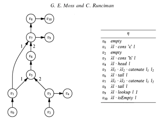
Fig. 2. Adugfor the listadtAList.
3. If the incoming arcs tov, ordered byτ, have sourcesv1, . . . , vk, then the types of
arguments required byη(v) match the types of results supplied byη(v1), . . . , η(vk).
4. Ifvhas successor w∈ V, thenσ(v)< σ(w).
5. The type of every argument ofη(v) isT a, for some uniform instantiation ofa. Properties 1–3 ensure the dug is well-defined. Properties 4–5 impose restrictions
on dugs to make generating dugs easier: Property 4 orders the arguments of an operation before the operation itself, forcing the graph to be acyclic – see the problemChoosing the operation before the arguments of section 3.1.1 for justification of this restriction; Property 5 ensures only version arguments are taken from the results of other operations – see the problem Choosing non-version arguments of section 3.1.1 for justification.
Example 6
Figure 2 shows an example of a dug. A table defines η. The ordering σ of the
evaluation of the nodes is given byσ(vi) =i. For nodes of in-degree>1 the labels
assigned by τare written beside the relevant arcs:v5 catenatesv1 onto the front of
v3, andv7 catenatesv1 onto the front ofv6. The type variablea can be instantiated
to the typeChar to obtain type consistency for every function application.
2.3 Evaluation
We have so far presented a dugas a record of how an application uses an imple-mentation of anadt. We can reverse this process. By creating anevaluator of dugs,
we create an artificial slice of the application that uses anadtimplementation in the
same way. We can then use this slice as a benchmark with a known pattern of use. We definedug evaluation more precisely by first defining how we may associate
each node with a function application.
Definition 7 (Interpretation of Partial Applications)
Let A be any simple adt. Let f be an operation of A. Let g ∈Pap(A) be any
partial application off. LetIbe an implementation ofA. The interpretation of g
under I, denoted by [[g]]I, is the value ofg using the implementation off inI.
Example 7
Let Lbe the ordinary Haskell implementation of lists, then • [[λl·cons True l]]L =\l→(True:l)
• [[λl·head l]]L=\(x:xs)→x
• [[empty]]L=[ ]
Definition 8 (Interpretation of Nodes)
Let (G, η, σ, τ) be any dug for the adt A, let v be any node of G, and let I be
an implementation of A. Let the arcs incident to v, ordered by τ, be from the nodes v1, . . . , vk respectively. The interpretation of v under I, denoted by [[v]]I, is
the following expression:
[[v]]I= [[η(v)]]I [[v1]]I . . . [[vk]]I
where the right-hand side is an application of the function [[η(v)]]I. Note that asG
is acyclic, this recursive definition is sound.
Example 8
Using the dug shown in figure 2, and the ordinary Haskell implementation L of
lists,
• [[v1]]L =(\l→(’c’:l)) [ ]
• [[v4]]L =(\(x:xs)→x) ((\l→(’h’:l)) [ ]).
2.3.1 Order of evaluation
The order of evaluating the interpretations of thedugnodes can significantly affect efficiency. Within functional languages there are two main schemes for deciding the order of evaluation of an expression: lazy and eager. We can accommodate either scheme by using the node orderingσ of adug(G, η, σ, τ) in different ways, but here
we consider only one.
demand the values that are of some other type. Looking at adug, only the values
given by the observer nodes have such a type. The order in which we demand these values may affect efficiency, but for simplicity we assume that the order of evalua-tion for observer nodes coincides with the order of formaevalua-tion for their associated closures.
Definition 9 (Lazy Evaluation of a dug)
Given a dug (G, η, σ, τ) for an adt A, and an implementation I of A, the lazy evaluation of the dug with respect to Iis the process of performing the following
steps on each nodeσ(i) in order: • Form the closure given by [[σ(i)]]I.
• If the node is an observer, demand the value of this closure.
Example 9
The lazy evaluation of thedugof figure 2 would form the closures [[vi]] for 06i610 in order. When the closures for the observer nodes are formed, namely [[v4]], [[v9]], and [[v10]], their values are demanded at the same time.
2.4 Profile
We want to create a benchmark from a dug, and we want to extract a dug from
an application. However, a dug may be too large and complex to serve as an intelligible pattern of use. So we next define the profile of a dug. The profile will
condense the most relevant characteristics of aduginto a few numbers. We can use
pseudo-random numbers to generate a family of dugs thaton average have a given profile. The initial seed given to the pseudo-random number generator determines which one is chosen.
So what characteristics do we choose to record in a profile? A distinctive property of purely functional data structures is that their operations are non-destructive; but the extent to which applications depend on this property varies greatly. So one component we choose to include in a profile is the fraction ofpersistentapplications of operations. An application of an operation is persistent if one of the version arguments has already been mutated—that is, a mutator has already been applied to this argument.
Definition 10 (Mutation, Observation)
For any node v of the version graph of adug, amutation ofv is an arc from v to
a mutator node. Note that an n-ary mutator creates n mutations. An observation is defined similarly. Mutations and observations inherit the ordering given to the nodes towhich they point.
Example 10
Figure 2, the arc from v7 to v8 is a mutation, and the arc from v7 to v9 is an observation. As v9 is ordered after v8, the observation v7 →v9 is ordered after the mutation v7→v8.
Definition 11 (Persistent, Original)
For any node v of the version graph of adugwith node ordering σ, a mutation or
observation ofv ispersistent if it is ordered byσ (andτ)after the earliest mutation
of v. A mutation or observation that is not persistent is calledoriginal.
Example 11
In figure 2, we see that the observationv7→v9occurs after the mutationv7 →v8. As this mutation is the only mutation ofv7, it is also the earliest. Thus the observation
occurs after the earliest mutation, and so is persistent. The mutationv1→v7is also persistent. The observation v3→v4 is original.
A more obvious characteristic of dugs is the ratio of how many times we apply one operation relative to another.
Definition 12 (Weight)
For any dug D, theweight of a mutator f in D is the number of mutations that apply fto nodes inD. The weight of an observer is defined similarly. The weight of a generator f is simply the number of nodes that are generated byf.
Example 12
The weights of the operations in the dugin figure 2 are:
Operation : empty catenate cons tail head lookup isEmpty
Weight : 2 4 2 2 1 1 1
Generative power of profiles. Information such as the average number of mutations of a node is not only useful for summarisingdugs, it also provides a very convenient
way to generate adugwith a given profile.
From the fraction of mutations that are persistent, we can calculate the average number of mutations of previously mutated nodes as follows. Letpmbe the fraction
of mutations that are persistent. Take any node vi that is mutated at least once.
The first mutation of vi is original, and the remaining ni mutations are persistent.
Averaging over all jmutated nodes, we have
pm=
Pj i=1ni
Pj
i=1(ni+ 1)
, n=
Pj i=1ni
j ⇒ n=
pm
1−pm
If we know the fraction m of version nodes that are not mutated at all, we can calculate the average numberµof mutations of a node:
µ= 0m+
1 + pm 1−pm
(1−m) = 1−m 1−pm
We callpmthepersistent mutation factor (pmf), andmthemortality.
If we calculate the ratio r of mutations to observations, we can also estimate the average number of observations of a node. Under the simplifying assumption that a node was made by a mutator, the average number of observations of a node is 1/r. As we have excluded nodes made by generators, this number is only an estimate. From the fraction po of observations that are persistent, we can calculate
and the average number of observations made after the first mutation atpo/r. We
call po thepersistent observation factor (pof).
We separate generation weights from the weights of mutators and observers. To allow the calculation of the ratio r of mutations to observations, we group the mutation and observation weights together to form themutation-observation weights. The ratio of generations to other operations is governed by mortality and by the persistence factors.
Definition 13 (dugProfile)
The profile of a dugDwith version graphGV is given by the following:
• Generation weights: The ratio of the weights of each generator.
• Mutation-observation weights: The ratio of the weights of each mutator and observer inGV.
• Mortality: The fraction of nodes in GV that are not mutated.
• pmf: The fraction of mutations of nodes inGV that are persistent.
• pof: The fraction of observations of nodes inGV that are persistent.
Example 13
Thedugshown in figure 2 has the following profile:
• Generation weights: As there is only one generator, empty, this property is redundant:empty = 1.
• Mutation–observation weights: We have
catenate:cons :tail :head :lookup:isEmpty= 4 : 2 : 2 : 1 : 1 : 1 Note that each application ofcatenatecarries double the weight of an application of one of the other operations because each application ofcatenate creates two mutations.
• Mortality: Of the eight version nodes, only one (v8) is not mutated, so the mortality is 1/8.
• pmf: There are eight mutations, one of which (v1→v7) is persistent, so the pmf
is 1/8.
• pof: There are three observations, one of which (v7 → v9) is persistent, so the
pofis 1/3.
If thepmfandpofof adugare both zero, then we know that there are no persistent
applications of an operation. Therefore, we make the following definition.
Definition 14 (Single-Threaded)
An application using an implementation of a simple adt A in a manner recorded
by thedugDissingle-threaded (with respect toA) if thepmfandpofofDare both zero. A single-threaded application does not require a persistent implementation of theadt.
Example 14
The part of the dugin figure 2 restricted to nodesv0, . . . , v6 has pmf=pof=0 and is
2.5 Shadow data structure
To aid the generation of dugs, and to add information to profiles, we use ashadow data structure. A shadow data structure maintains a shadow of every version. This shadow contains information about the version. A shadow data structure does not depend on a specific implementation of theadt; it is applicable to any
implementa-tion of theadt. A shadow data structure is only used for the generation or analysis
of dugs, and need not be involved in applications using anadtimplementation. As a running example, for the adt AList, whose signature is given in Figure 1,
and for which each version is a list, let the shadow of a version contain the length of the list.
Guarding against undefined applications. When generating adug from a profile, if we blindly choose to label a node with any operation, we may create an application that is undefined: for example, the head of an empty list. Such applications ofpartial operations need to be excluded from aduggenerated at random. We need to have a
guard around the partial operation telling us which applications of the operation we can form. We can use the shadow of a version to store enough information to allow decisions about whether a particular operation may be applied to that version. For example, for AList, if we maintain the length of a list in the shadow, we can restrict
the use of an operation such as taking the head of a list, applying it only to lists of positive length.
Shadow Profiling. The shadow can also store any other useful information about what operations were performed. This shadow profile allows information specific to an adt to be collected. For example, by maintaining the length of a list, we
can calculate the average lengths of lists passed to each mutator or observer. This extra source of profiling information is important. Without it, for example, ‘N
insertions followed by N deletions’ and ‘N insertions each followed by a deletion’ have indistinguishable profiles. IfN is large, the ideal implementation is unlikely to be the same in each case.
To simplify the definitions that follow, we shall assume that each occurrence of the type variable a in the type of an ADT operation is instantiated to Int. This assumption also simplifies both duggeneration anddugextraction,
Definition 15 (Shadow Operation)
For any simpleadt (T , F), and for any generator or mutator f ∈F, let t be the
type of f with type variable a instantiated to Int. For any type s, the function g
is an s-shadow of f if g has the type shadows(t), derived from t by replacing all
occurrences ofT Int bys. The shadows maintained by this shadow operation have type s. There are no shadows of observers as they do not return versions.
Example 15
For any types, an s-shadow of theupdate operation of AList (see figure 1) has the
following type:
Definition 16 (Shadowing)
Let A = (T ,{f1, . . . , fn}) be any simple adt. Without loss of generality, let
{f1, . . . , fm} be the generators and mutators of A. For any set F′ = {f1′, . . . , f′m}
of operations, and any type s, the pair (s, F′) is ashadowing ofA if the following hold for alli∈ {1, . . . , m}:
• The operationfi′is ans-shadow of fi.
• There exists a homomorphismφ::T Int→s; that is, for allx1, . . . , xk, wherek
is the arity offi, iffix1 . . . xk is well-defined, then
φ(fix1 . . . xk) =f′i (φ′ x1) . . . (φ′ xk)
where for allx,
φ′ x=
φ x, if x has type T Int x, otherwise
Example 16
In one possible shadowing SList of AList the type sshadowing List Int is of type Int, and the homomorphism φ :: List Int →Int is the function that returns the length of a list.
Definition 17 (Shadow Evaluation)
Let Dbe any dugforadt A, and S= (s, F) be any shadowing ofA. Theshadow
evaluation ofDis a mappingζthat takes a version nodevto the result of evaluating [[v]]S, where an operation is interpreted by its shadow.
Example 17
Taking thedugof Figure 2 with a shadowingSList tracking list length, the shadow
evaluationζ of thedug is:
vi : v0 v1 v2 v3 v5 v6 v7 v8 ζ(vi) : 0 1 0 1 2 1 2 1
2.5.1 Guarding
For each operation f we need to define a guard that indicates which applications of f are allowed. We could make a guard take the same arguments as f, but with shadows for versions, and return true or false, according to whether the application is allowed or not. However, this approach has the disadvantage of forcing a choice of all arguments before applying the guard. For an operation such as indexed lookup, we have to guess which indices are appropriate before testing the validity of the application – hardly efficient.
The definition of a dug already restricts arguments supplied by the result of
non-version argument is of type Int, each domain of legitimate values for such an argument is a subset of the integers, for which the following definitions assume a suitable representation typeIntSubset.
Definition 18 (Guard Type)
Let T be any type constructor of arity one. Let tbe any simple type overT with type variableainstantiated toInt. Letnbe the number of arguments of an operation of type t, v of which are version arguments. For any type s, the type guards(t) is given by
guards(t) =
v times
z }| {
s→ · · · →s→
[IntSubset]n−v ifv < n
Bool ifv=n
where [a]mis the type of lists ofmelements of typea, and wheresrepresents the type
of shadows. Every version argument is replaced by a shadow, and every non-version argument moves over to the result type. There are n−v non-version arguments; if
n−v= 0, then the result type isBool, otherwise it is a list ofn−velements each of type IntSubset.
Example 18
Consider the adt AList, whose signature is in figure 1. For any type s, a guard of
the operationhead using shadows of typesmust be of type
guards(List Int →Int) =s→Bool
If we add the operation update of type
update::List a→Int →a→List a
toAList, then any guard ofupdate must be of type
guards(List Int →Int →Int→List Int) =s→[IntSubset]2 Definition 19 (Guard)
Let S= (s, F′) be a shadowing of theadt A= (T , F) defining a homomorphism
φ::T Int →s. For any operationf ∈F of typet, the functiong is anS-guard of
f if the following hold: • The type ofg isguards(t).
• For allx1, . . . , xn, wherexi1, . . . , xik are each of typeT Int and
xj1, . . . , xjl are the rest, we have:
— Ifl= 0,f x1 . . . xn is well-defined if
g (φ xi1) . . . (φ xik) =True
— Ifl>1,f x1 . . . xn is well-defined if
g (φ xi1) . . . (φ xik) = [xs1, . . . ,xsl]
and for all 16t6l,
To generate adug:
whilethedugis too smalldo
choose an operation
choose version arguments for the operation choose non-version arguments for the operation add a node to thedug
add arcs from the nodes used as arguments to the new node label the node with the operation and the remaining arguments
Fig. 3. Initial outline of a simpleduggeneration algorithm.
Example 19
The guards for head and tail applied to shadow-length s return s6= 0. The guard forlookup returns [{1. . . s}].
3 Implementing DUGs
3.1 From profile to benchmark
We derive a benchmark from a profile in two stages:
(1) A dug generator uses pseudo-random numbers to create a dug that
proba-bilistically has the given profile, i.e. theexpected profile is the one given. (2) Adugevaluator executes this dugusing a given implementation of theadt.
3.1.1 dugGeneration
How shall we build a dug? Figure 3 gives a reasonable starting point for an
algorithm, but proceeding along these lines one encounters various problems. • Creating undefined applications. Some applications of operations may not be
well defined. For example, the applicationhead empty is usually not defined. We avoid these applications by maintaining extra information – a shadow – about each possible argument of an application. A guard protects us from creating an undefined application, by using the shadow of every argument. • Allowing undefined arguments. Lazy evaluation evaluates the operation, not
the arguments. Therefore, adding a node with (as yet) undefined arguments seems reasonable. However, without knowing the arguments, we cannot avoid undefined applications using a shadow data structure. So we never add a node without knowing all the arguments.
• Choosing the version arguments.We could pick the arguments from any part of thedugalready formed. But as we must maintain a shadow of every possible
• Choosing non-version arguments.How can we generate an argument of typea? As no profile properties depend on non-version arguments, we restrict them to integers—that is, we instantiate the type variable atoInt. We then choose all non-version arguments independently of the graph.
• Choosing the operation before the arguments.If each operation is chosen before any arguments are selected, it is hard to make a generated dug conform to
some of the profile properties. It is easier if for each new node we plan a sequence of operations it should be involved in as an argument, and for each operation maintain a version-argument buffer of the appropriate arity. We place nodes in the buffer for their next planned operation. When a buffer is full, we create a new node accordingly, emptying the buffer.
• Diverging. If we allow the same operation and arguments to be chosen re-peatedly, and if this application is rejected by the guard, we could diverge. Therefore, once a guard rejects an application, we revise the plans for argument nodes, skipping this operation.
A refined outline of theduggeneration algorithm is given in figures 4 and 5. We build a dug one node at a time. Each node has a future and a past. The future
records which operations we have planned to apply to the node, in order. The past records which operations we have already applied to the node. The nodes with a non-empty future together make up the frontier. The first operation in a future is called thehead operation.
As we add a node to the dug, we take arguments from the frontier. We bound
the size of the frontier above and below:
• Bounding above prevents the frontier from getting too large. If the pmf is
non-zero, we shall need to mutate nodes more than once, leading to continual growth of the frontier. So we cap the frontier size to prevent running out of memory. When the frontier exceeds a given limit, we remove an arbitrary node from the frontier.
• Bounding below ensures there is at least one node to build on, and encourages diversity, especially in the presence of operations with large version arities. When a new node is created, we record this event as a birth. A list of births, in order, describes a dug completely. When a node no longer has a future, we record its past as adeath. A list of deaths also describes adugcompletely. A list of births
is more convenient for evaluating adug, whereas a list of deaths is more convenient
for profiling adug. So we produce both.
3.1.2 dug Evaluation
The process of dugevaluation is comparatively straightforward. Unlikedug
gener-ation, we encounter no theoretical problems, only the practical one of efficiency. Our first dugevaluator required more time for input-output and maintaining a lookup
table than foradtoperations, preventing us from accurately measuring their relative
To generate adug:
whilethedugis too smalldo ifthe frontier is too smallthen
try to make a new node using a generator (*)
else-ifthe frontier is too largethen
remove a node from the frontier record the death of this node
else
remove a node from the frontier to act as a version argument
place the node in the buffer corresponding to the node’s head operation
if this buffer is fullthen
try to make a new node with the buffer’s contents acting as the version arguments for their common head operation (*)
fi fi od
record the death of every node in the frontier and buffers
Fig. 4. Overview of theduggeneration algorithm (Part I). Further details of steps marked
(*)are given in the next figure.
use an extension to the Green Card package to support calls from C to Haskell (Peyton Joneset al., 1997).
An overview of the evaluation algorithm is given in figure 6. When a non-version node is born, its result must be demanded immediately. As the result of an observer is either of typeIntor of typeBool, we demand this value by converting it to an integer, and adding it to thechecksum. This checksum is the result of the dug evaluation.
Different implementations of the sameobservationally-equivalent adtevaluating the
same dug should return the same checksum; so by comparing checksums we can
check the results of one implementation against those of another.
3.2 From application to profile
3.2.1 dugExtraction
The task of extracting adugfrom the run of an application is quite tricky in a lazy
language like Haskell. One approach is to modify the compiler. However, as this solution depends on the details of a specific compiler, it would not be portable. An alternative approach is to transform the original program into one that gives the same result, but also produces adug. We adopt this method.
Problems of dugExtraction. Here are two key goals we must achieve by
transform-ing the original program:
To try to make a new node from an operation and some version arguments: apply the guard of the operation to the shadow of every version argument
if the guard succeedsthen
choose some non-version arguments from the result of the guard make a new node by applying the operation to the arguments record the birth of this node
add the new node to thedug
ifthe operation is not an observerthen
plan the future of the new node
else
leave the future of the new node empty
fi
ifthe new node has a non-empty futurethen
add the new node to the frontier
else
record the death of this node
fi fi
remove the head operation of each version argument
record the death of every version argument with an empty future add remaining version arguments to the frontier
Fig. 5. Overview of theduggeneration algorithm (Part II).
whilenot at the end of thedugfiledo
read the next birth or death
if it is a birththen
apply an operation to integers and nodes in the frontier, as given by the birth
ifthe operation is an observerthen
convert the result to an integer and add it to the checksum
else
add the resulting node to the frontier
fi else
remove the dead node from the frontier
fi od
report the checksum
Fig. 6. Overview of thedugevaluation algorithm.
Some arguments may not be evaluated at all; after the program has finished, we record any such unevaluated arguments explicitly in thedug.
• Recording the dug. We must record the dug as output, but do not wish to
transform every function to work within the IO monad. Neither do we wish to accumulate information about the dugby extending the result from every
dataTwa = Node Int(T a)
fw
i :: wT(ti,1)→ · · · →wT(ti,ni)
fw
i a1 . . . ani−1=
letnodeId = new nodewN(fi)
inseq nodeIdwR(fi wA(a1) . . . wA(ani−1))
where
wT(t) =
Twa, if t=T a
t, otherwise
wN(fi)gives the data constructor that namesfi
wR(e) =
Node nodeIde, if e has typeT a
e, otherwise
wA(aj) =
arc aj nodeId j, if ajhas type Twa
intArg aj nodeId j, if ajhas type Int
aj, otherwise
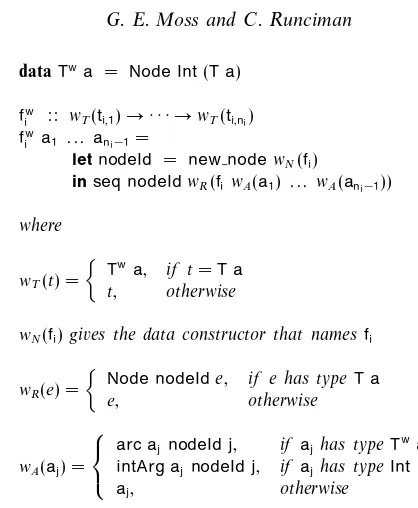
Fig. 7. Definition of a wrappedadt. For anadtexporting type constructorTand operations
fi :: ti,1→ · · · →ti,ni, the wrappedadtexports type constructorTwand operationsfiw.
We cannot, however, record arguments of type a, as we do not know in general how to store these. The user could supply a function to convert any value of typeato, say, an integer. However, extracting this value could evaluate the argument more than previously. Therefore we do not record values of such arguments.
How dug Extraction is Done. We modify the application and adtimplementation
to perform the same task, but produce a dug as a side-effect. The modification
involves wrapping the main function and everyadt operation. The wrapped main function performs some initialization, calls the old main function, and then tidies up the results. Each wrapped adt operation works with wrapped versions. A version is wrapped with an identity tag. A wrapped operation uses the identity tags to record, each time it is called, which nodes supply its version arguments. A wrapped operation also calls the old operation, and wraps the result into a node with a new identity tag.
The rules for deriving a wrapped adt are given in figure 7. For example, the wrapped version of aListdatatype is
dataWrappedList a = Node Int (List a)
and the wrapped implementation ofconsis
wrappedCons :: a→WrappedList a→WrappedList a wrappedCons i v =letnodeId = new node Cons
[image:19.595.182.391.112.366.2]The functionarcunwraps and returns the version argument, after recording the arc from this version node to the newly created node.
arc :: WrappedList a→NodeId→Int→List a
arc (Node from v) to position = seq from (seq (new arc from to position) v)
The functions new nodeand new arcare implemented in C; new nodereturns a new identity tag for a node, after recording which operation labels this new node, whereas new arcreturns only unit, after recording the arc, including the argument node identity, the result node identity, and the position of the argument node.
Evaluation of wrappedConsoccurs only when cons would have been evaluated in the original program. It forces the evaluation of the identity of the new node, and then returns the wrapped result. However, we do not record any of the arguments yet, as we do not know that they will be evaluated. We wrap the version argument with a call to arc. When the version argument would have been evaluated by the original program, we can examine the identity of the argument.
3.2.2 dugprofiling
As with dug evaluation, we read one birth or death at a time. The algorithm is
quite straightforward. The type of a profile is
dataProfile = Profile{generationWeights :: [(Operation,Weight)],
mutationObservationWeights :: [(Operation,Weight)], mortality :: Double, pmf :: Double, pof :: Double}
To calculate the generation weights and the mutation-observation weights, we keep a note of the number of nodes made by each operation. To calculate the mortality, we accumulate both the number of nodes not mutated, and the total number of nodes. From this information we can calculate the proportion of nodes not mutated: that is, the mortality. Similarly, we accumulate integer numerators and denominators to calculate thepmfand thepof.
4 Inductive classification of benchmarks
Our goal is a tool that gives benchmarking results qualified by the pattern of datatype usage. Naively we might hope to create a benchmark with every possible pattern of use – using some discrete scale for profile values – and provide a lookup table of times of each implementation running each benchmark. The user simply obtains the pattern of use of their application, and looks up the quickest implementation in the appropriate row of the table. Unfortunately, this approach is not practical. Such a table would cover a huge number of points, and the total time to collect the results for each point would be far too large, because the number of patterns of use is exponential in the number of usage attributes.
4.1 Decision trees
Of the many possible approaches to the problem of characterising the key attributes, our chosen method is to induce a decision tree(Quinlan, 1986). For our purposes, a decision tree is a binary tree with the following properties:
• Each branch node is labelled with a test of the form A 6 v, where A is a datatype usage attribute, andvis some constant.
• Each leaf node is labelled with the name of anadtimplementation.
Decision trees can be used to choose an implementation given knowledge of datatype usage: start at the root and follow the appropriate branches till you reach a leaf.
A decision tree is induced from a training set of the data it is to characterise. In our case, this training set is a sample of benchmarks. The sample is generated from a random selection of attribute values, but it is the attributes of the resulting benchmarks that are used, thereby including the attributes both of the profileand of the shadow profile– an important source of extra information. Each benchmark in the sample is run, and the performance of each implementation is recorded. From these results, we induce a decision treeT. Given any benchmarkBfrom the sample, using only the attributes of B, T will decide upon the winning implementation. More generally, given a sufficiently large and varied sample, the decision tree induced should be able to predict the winning implementation of any benchmark with good accuracy.
4.2 Induction algorithms
We take an existing algorithm from the literature for inducing a decision tree from a sample. We use the algorithmc4.5 (Quinlan, 1993), which is a descendant of id3
(Quinlan, 1986). Both algorithms are widely known and respected in the machine learning community.
The basic idea underlying c4.5 is a simple divide and conquer algorithm due to
Hunt et al. (1966). Let S be the results of running a sample of benchmarks. Let
I1, . . . , Ik be the competingadt implementations. There are two cases to consider:
• Scontains only results reporting a single implementationIjas the winner. The
decision tree forS is a single leaf labelled withIj.
• S contains results reporting a mixture of winners. By dividingS into S1 and
S2 according to some test, we can recursively construct treesT1 andT2 from S1 andS2 respectively.
The key to a good implementation of Hunt’s algorithm is the choice of test with which to splitS. The set of possible tests is limited by the range of attribute values for benchmarks in S. Let [v1, . . . , vn] be the distinct values, in order, of an attribute
A for benchmarks in S. Consider two consecutive values, vi and vi+1. For any v
satisfying vi 6 v < vi+1, splitting S with the test A 6 v results in the same split.
But how do we choose which test to use at each stage?id3uses thegain criterion
to measure the quality of a test, whereasc4.5 uses thegain ratio criterion(Quinlan, 1993). We have tried both, but the results reported in section 5 are for the gain ratio criterion, as it proved more successful.
4.3 Simplifying decision trees
The decision tree induced by this method classifies the results of the given sample
perfectly. Unfortunately, this tree is not an ideal basis for choosing an implementation for two reasons: (1) the tree may be very large and complex; (2) the tree is based on the chosen sample and may be over-specific. Therefore we prune the induced tree: wherever replacing a subtree with either one of its children or with a single leaf does not increase the predicted error of the subtree, it is pruned to this smaller tree.
There is a choice of methods for error prediction (Quinlan, 1987; Quinlan, 1993). Some are based on further test samples: for example, if in addition to recording the winning implementation for the test we also record the ratio of the time of
every implementation to the time of the winning implementation, one definition of the predicted error of a subtree is the average ratio of the implementation given by the subtree as the winner. However, we found that a statistical pruning method described by Quinlan as ‘far more pessimistic’ (Quinlan, 1993) works just as well without requiring further tests.
5 Results
In this section we present some results from the use of Auburn1 to evaluate over
twenty different data structures implementing queues, random-access sequences and heaps.
Queues Among the simplest of adts, queues have the following signature.
empty :: Queue a
snoc :: Queue a→a→Queue a
head :: Queue a→a
tail :: Queue a→Queue a
In addition to a naive implementation of queues as lists, we take the batched and
multihead variants of a pair (Hood & Melville, 1981), two refinements of list-pairs justified by the banker’s model (Okasaki, 1996c) and the physicist’s model (Okasaki, 1998) of amortized complexity, a real-time variant of banker’s queues (Okasaki, 1995c), and Okasaki’s bootstrapped andimplicit queues (Okasaki, 1998).
1All the benchmark tests reported here were compiled using the York nhc13 byte-code Haskell compiler,
Random-access sequences We use the term random-access sequence to describe a list
adtthat also supports indexed lookup and update, with the following signature.
empty :: RASeq a
cons :: a→RASeq a→RASeq a
head :: RASeq a→a
tail :: RASeq a→RASeq a
lookup :: RASeq a→Int→a
update :: RASeq a→Int→a→RASeq a
Besides anaivelist implementation, we takethreaded skew binarylists (Myers, 1983), Adams’ balanced trees (Adams, 1993), Braun trees (Hoogerwoord, 1992), slowdown deques (Kaplan & Tarjan, 1995) restricted to the relevant operations, skew binary
lists (Okasaki, 1995b) andelevator lists (Moss, 1999).
Heaps A heap is an ordered collection of elements, with the following signature.
empty :: Ord a⇒Heap a
insert :: Ord a⇒a→Heap a→Heap a merge :: Ord a⇒Heap a→Heap a→Heap a findMin :: Ord a⇒Heap a→a
deleteMin:: Ord a⇒Heap a→Heap a
Once again we include a naive implementation using (ordered) lists. The other implementations arebinomialheaps (Okasaki, 1998),skew binomialandbootstrapped skew binomial heaps (Brodal & Okasaki, 1996),pairingheaps (Okasaki, 1996a),leftist
heaps (N ´u˜nez et al., 1995) andsplay heaps (Okasaki, 1998).
5.1 Performance measures
We apply the terms score and cost to implementations or decision trees with the following meanings.
Definition 20 (score,cost)
Given a set of implementations for an adt Aand a set of benchmark tests using
A, we define the scoreobtained by each implementationI to be the percentage of tests for whichIis fastest, and the (normalised)cost ofIto be the average across all tests of the ratios between the execution time for I and the execution time of the fastest implementation for each test.
If usage attributes are known for each test, a score and a cost can also be assigned to a decision tree, based on the percentage of tests for which the implementation selected by the tree is the fastest, and on the ratios between the execution times for the implementation selected by the tree and the fastest implementation for each test.
Example 20
5.2 Correctness checks and fine-tuning
Tracing Bugs. Before we benchmark the implementations, we ensure that we have coded them correctly. Although type checking catches most accidental errors, some may remain. It is also possible that an implementation presented in the literature contains a mistake. We can use Auburn to check that implementations of the same adt produce the same results. Auburn can generate a series of
pseudo-random dugs, searching for the smallestdugthat causes an error: that is, either an implementation fails to evaluate the dug– for example, because of a run-time error
– or two implementations return different checksums. The benchmarker outputs any anomalousdugas a Haskell program. In the 23 initial implementations, we detected
4 faults this way. The smaller the dug, the easier it is to find the bug. So in each
case we let the benchmarker run for a long time, trying to find the smallest failing
dug. For example, the queue benchmarker found a subtle bug in our bootstrapped
queue implementation. The smallest failing dug– discovered after a run of several hours – has 22 nodes.
Fine-Tuning. Coding an implementation involves many low-level design decisions, some of which can make a significant difference to performance. Auburn helps us to make such design decisions because it can compare the overall performance of an implementation with and without a minor modification. We use the benchmarker of each adt to time each implementation and its variants over a sample of 100 benchmarks. For each variantIthe benchmarker reports the score and cost of the ‘decision tree’ made from a single leaf I – the tree that always choosesI. Guided by comparisons of these scores and costs, we made nine improvements to our initial implementations, each gaining between 4% and 63% in performance.
5.3 Decision trees and their performance
For eachadt, after fine-tuning the implementations, we apply the inductive
bench-marker to a training sample of 200 pseudo-randomdugs.
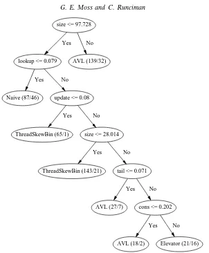
5.3.1 Analysis of the random-access sequence decision tree
The most accurate decision trees are too large to show and discuss here, but figure 8 shows a simplified tree for random-access sequences. Each leaf is annotated with (N/E), where N is the number of benchmarks in the test sample covered by this leaf, and E is the number of misclassifications by this leaf. The significance of a leaf can be estimated from the number and proportion of winning implementations that it classifies correctly. Almost all of the leaves have a low proportion of errors. The Elevator leaf has a high proportion of errors, and the remaining leaves on the subtree from the test tail 60.071 show AVL to win over half of the cases (36 out of 66). We consider the other leaves in turn.
size <= 97.728
lookup <= 0.079 Yes
AVL (139/32) No
Naive (87/46) Yes
update <= 0.08 No
ThreadSkewBin (65/1) Yes
size <= 28.014 No
ThreadSkewBin (143/21) Yes
tail <= 0.071 No
AVL (27/7) Yes
cons <= 0.202 No
AVL (18/2) Yes
[image:25.595.148.450.111.477.2]Elevator (21/16) No
Fig. 8. A decision tree induced using the gain criterion on a training sample for the random-access sequenceadt, pruned using a reduced error method.
logarithmic complexity. The AVL implementation benefits from balancing specialised to adding or removing an element at the left, i.e. fromcons ortail. It is not clear if the Adams implementation could use a similar improvement. • Fair size, small lookup weight (Naive).This decision is a little surprising. If few
update operations are done, then we would expect the Naive implementation to win. But what if there are quite a lot ofupdateoperations? We might expect the Naive implementation to lose. The leaf’s annotation does show quite a few errors, but there is another reason: Anupdatewill be fully evaluated only if it is forced. The only observations in the absence of lookup are head and
isEmpty, and because the Naive implementation is so lazy, these observers will force updates only on the first element. The other implementations are not as lazy, and so do not benefit as much.
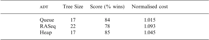
Table 1. The performance of decision trees induced by Auburn from a sample of 200
dugs and applied to a distinct test sample of 500 dugs. The size of a tree is the
number of branch nodes
adt Tree Size Score (% wins) Normalised cost
Queue 17 84 1.015
RASeq 22 78 1.093
Heap 17 85 1.045
ThreadSkewBin implementation deliberately implements an efficient lookup
operation, at the expense of an inefficientupdate operation.
• Small size, fair lookup weight, fair update weight (ThreadSkewBin). Although ThreadSkewBin implementsupdate to takeO(i) time, where i is the index of the element updated, for small lists, it competes well with the log-time AVL implementation. The simplicity of the ThreadSkewBin implementation makes it win on small lists, even with manyupdate applications.
• Fair size, fair lookup weight, fair update weight (AVL). With enough update
operations, and a reasonably sized sequence, the AVL implementation beats the ThreadSkewBin implementation.
For a similar analysis of decision trees for Queues and Heaps see Moss (1999).
5.3.2 Usage-based decision vs. single implementation
One way to assess the quality of the decision trees induced by Auburn is to collect a further, larger sample of benchmarks for eachadt, and to examine the accuracy
of the decision trees by applying them to these unseen test cases. For each of the threeadts, Table 1 shows the scores and costs of the induced decision tree applied
to a test sample of 500dugs.
Do we gain anything by choosing an implementation according to the datatype usage? How do the implementations chosen by a usage-based decision tree compare with the single implementation chosen simply because it has performed best overall in previous tests?
For queues, the Batched implementation wins for 72% of the tests and has a normalised cost of just 1.02. So it seems that for these implementations of thisadt
there is little to gain by choosing the implementation according to datatype usage – one could just choose the Batched implementation regardless. However, with a score of 84% and a cost of 1.015, the decision tree does manage to improve on the fixed choice of a Batched implementation.
Similarly for heaps, the Pairing implementation wins for 80% of tests with a normalised cost of 1.08 and would make a good fixed choice. Still, the decision tree increases the score to 85%, and reduces the cost to 1.045.
the Elevator implementation has the lowest overall cost (2.12). By selecting imple-mentations to match usage, the decision tree scores 78% and reduces the cost to 1.093 – far better than any uniform choice of a single implementation.
5.3.3 Real applications
So we can use Auburn to produce advice about the choice of implementation for at least threeadts. But how good is this advice in practice? To answer this question,
we construct severalreal benchmarks – real in that they produce useful results. We time each benchmark with each implementation and compare the results against Auburn’s prediction, based on an extracted profile of the benchmark. We take four benchmarks for eachadt, and four data sets for each benchmark.
Random-Access Sequence Benchmarks. Again we give details only for random-access sequences. An array is one of the most commonly used data structures, even in functional programs, so benchmarks are not hard to find. However, we also wish to include algorithms that use the sequences as lists, as in Okasaki (1995b).
• Bucketsort. This sort uses random-access operations heavily, see Cormen et al. (1990, p. 180).
• Quicksort. This functional implementation of Quicksort (Hoare, 1962) does not use any random-access operations.
• Depth-First Search (DFS). Implementing a graph as a random-access list of adjacent vertices (Cormen et al., 1990, p. 465) allows any graph algorithm to use random-access lists. We choose one of the simplest graph algorithms, depth-first search (Cormenet al., 1990, p. 477).
• Kruskal’s Minimum-Cost Spanning Tree (KMCST).Kruskal implements a min-imum cost spanning tree algorithm (Cormen et al., 1990, p. 504) using a disjoint-set data structure (Cormen et al., 1990, p. 440), which we implement using a random-access list.
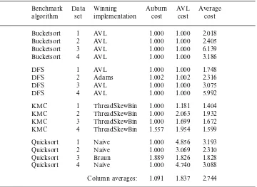
Table 2 gives the results. The costs of the implementations predicted by Auburn’s decision trees are given alongside costs for the single implementation with the best overall performance (the least cost of any fixed choice of implementation regardless of datatype usage), and the average cost across all implementations (the expected cost of a randomly selected implementation).
Even the best uniform choice (of AVL trees) has a normalised cost of 1.837, indicating that the performance of implementations varies significantly across the benchmarks. Auburn’s predictions perform significantly better on average than this uniform choice, and far better than a random choice.
Across all three adts, we found that Auburn gave good advice for all the real
Table 2. Results from real applications of random-access sequences
Benchmark Data Winning Auburn AVL Average
algorithm set implementation cost cost cost
Bucketsort 1 AVL 1.000 1.000 2.018
Bucketsort 2 AVL 1.000 1.000 2.405
Bucketsort 3 AVL 1.000 1.000 6.139
Bucketsort 4 AVL 1.000 1.000 3.186
DFS 1 AVL 1.000 1.000 1.748
DFS 2 Adams 1.002 1.002 2.316
DFS 3 AVL 1.000 1.000 3.075
DFS 4 AVL 1.000 1.000 5.992
KMC 1 ThreadSkewBin 1.000 1.181 1.404
KMC 2 ThreadSkewBin 1.000 2.063 1.932
KMC 3 ThreadSkewBin 1.000 1.699 1.672
KMC 4 ThreadSkewBin 1.557 1.954 1.599
Quicksort 1 Naive 1.000 4.856 3.193
Quicksort 2 Naive 1.000 3.069 2.310
Quicksort 3 Braun 1.889 1.826 1.828
Quicksort 4 Naive 1.000 4.740 3.088
Column averages: 1.091 1.837 2.744
5.4 Locating inaccuracy in Auburn
So Auburn’s advice is good, but not perfect. What can go wrong? We briefly examine the main sources of possible inaccuracy.
5.4.1 Insufficient dug
Does the dugmodel capture datatype usage sufficiently? To answer this question,
we apply the following test. Take all the real application benchmarks, and run each using eachadtimplementation, measuring the efficiency. Extract thedugfrom each
run. Evaluate eachdugusing the corresponding adtimplementation. Compare the
efficiencies of the implementations when used by the application with the efficiencies of the implementations when used by thedugevaluators.
If thedugcaptures all of the relevant information for influencing the efficiency of anadtimplementation, we would expect the relative efficiencies of the
implementa-tions to be the same. For example, the order of the implementaimplementa-tions, most efficient first, should be the same for the application as for the dug evaluator. Further, the
efficiencies should correlate linearly.
For each comparison of relative efficiencies of implementations, we calculate the
Table 3. Mean correlation coefficients when comparing real benchmarks with evaluation of dugs generated from the benchmark profile
adt dug& Benchmark dug&dug
Queue 0.859 0.923
RASeq 0.704 0.969
Heap 0.694 0.999
by not recording actual element values. Instead element values are generated pseudo-randomly, and the only constraint that can be specified is the range from which they are drawn. The impact is minor foradts whose operations do not depend heavily
on comparisons of elements, but more marked for something like a heap in which order is of intrinsic importance.
5.4.2 Insufficient profile
Just as we design the dug to capture datatype usage, we design the profile of a dug to capture those aspects of datatype usage that most affect implementation
efficiency. We base the whole of Auburn on this premise. We test its validity by generating several dugs from the same profile and comparing the performance of
implementations evaluating the different dugs. If the profile of adugdoes capture datatype usage sufficiently, then the results should be similar. To avoid limiting the test to pseudo-random dugs generated using Auburn, we extract the original profiles from real benchmarks. Table 3 shows the results. The correlation between
dugs generated from the same profile is very high for each adt. However, the
correlation between the benchmark and the generated dugs is significantly lower
– though still quite high. This difference indicates that some important aspects of datatype usage in a benchmark are not being carried through a profile into a generateddug. One important factor is the lack of size information: although size
is captured in the profiling information, and figures prominently in decision trees, it does not influenceduggeneration.
5.4.3 Strictness Issues
When an implementation evaluates adug, only the observations are demanded. As a result, some of the generations and mutations may not be forced, depending on the strictness of theadtimplementation evaluating thedug.
To estimate the average proportion of a dug not evaluated, we evaluate sample dugs for each of the three adts, queue, random-access sequence, and heap, and
all of their implementations. For each dug D0, we extract the dug D1 actually
evaluated – by transforming a dug evaluator for dug extraction, as described in
iteration: D1 =D2. Comparing the profile of D0 with the profile of D1, averaging
across all of the dugs of the three adts, each of the weights differ by less than
0.01, the mortality differs by about 0.05, thepmfdiffers by about 0.01, and thepof
differs by about 0.35. So only the pof differs greatly. It differs because neitherdug
evaluation nor dug extraction preserve the order of evaluation of mutations, only
the order of evaluation of observations.
5.4.4 Inaccurate or over-specific trees
Some of Auburn’s predictions of the best implementations for the real benchmarks are quite inaccurate. One reason for these inaccuracies is a constraint on induced decision trees. More accurate trees of similar size might employ tests on arithmetic
combinations of attributes. However, as Quinlan (1993, Sect. 10.2) points out, intro-ducing the possibility of such tests can slow down the process of induction by an order of magnitude.
Conversely, the very exactness of some binary decisions can be unhelpful if the expected range of values for some attribute of an application crosses a critical threshold. Recording normalised costs as well as simple scores is a help – both for programmers consulting a decision tree directly, and for pruning methods used to eliminate over-specific tests.
6 Conclusions, related and future work
Summary of contribution Previous approaches to benchmarking functional data structures have relied on hand-picked benchmarks, giving results biased towards an unknown datatype usage. This paper has described a way to automate the pro-duction of results qualified by a description of datatype usage, as implemented in theAuburn toolkit. The main contributions are
• A formally defined model, adug, of how an application uses an adt. • A method for extracting adugas a slice of an application.
• The definition of dug profiles, summarising the most importance aspects of dugs in vectors of numeric attributes.
• A method for creating adug, and hence an artificial benchmark application,
from a profile of intended usage.
• The application of inductive classification to performance data for a pseudo-random sample of dugs, deriving decision trees for the choice of data struc-tures.
• Results of applying Auburn to over twenty data structures, implementing three differentadts.
Despite various limitations in the way dugs and their profiles are defined and