Meshless Method Based on Moving Kriging Interpolation for Solving Simply Supported Thin Plate Problems

Article

Meshless Method Based on Moving Kriging

Interpolation for Solving Simply Supported Thin

Plate Problems

Supanut Kaewumpai

Department of Management, Martin de Tours School of Management and Economics, Assumption University of Thailand, 88 Moo 8, Bangna-Trad Rd., Samutprakarn, 10540, Thailand

E-mail: [email protected]

Abstract. Meshless method choosing Heaviside function as a test function for solving simply supported thin plates under various loads as well as on regular and irregular domains is presented in this paper. The shape functions using regular and irregular nodal arrangements as well as the order of polynomial basis choice are constructed by moving Kriging interpolation. Alternatively, two-field-variable local weak forms are used in order to decompose the governing equation, biharmonic equation, into a couple of Poisson equations and then impose straightforward boundary conditions. Selected mechanical engineering thin plate problems are considered to examine the applicability and the accuracy of this method. This robust approach gives significantly accurate numerical results, implementing by maximum relative error and root mean square relative error.

Keywords: Meshless method, moving Kriging interpolation, thin plate bending problems, biharmonic equation, irregular domain.

ENGINEERING JOURNAL Volume 19 Issue 3 Received 27 May 2015

Accepted 27 May 2015 Published 5 June 2015

1.

Introduction

The structures of plate are one of the important components in various applications. There are many scientists or researchers who have analyzed these structures. Exact analysis for such a plate is usually very difficult, in spite of the existence of analytical solution in some special cases of geometry and loads. Therefore, various numerical methods have been developed. Meshless methods have become very attractive and efficient for development of adaptive methods for solving thin plate bending problems. The main advantage of meshless methods is to get rid of or at least alleviate the difficulty of meshing and re-meshing the entire plate structure. For analysis of thin plate bending, it is well known that high order derivatives of field variables in the governing equation give rise to difficulties in solution of boundary value problems because of worse accuracy of numerically evaluated high order derivatives. The order of the differential operator can be decreased mathematically by decomposing this operator into two lower order differential operators with introducing new field variables. To circumvent the problems associated with meshing, a number of works for plates have been investigated based on meshless methods. Meshless methods can be traced back to 1977 when Lucy, Gingold and Monaghan [1] proposed a smooth particle hydrodynamics (SPH) method that was used for modeling astrological phenomena without boundaries, such as exploding stars and dust clouds. Krysl and Belytscho [2] first employed the element free Galerkin method (EFGM) to analyze the thin plate problems while Liu Gu [3] introduced the idea of moving Kriging interpolation (MK) and show how it can be used to formulate a new type of meshless method in heat conduction problems. In 1998, the meshless local Petrov-Galerkin (MLPG) method was first proposed by Atluri and Zhu [4], [5]. This method has been applied widely and very successfully in recent years. This method is based on moving least squares (MLS) approximation for construing nodal shape function and used the local weak formulation for substituting the trial function transformed into the discretized system of linear equations. The main advantage of this method is that it only requires nodes and a description of the external and internal boundary conditions, therefore, no element connectivity, neither total nor part, is needed. Effective implementations of MLPG method are keys to success [6], [7], [8], [9]. Three years later, Long and Atluri [10] extended the meshless local Petrov-Galerkin (MLPG) for solving thin plate bending problems. Sladek et al. [11] applied the new field variable for solving thin plate bending problems by meshless method based on the moving least squares approximation (MLS) and point interpolation approximation. Recently, Kaewumpai et al. [12], [13] presented two-field-variable meshless method based on polynomial augmented radial point interpolation for solving thin plate problems with subjected to boundary of the second kind. All of these meshless methods do not need an element mesh for the interpolation of the field or boundary variables. The purpose of this paper is to present the meshless method with two-field-variable local weak form for solving simply supported thin plate problems subjected to various loads as well as regular and irregular domains. Moving Kriging interpolation is employed to construct the nodal shape function choosing the Heaviside step function is used as the test function. Selected numerical examples are considered comparing with exact solution which measured with the maximum of relative error and root mean square of relative error.

2.

Moving Kriging Interpolation

Moving Krigking interpolation (MK) can be extended to any sub-domain   x . Generally, the MK interpolation w

 

x is defined by









  

1

( ) N _i( ) _i ( ) ,

i

w x x w Φ x W x

(1)

T T

( ) ( )  ( )

Φ x p x A r x B

and the shape function Φ x( ) is defined by

 T  T

( ) ( ) ( ) ,

Φ x p x A r x B

(2)

where p x( )is a complete monomial basis:





 

T

1 2

( ) p( ) p ( ) p_m( ) ,

p x x x x

(3)

and Wis fictitious values:

_wˆ( )₁ wˆ( )₂  wˆ( _N) ._

  

₍ T 1 ₎1 T 1_,

A P R P P R

(5)



 1(  ).

B R I PA

(6)

The matrices

P R

,

and_{r x}T

 

_{are given as follow:}

    _            1 2 1 2 1 2 ( ) ( ) ( ) ( ) ( ) ( ) , ( ) ( ) ( ) m m m

p p p

p p p

p p p

1 1 1

2 2 2

N N N

x x x

x x x

P

x x x

(7)              _            ( , ) ( , ) ( , ) ( , ) ( , ) ( , ) ( ) , ( , ) ( , ) ( , )

1 1 1 2 1 N

2 1 2 2 2 N

N 1 N 2 N N

x x x x x x

x x x x x x

R x

x x x x x x

(8)



  



 

T_{( ) ( , ) ( , ) ( , ) ,}

1 2 N

r x x x x x x x

(9)

and Iis an identity matrix.



( ,x xi j) is the dimensionless correlation Gaussian function between any pair

of nodal points located at xi andxj, namely

    2 ( ) ( , ) , ij c r d e i j

x x

(10)

where r_ij  xixj ,  0 is the dimensionless shape parameter and dc is a characteristic length that is related to the nodal spacing in the local domain of the point of interest.

3.

Thin Plate Bending Equation and Discretization

3.1. Governing Equations

In the classical Kirchhoff's theory of bending of thin plates [9], the governing equation which results in the biharmonic equation may be written as

4_{w( )}q( ) _,

D

x

x x

(11)

where

w

( )

x

is the plate deflection,

q

( )

x

is the prescribed load normal to the plate,

  

    

   

4 4 4

4

4 2 2 4

( ) 2

x x y y is a biharmonic operator, and Dis the flexural rigidity. The plate domain

 

[0,1] [0,1]



is enclosed by the following simply supported boundary conditions edge:

                2 2 2 2 2 2 2 2 (0, )

(0, ) 0 ; 0,

(1, )

(1, ) 0 ; 0,

( ,0)

( ,0) 0 ; 0,

( ,1)

( ,1) 0 ; 0.

w y w y x w y w y x w x w x y w x w x y

(12)

 2

( ): ( ),

m x w x

(13)

2_{m( )} q( )_.

D

x

x

(14)

3.2. Discretization

Using the local weighted residual method, Eq. (13) and Eq. (14) become







   



2 _0,

i s

i

w m v d

(15)



_{ }  _{ }

 

 



2 _0,

i s

i

q

m v d

D

(16)

where vi is the test function choosing as the Heaviside step function. Applying the Green’s first identity in Eq. (15) and Eq. (16), the following local weak forms can be obtained

 



   







0,

i i

s s

w_{d md}

n

(17)

 



   







0.

i i

s s

m q

d d

D

n

(18)

Next, transverse deflection w and a new variable m are interpolated by using MK; consequently, the following discrete equation for each node is obtained

                   _  _{ }     _{ }    _  _{ }    _{ }             









1 1 ˆ ( )

( ) ₀

ˆ , ˆ ( ) 0 ˆ i i s s i s i s j i j i N j i N w d d w q m d d D m x x n x n

(19)

where

i j

,



1,2, , .



N

4.

Numerical Examples

In this section, some numerical results are presented to verify this approach which compare to an exact solution by investigating the accuracy and convergence as well as computational efficiency of presented formulation and technique. The accuracy of numerical solutions is illustrated by plotting the selected number of nodal points versus the maximum relative error as well as root mean square relative error in tests of accuracy of approximation for deflections at evaluation. Both of errors were defined as:



_max max

|

w w_exactexact

|

,























1

2

( )

( )

1

.

( )

exact N

k k

rms exact

k k

w

w

N

w

x

x

x

(21)

[image:5.595.130.450.282.748.2]

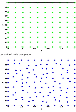
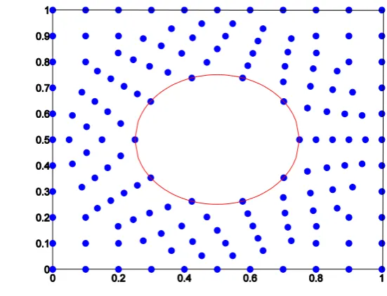
First of all, the linear and quadratic bases are chosen in order to construct nodal shape function by using moving Kriging interpolation. In all the following examples, correlation parameter is set as 0.5 for being a smooth curve while the radius of each local subdomain should be big enough such that the union of all local subdomains covers as much as possible in order to avoid singularity of calculated matrices. For this reason, the radius of the local subdomain of each boundary node is taken as 0.7 times minimum nodal points while 21 Gaussian points are used on each section of boundary edge Conventional nodal and unconventional arrangements are chosen as 16(4x4), 25(5x5), 36(6x6), 49(7x7), 64(8x8), 81(9x9), 100(10x10), 121(11x11), 144(12x12), 169(13x13) and 196(14x14) on domain for each example. Illustratively, selected 10x10 conventional nodal arrangement and 11x11 unconventional nodal arrangements are shown in Fig. 1 and Fig. 2, respectively.

Fig. 1. 10x10 conventional nodal arrangement.

[image:5.595.140.451.521.737.2]

4.1. Sinusoidal Load on a Simply Supported Square Plate

An exact solution in term of deflection is given by

 

 



0

4 2

2 2

( , ) sin sin ,

1 1

(

)

q x y

w x y

a b

D

a b

(22)

where q0 represents the intensity of the load at center of the plate, D is the flexural rigidity and a b, are

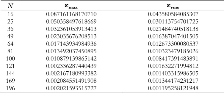
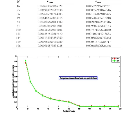
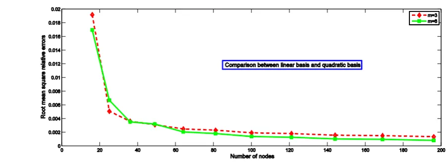
the side length of a rectangular plate. The fictitious values w versus exact solution and absolute value of the difference between exact solution and approximate solution is shown in Fig. 3. Tabular errors using linear basis and quadratic basis for nodal shape construction of Example 4.1 are shown in Table 1 and Table 2, respectively. According to both tables, these results show the convergence of this method by increasing the number of nodal points. In addition, illustratively, the results of absolute maximum relative errors and root mean square relative errors are plotted as a function of nodal points are shown in Fig. 4 and Fig. 5, respectively.

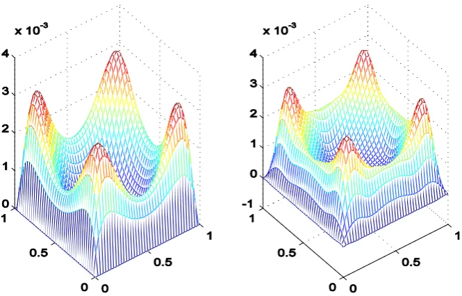
[image:6.595.83.519.298.472.2]

Fig. 3. An exact solution versus fictitious values (left) and absolute of the difference between an exact solution and an approximate solution (right) of Example 4.1 using regular scattered nodes.

Table 1. Maximum relative errors and root mean square relative errors using linear basis of Example 4.1.

N εmax εrms

16 0.087161168170710 0.043580584085307

25 0.050358497618669 0.030113754701725

36 0.032361053913413 0.021484740518138

49 0.023035676208513 0.016387047401505

64 0.017143934984936 0.012673300080537

81 0.013492037450895 0.010323479185026

100 0.010879139865142 0.008417391483891

121 0.002336287440439 0.001632271994812

144 0.002167180993382 0.001403315986505

169 0.002084551491908 0.001344174231217

[image:6.595.110.487.533.690.2]

[image:7.595.68.496.108.497.2]

Table 2. Maximum relative errors and root mean square relative errors using quadratic basis of Example 4.1.

N εmax εrms

16 0.050623969866327 0.045828966736731

25 0.031908920567838 0.030352930169516

36 0.022606591744903 0.021037079186475

49 0.016482360093915 0.015987485213218

64 0.012806666014302 0.012121872348316

81 0.010070455041601 0.009807325440163

100 0.001516655001101 0.007871532231840

121 0.001257510217670 0.001107414913633

144 0.001135033256359 0.000889648047242

169 0.000986069196989 0.000813703288717

[image:7.595.71.537.545.742.2]

196 0.000916579334735 0.000683806526348

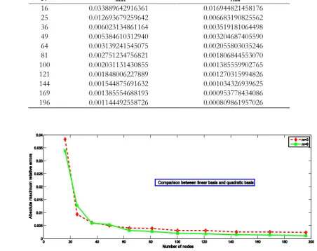
Fig. 4. Maximum relative errors as a function of nodal points of Example 4.1.

According to Fig. 4 and Fig. 5, it can be seen that both errors have the same results no matter what linear or quadratic polynomial bases are used for nodal shape construction; moreover, increasing a number of nodal points can be decreased maximum relative errors and root mean square relative errors. It can be observed that the agreements between numerical and exact solutions are quite excellent, and the convergence is very good as well as computational efficiency.

4.2. Uniformly Distributed Load on a Simply Supported Square Plate

An exact solution in term of deflection is given by

 



 



 

2 2

6

2 2 2

16 1

( , ) sin sin , , 1,3,5,...,

( )

m n

q m x n y

w x y m n

m n

D a b

mn

a b

(23)

For numerical implementation of Example 4.2, a characteristic length that is related to the nodal spacing in the local domain of the point of interest must be reconsidered and changed to include small number of nodes in order to avoid the singular of moment matrix leading open-end research for criteria which has been satisfied in terms of compact support. Similarly, Fig. 6 shows the fictitious values w versus exact solution and absolute value of the difference between exact solution and approximate solution while tabular errors using linear basis and quadratic basis for nodal shape construction of Example 4.2 are shown in Table 3 and Table 4, respectively. According to both tables, these results show the convergence of this method by increasing the number of nodal points. In addition, illustratively, the results of absolute maximum relative errors and root mean square relative errors are plotted as a function of nodal points are shown in Fig. 7 and Fig. 8, respectively. In addition, the numerical result measured by absolute maximum relative errors and root mean square relative errors, which are less than 0.2 percent, are acceptable when choosing the number of nodal points more than 121.

[image:8.595.72.529.423.581.2]

[image:9.595.112.484.103.272.2]

Table 3. Maximum relative errors and root mean square relative errors using linear basis of Example 4.2.

N εmax εrms

16 0.038353872791667 0.019176936395791

25 0.009383263980405 0.005072878779049

36 0.006155993321604 0.003613485915918

49 0.005060284332652 0.003103139960949

64 0.004041083163217 0.002483841146979

81 0.003953994544401 0.002298035513256

100 0.003141485983959 0.001923332980279

121 0.003126004082891 0.001816127366002

144 0.002571966761904 0.001574562565915

169 0.002578677958295 0.001509485998412

[image:9.595.109.483.320.490.2]

196 0.002387434960509 0.001347164501525

Table 4. Maximum relative errors and root mean square relative errors using quadratic basis of Example 4.2.

N εmax εrms

16 0.033889642916361 0.016944821458176

25 0.012693679259642 0.006683190825562

36 0.006023134861164 0.003519181064498

49 0.005384610312940 0.003204687405590

64 0.003139241545075 0.002055803035246

81 0.002751234756821 0.001806844553070

100 0.002031131430855 0.001385559902765

121 0.001848006227889 0.001270315994826

144 0.001544875691632 0.001034326939625

169 0.001385554688193 0.000953778434086

196 0.001144492558726 0.000809861957026

[image:9.595.70.523.332.690.2]

[image:10.595.70.523.83.249.2]

Fig. 8. Maximum relative errors as a function of nodal points of Example 4.2.

4.3. Hydrostatic Load on a Simply Supported Rectangular Plate

An exact solution in term of deflection is given by

 









 



 

2 1 2

6

2 2 2

8 ( 1)

( , ) sin sin , , 1,2,3,...

( )

m

m n

q m x n y

w x y m n

m n

D a b

mn

a b

(24)

Unlike previous numerical examples, we construct MK nodal shape function by using unconventional nodal arrangement for numerical result perspectives. 11x11 typical unconventional nodal arrangement is chosen for constructing MK nodal shape function with using linear and quadratic polynomial basis. Illustratively, the fictitious values and exact solution is shown corresponding linear, quadratic and cubic polynomial basis in Fig. 9 and Fig. 10, respectively. Similarly, these figures show that their exact solutions versus fictitious values have the same outcome.

[image:10.595.172.425.484.673.2]

[image:11.595.172.425.79.271.2]

Fig. 10. An exact solution versus fictitious values of Example 4.3 using an 11x11unconventional nodal arrangement with quadratic polynomial basis

4.4. Irregular Domain: A Hollow Square Plate

An analytical solution in term of deflection may be given by

 

_ 1 2 1 2 1 2_

2

3 2 5

( , ) ( ) ( ) ( ) sin( )sin( )

w x y x y x y

(25)

Firstly, before constructing moving Kriging nodal shape function, a 152-nodal-point proper arrangement corresponding to problem geometry, a hollow plate, which shown in Fig. 11 is conducted. Secondly, choosing linear and quadratic polynomial bases based on MK with this nodal arrangement, we obtain the shape function. Finally, computing numerically integrands according to discretization section we obtain trial function, namely, an approximate solution of plate deflection

Fig. 11. A hollow-plate nodal arrangement.

[image:11.595.148.424.478.689.2]

[image:12.595.95.485.99.279.2]

Fig. 12. A comparison of an analytical solution profile (left) and an approximate solution profile (right) of Example 4.4. using linear polynomial basis nodal shape function.

Fig. 13. A comparison of an analytical solution profile (left) and an approximate solution profile (right) of Example 4.4. using linear polynomial basis nodal shape function.

The maximum absolute value of the difference between an exact solution and an approximate solution is approximately 0.001376 while the maximum of root mean square value of the difference between an exact solution and an approximate solution is approximately 0.000722 when using either linear polynomial basis or quadratic polynomial basis.

[image:12.595.137.470.354.567.2]

between numerical and analytical results are quite excellent, and the convergence is very good as well as computational efficiency. Increasing the number of nodal points is a one of crucial factor for providing the convergence of the solution as well as an appropriate choice of nodal shape construction.

5.

Conclusions

An alternative meshless method, a specific numerical method, has been presented for solving thin plates problems subjected to various loads. Moving Kriging interpolation method is considered for constructing nodal shape functions as well as two field variables scheme is proposed by decomposing the biharmonic equation into a coupled of Poisson’s equations; furthermore, two-field variables local weak forms using Heaviside function enable us to tackle the complicated conventional local weak form of the biharmonic equation in the sense of numerical quadrature occurring in conventional local weak form as well as impose straightforward the simply supported boundary condition, For these reasons, computer literacy is also conducted systematically in the sense of easiness and robustness and its implementation is also acceptable as well. Comparing between exact solution and approximate solution for all examples, numerical results show that using the quadratic polynomial or linear basis gives quite accurate numerical results. Using moving krigking method for constructing nodal shape function, it can be concluded that there are no the difference between absolute maximum relative error and root mean square relative error results when using many more the number of nodal points.

References

[1] R. A. Gingold, and J. J. Moraghan, “Smooth particle hydrodynamics: Theory and applications to non spherical stars,” Monthly Notices of the Royal Astronomical Society, vol. 181, no. 2, pp. 375−389, 1977. [2] P. Krysl, and T. Belytschko, “Analysis of thin plates by the element-free Galerkin method,” Comput.

Mechanics, vol. 17, pp. 26−35, 1995.

[3] G. Liu, “Moving Kriging interpolation and elememt-free Galerkin method,” Int. J. Numer. Methods Eng., vol. 56, pp. 1−11, 2003.

[4] S. N. Atluri, and T. Zhu, “A new meshless local Petrov-Galerkin (MLPG) approach in computational mechanics,” Computational Mechanics, Vol. 22, pp. 117−127, 1998.

[5] S. N. Atluri, and T. Zhu, “A new meshless local Petrov-Galerkin (MLPG) approach to nonlinear problem in computer modeling and simulation,” Computer Modeling and Simulation in Engineering, vol. 3, pp. 187−196, 1998.

[6] S. N. Atluri, H. G. Kim, and J. Y. Cho, “A critical assessment of the truly meshless local Petrov-Galerkin (MLPG), and local boundary integral equation (LBIE) methods,” Computational Mechanics, vol. 24, pp. 348−372, 1999.

[7] S. N. Atluri, and S. Shen, “The meshless local Petrov-Galerkin (MLPG) method: A simple and less-costly alternative to the finite element and boundary element methods,” Computer Modeling in Engineering & Sciences, vol. 3, no. 1, pp. 11−51, 2002.

[8] S. N. Atluri, and S. Shen, The Meshless Local Petrov-Galerkin (MLPG) Method, Tech Science Press, Encino, pp. 11−51, 2002.

[9] S. N. Atluri, and T. Zhu, “The meshless local Petrov-Galerkin (MLPG) approach for solving problems in elasto-statics,” Computational Mechanics, vol. 25, pp. 169−179, 2000.

[10] S. Y. Long, and S. N. Atluri, “A meshfree local Petrov-Galerkin method for solving the bending problem of a thin plate,” CMES-Comput. Model. Eng. Sci., vol.3, pp. 53−63, 2002.

[11] V. Sladek, J. Sladek, and L. Sator, “Physical decomposition of thin plate bending problems and their by mesh-free methods,” Eng. Anal. Boundary Elem., vol. 37, pp. 348−365, 2013.

[12] S. Kaewumpai, S. Tangmanee, and A. Luadsong, “A meshless method based on radial point interpolation with two field variables for solving thin plate problems,” Far East Journal of Mathematical Sciences, vol. 85, no. 1, pp. 67−85, 2014.