Enhanced tracking and recognition of moving objects by reasoning about spatio-temporal continuity.

This is a repository copy of Enhanced tracking and recognition of moving objects by reasoning about spatio-temporal continuity..

White Rose Research Online URL for this paper: http://eprints.whiterose.ac.uk/7824/

Article:

Bennett, B., Magee, D.R. orcid.org/0000-0003-2170-3103, Cohn, AG

orcid.org/0000-0002-7652-8907 et al. (1 more author) (2008) Enhanced tracking and recognition of moving objects by reasoning about spatio-temporal continuity. Image & Vision Computing, 26 (1). pp. 67-81. ISSN 0262-8856

https://doi.org/10.1016/j.imavis.2005.08.012

Reuse See Attached Takedown

If you consider content in White Rose Research Online to be in breach of UK law, please notify us by

Enhanced tracking and recognition

of moving objects by reasoning about

spatio-temporal continuity

Brandon Bennett

, Derek Magee

, Anthony Cohn

and

David Hogg

a_{School of Computing, University of Leeds, Leeds, LS2 9JT,UK}

Abstract

A framework for the logical and statistical analysis and annotation of dynamic scenes containing occlusion and other uncertainties is presented. This framework consists of three elements; an object tracker module, an object recognition/classification module and a logical consistency, ambiguity and error reasoning engine. The prin-ciple behind the object tracker and object recognition modules is to reduce error by increasing ambiguity (by merging objects in close proximity and presenting multiple hypotheses). The reasoning engine deals with error, ambiguity and occlusion in a unified framework to produce a hypothesis that satisfies fundamental constraints on the spatio-temporal continuity of objects. Our algorithm finds a globally con-sistent model of an extended video sequence that is maximally supported by a voting function based on the output of a statistical classifier. The system results in an annotation that is significantly more accurate than what would be obtained by frame-by-frame evaluation of the classifier output. The framework has been im-plemented and applied successfully to the analysis of team sports with a single camera.

Key words: Visual Surveillance, Spatial Reasoning, Temporal Reasoning, Resolving Ambiguity, Continuity

1 Introduction

systems based on object tracking. In this paper we propose a framework for enhancing the imperfect output of an object tracker by enforcing principles of logical consistency and spatio-temporal continuity of physical objects. This results in a scene annotation that is far more accurate than the raw output from the tracker.

Our tracker processes a video recording of a dynamic situation, taken with a single fixed camera (i.e. a sequence of 2D images). Using statistical techniques, the tracker detects and classifies moving objects in the scene. The tracking and recognition systems explicitly model the possibility of ambiguity and error by assigning probabilities for the presence of objects within bounding boxes in each video frame. However, the tracker output is unreliable in that: a) the object detected with the highest probability may not actually be present in the box; b) there may be multiple overlapping or occluding objects within any box, and the tracker output does not tell us how many objects are present.

This imperfect tracker output output is passed to a reasoning engine which constructs a ranked set of possible labellings for the whole video sequence, that are consistent with the requirements of object continuity. The final output is then a globally consistent spatio-temporal description of the scene which is maximally supported by probabilistic information given by the classifiers.

A number of researchers have attempted to deal with object occlusion (and the resultant tracking problems) by attempting to track through occlusion. This can involve reasoning about object ordering along the camera optical axis, either using ground-plane information [1–3] or simply reasoning about relative spatial ordering [4]. 3D [3] or 2D (planar) [1] object models may be used with a known camera-to-ground-plane transformation to identify occlusion for a given set of object configurations. This can then be used to exclude subsets of image information from the model fitting process. This works well for ‘hypothesise-and-test’ type tracking (e.g. [2]). However, complete occlusion leads to zero information from the image, and weak constraints on object position/configuration. [5] takes a conservative approach of not tracking in uncertain situations, such as object occlusion. The ends of broken tracks are then joined based on spatio-temporal similarity measure.

Another approach has been to use multiple cameras in an attempt to circum-vent the occlusion problem. In [6] multiple football players are tracked using eight cameras. Each view is tracked separately and overlapping/occluding ob-jects are associated with the same blob (as in our system). Each blob from each camera is projected to the ground-plane (using a camera calibration), and associated with one, or more, players using a “closed-world” assumption, and a stochastic constraint optimisation procedure.

posi-tion of occluded objects [7,8], under the assumpposi-tion of known dynamics (e.g. linear motion), when no visual information is available. In [9] the authors use both motion models and 2D dynamic appearance models to track through oc-clusion. This work is interesting as it is a composite of a moving region (‘blob’) segmentation/extraction algorithm (that has no explicit notion of occlusion), and a model based tracker, that can track through partial and (short term) complete occlusion using motion and appearance models.

The success (or otherwise) of tracking through occlusion with motion and appearance models depends on a number of factors: the degree to which the models accurately model object dynamics and appearance, the time over which the occlusion occurs, the complexity of object behaviour during occlusion, the degree to which objects are occluded (partially or completely), and the similarity (or otherwise) of the occluding objects. Our proposed method (see later) is independent of all these factors (except object similarity). Multiple cameras have also been used to bypass the occlusion problem [10,11]. However, this is not always possible or practicable, and it is not necessarily a complete solution.

tempo-ral consistency rules are used to prune transient objects resulting from noise. None of these systems performs more than frame-by-frame reasoning or allows for the possibility of error in the underlying low-level tracking and recognition algorithms. Our system performs long-term reasoning about object-blob asso-ciations over extended sequences of frames. By maintaining spatio-temporal consistency over sequences, many local imperfections and ambiguities in the low-level data are eliminated.

Our system is based on ‘blob tracking’ and object classification methods. Much prior work has been presented in these areas. ‘Blob tracking’ may be described as tracking with a weak object model. This has the advantage that trackers based on this approach (e.g. [16,17,9,18]) are able to track a wide range of objects. Such trackers are often based on background modelling methods (e.g. [16,9,19]), which are used to extract foreground regions that are associated over time. The disadvantage is a lower grade of information is obtained; typically only position, scale and 2D shape are extracted. In contrast, model-based trackers may extract pose [3], posture [20] or identity information [21], for a particular (known) class of objects objects only. The acquisition of good models for model based tracking is also a non-trivial problem.

The extraction of a wider range of parameters from ‘blob tracker’ output may be seen as a separate post-processing operation. In [22] neural networks are used to classify vehicle type (small, medium, or large) based on edge informa-tion in the region around an object detecinforma-tion. In [23] a k-nearest neighbours classifier based on vector quantisation (similar to that used in our work) is used on various simple object features (height/width ratio, area, etc.) to clas-sify tracked objects as pedestrian or bicycle. In [24] the output of a blob tracker is classified in an unsupervised manner into various categories (representing colour, and texture etc.). From this temporal protocols are learnt. In [12] his-tograms of foreground pixel colour are used to parameterise appearance and recognise individuals at a later time, using histogram intersection. We also use the colour histogram approach. However, any of the classification approaches described (or others) could be used equally well within our framework. Classi-fication using colour histograms is simply used as an example to demonstrate the power of the reasoning framework presented. Using more complex classi-fication methods would obviously improve the initial classiclassi-fication. However, we argue that no classification method is 100% accurate in unconstrained sce-narios and there is always a potential benefit from the type of spatio-temporal reasoning presented in this paper.

advocated in a number of computer vision contexts before (e.g. [33–37]). Of particular relevance is work on spatial change [30], and continuity networks (aka conceptual neighbourhoods), which encode those transitions between re-lations that are consistent with an underlying notion of continuous change [28]. Such knowledge can be used for example to perform qualitative simu-lations [38] or to filter video input for consistency [33]. However we are not aware of any work in this area specifically addressing the focus of this article: tracking and recognition of moving objects using explicit symbolic qualitative notions of continuity.

2 An Architecture for Tracking and Recognition with Error Cor-rection based on Consistency Reasoning

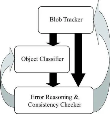
Our proposed architecture consists of three parts: i) a modified ‘blob tracker’, ii) an object recognition/classification system, and iii) an error reasoning and consistency checking module. The relationship between these components is illustrated in figure 1.

Fig. 1. An Architecture for Robust Scene Analysis

3 The Blob Tracker

Much effort has been put into visual object tracking methods over the last two decades, and a number of methods have been developed that are robust under certain constraining conditions. These constraints are usually on the type of motion possible (e.g. Kalman filter based trackers such as [7] assume approxi-mately constant velocity), on the total number of objects possible and on the types of multiple object occlusions possible. There is little evidence of any object tracking system that will work in completely unconstrained scenarios such as crowd scenes (e.g. in an crowded airport terminal), or for team sports surveillance (e.g. football, rugby or basketball). A popular solution to this is to present tracking results as a probability density over a space of possible model configurations, as for example the CONDENSATION algorithm of Is-ard and Blake [2]. This works well for propagating short-term (frame to frame) configuration information; however these densities are usually represented as approximations to the true density, and long term configuration information is not preserved. This is compounded by the fact that many high level sys-tems that use the output of such object trackers require as their input a single track result (for example [7,39]). In such cases the maximum a-priori proba-bility configuration (or similar) is usually taken and the information present in the densities is lost (we do not encourage such an approach!).

In contrast, more traditional single hypothesis (e.g. Kalman filter based) object trackers are now becoming popular again for multiple object tracking due to their lower computational cost and demonstrable robustness (the system of Stauffer and Grimson [16,17] has been running on-line for a number of years with a very low error rate). These benefits are of course at the expense of detail in the tracker output (such as object identity or pose). However, in many applications this detail is not required, or can be obtained from a separate module. The object tracker used in this paper is an extension of the car tracker of Magee [18], which in turn is based on the work of Stauffer and Grimson [16,17]. The tracker is operates in the 2D image plane (as opposed to the 2D calibrated ground-plane of the original work [18]). The principle behind these trackers is illustrated in figure 2.

Fig. 2. Schematic of Blob Tracker Operation

This technique reduces to near zero the occurrence of tracker errors such as lost/additional objects in our chosen example domain. The remaining errors may be eliminated by more traditional techniques such as ignoring transient objects (i.e. objects present only for a very short period of time). An example of the tracker output for a simple basketball sequence is given in figure 3.

a) b) c) d)

e) f) g) h)

Fig. 3. Example Output Sequence from Blob Tracker

containing the blob (typically 3 standard deviations). Assuming a Gaussian distribution of blob pixel locations along 1D axes, this means (for a threshold of 3 standard deviations) statistically >99% of blob foreground pixels should lie within this bounding box.1 A similar confidence for the bounding box could not be derived from a simple per-frame bounding box of pixels classified as foreground associated with the blob, as there is a non-zero probability of a mis-classification of a pixel as foreground/background. The ‘statistical’ bounding box described is used in the error reasoning and consistency checking module (section 5).

4 Object Classification

As noted above, we cannot expect an object recognition/classification sys-tem to have 100% accuracy except under very restricted operating conditions. However, our higher-level processing (see section 5) is designed to cope with imperfect and ambiguous input. Indeed, the power of the reasoning system can only be fully appreciated when there is significant error in the classifier output.

We have implemented a system that combines a number of simple exemplar-based classifiers. Positional and foreground segmentation information provided by the tracker is used to determine a feature description of each object tracked. Our classification module has very low computational cost and so can be incor-porated into an on-line system. (Currently the reasoner operates as an off-line post-processor for the tracker/classifier output. The possibility of implement-ing an on-line reasoner will be discussed in Section 5.5.)

A colour histogram using the UV colour-space is formed for each object tracked, using the colour values of the foreground pixels identified as belonging to that object by the object tracker. The UV colour-space is a 2D truncation of the 3D YUV colourspace that separates colour (UV) and intensity (Y) into separate channels2_{. We discard the intensity channel to give a degree of}

light-ing invariance. A trainlight-ing video sequence is automatically tracked (uslight-ing the object tracker), and the objects identified hand labelled with their identity (at approximately 1 second intervals). Around 50 examples of each object are used. The resultant set of histograms is clustered, using the K-means clus-tering algorithm, to give a set of exemplar histograms (corresponding to the cluster means). Each cluster is assigned an object label based on the identity

1 _{In practice, the proportion of blob pixels within the bounding box is 100% for}

most frames, due to the finite number of pixels associated with each blob, and the actual distribution having a shorter tail than a Gaussian.

of the majority of training examples in that cluster. The number of clusters is selected such that each cluster contains at least 99% examples of a single iden-tity, and there is at least one cluster relating to each possible identity. These labelled exemplars are used (on unseen sequences) as an object classifying model. The advantage of the exemplar approach is that new objects/classes can be added to the system easily without a full re-training stage. This is near essential if training is to be performed on-line as new objects appear (although we currently work with a ‘closed-world’ offline scenario where all possible objects are known a-priori).

To apply our exemplar-based model to an unseen tracked object, a YU colour histogram is formed for the unseen object in exactly the same way as for the training examples. A model exemplar histogram represents the probability dis-tribution over colour for a single pixel (P(colour|modeln)). A data histogram represents the normalised frequency distribution of colour values. Therefore, to calculate the probability of the novel data observed with respect to a single exemplar (P(observation|modeln)) it is simply a matter of representing the two histograms as matrices and calculating the correlation between these two matrices (equation 1).

P(observation|modeln) =

Nbins X

b=1

DbMb (1)

Where:

Db = Binb of the data histogram

Mb = Binb of the model histogram

Nbins = The number of bins in the histograms

Using Bayes law:

P(modeln|observation) =P(observation|modeln)P(modeln)

P(observation) (2)

=P(modeln)∗

Nbins X

b=1

DbMb

Pb (3)

Where:

Pb = Bin b of the mean histogram over all training examples

P(modeln) = The a-priori probability of the exemplar.3

3 _{We use 1/no of exemplars, as each exemplar represents approximately the same}

To obtain the probability that an observation is of a particular identity,

P(identitym|observation), the maximum value ofP(modeln|observation) over all exemplars relating to that identity is taken. Taking the maximum value is appropriate as the different exemplars relating to a particular identity gener-ally relate to different object configurations or viewpoints. As such, exemplars relating to object configurations or viewpoints other than the actual ones pro-vide little information. These probabilities (along with the object locations and sizes from the object tracker) are passed on to the reasoning engine (de-scribed in section 5).

4.1 Box Classifier Output

Once the probabilities of each object being in each box have been computed, each frame of input is represented by a data structure encoding both the tracker box geometries and the associated object probabilities. The represen-tation is illustrated in Figure 4. A sequence of these structures will form the input to the reasoning module of our system.

frame(500, 2, %% Frame count, Number of boxes %% List of box data objects

[ box( 7, 6, %% ID tag, Parent ID

[afro, derek, ball], %% Objects detected

[0.761138, 0.130362, 0.0253883], %% Respective robabilities [[283.4,133.6],[75.9,121.2]] ), %% Box geometry

box( 8, 6,

[afro, derek, ball], [1, 0.13897, 0.0253883], [[95.9,133.0],[74.2,125.7]]) ]).

Fig. 4. Tracker/classifier data sent to Prolog reasoning engine

5 Ensuring Spatio-Temporal Continuity

C1) exclusivity — an object cannot be in more than one place at the same time;

C2) continuity — an object’s movement must be continuous (i.e. it cannot instantaneously ‘jump’ from one place to another).

In the output given by any statistical classifier, it is quite possible that an object is detected to a high degree of probability in two locations that are widely separated. This kind of error is fairly easy to eliminate on a frame by frame basis. We can consider all possible assignments of different objects to the tracked boxes in each frame and chose the combination that maximises the summed probabilities of object to box correspondences.4

The continuity of an object’s position over time is much more difficult to model; and considerable problems arise in relating continuity constraints to tracker output. The main problem is that of occlusion: if an object moves behind another it is no longer detectable by the tracker; so, under a naive in-terpretation of the tracker and recognition system outputs, objects will appear to be discontinuous.

As well as ensuring spatio-temporal constraints are respected, we also want to find an object labelling which is maximally supported by the frame-by-frame tracker output and the probabilistic output of the object recogniser for each tracked box. However, the recognition system was trained to identify single objects, whereas in tracking a dynamic scene there will often be several objects in a box. This means there is no completely principled way to interpret the output figures from the recogniser. Nevertheless, it seems reasonable to assume that although there is a large amount of error and uncertainty in the low-level output, it does give a significant indication of what objects may be present. We shall explain below exactly how our system converts low-level statistics into a metric of the likelihood of any given set of objects being in a box.

Local continuity information is provided by the low-level tracker module. The tracker output assigns to each blob’s bounding box an identification tag (a number), which is maintained over successive frames. For newly split or merged boxes new tags are assigned but the tag of their parent box in the previous frame is also recorded. Thus each box is associated with a set ofchild boxes in the next frame. Conversely each box can be associated with a set of itsparent

boxes in the previous frame. The parent/child relation determines a directed graph structure over the set of boxes, which we call a ‘box continuity graph’. Such a graph is illustrated in figure 5. Our algorithm depends on the structure of this graph, which will be examined in more detail later.

4 _{This assumes that the classifier is capable of identifying unique objects (such}

Fig. 5. Tracker output expressed as a ‘box continuity’ graph

The continuity-based reasoning algorithm involves a somewhat complex re-structuring of the available information. To describe its operation we start by formally specifying the information associated with a tracked box and the output of the classifier when applied to that box. Formally, a tracker box b

can be represented by a tuple,

hf,geom,pa,ch,Classi ,

where f is the frame number, geom is the box geometry, pa is the set of its parent boxes (in the framef−1), chis the set of its child boxes (in the frame

f+1) andClassrepresents the statistical output of the object classifier applied to this box. Frame numbers are elements of a continuous subset of the non-negative integers with the usual ordering. The initial frame will be denotedf0.

For convenience we introduce the functions f(b), geom(b), pa(b), ch(b) and

Class(b) to refer to the corresponding information associated with boxb. The set of all boxes in the tracker/recogniser output will be denoted by BOXES_.

From the point of view of object continuity, the parent and child boxes of a given box can be regarded respectively as ‘sources’ and ‘sinks’ of that box. The occupants of a box must have come from its parent boxes and must go to its child boxes. Assuming no objects enter or leave a scene, each box is associated with at least one source box in the previous frame and one sink box in the next frame. However, where two or more boxes become merged, the merged box will have more than one source; and, when a box is split, it will have two or more sinks. We do also allow objects to enter or leave the scene, so there may be some boxes with no source or no sink.5

5 _{Such boxes would typically occur at one or other side of the scene, but in the}

Within the box continuity graph are chains of boxes linked by a unique source-sink relationship (see Figure 5). Each of these corresponds to the ‘history’ of a tracker box between splitting and merger events. If the tracker were perfectly accurate, the objects occupying any box would be constant along any of these linear sub-graphs. Hence, assuming such perfect accuracy, one can enforce a localised continuity constraint by simply requiring that box labellings are constant along such sub-graphs. However, as we have already noted, where there is some overlap between boxes, objects may sometimes transfer between boxes. This possibility will be considered in the next section.

To model spatio-temporal continuity is useful to introduce an abstract data object which we call a spatio-temporal box (ST-box for short). ST-boxes will normally be denoted by symbols Si. In the tracker output, an ST-box cor-responds to a temporally continuous sequence of boxes which have the same tag. In terms of the ch function, this is a maximal sequence [b1, . . . , bn] such

that for eachi in the range 1≤i≤n−1 we have ch(bi) ={bi+1}.6

It is convenient to represent an ST-box as an ordered set S indexed by frame numbers in the range s(S). . .e(S), where the functionss(S) ande(S) denote respectively the start and end frames of the period over whichSexists. We also define the partial function box-at(f, S) to denote the box b ∈S whose frame number isf. This function is only defined forf in the ranges(S)≤f ≤e(S). Clearly each boxb∈BOXES_{is a member of a unique ST-box which we denote}

by st(b). The set ST-BOXES _{={S | (∃b ∈} BOXES_{)[st(b) = S] } is the set of}

all ST-boxes.

5.1 Coarse Object Grouping with ‘Envelopes’

Although the tracker output enables us to derive a graph representing tempo-ral continuity between tracked boxes, this structure is only indirectly related to the trajectories of actual moving objects in the scene. There are several issues that complicate the relationship between tracker boxes and objects. Firstly, there is the basic problem caused by proximal and/or occluding objects, which means that a box may be occupied by several objects. This is compounded by the possibility that objects sometimes transfer between tracker boxes without themselves being independently tracked. This can occur because of occlusions among objects or because of limited resolution of the tracker (or a combination of the two). When a box containing more than one object is close to or overlaps another box, an object from the multiply occupied box can easily transfer to

6 _{This definition means that an ST-box may persist across a split or merger event.}

the neighbouring box without being detected. Conversely, undetected transfers are almost always between boxes whose geometries overlap.

A consideration of these problems led us to the idea that in order to get a more accurate identification of the locations and movements of closely grouped or occluding objects, we need to employ a representation in which the locations of objects are modelled at a coarser level than that of individual boxes. Hence, we introduced a higher level abstract data object that we call an envelope. Intuitively, we can regard an envelope as a maximal cluster of overlapping ST-boxes (this will shortly be defined more precisely). The concept of an envelope is illustrated diagrammatically in figure 6. Here, the shaded areas indicate the positions of boxes over a sequence of frames and thus correspond to ST-boxes. The dashed lines show the division of this structure into envelopes.

Fig. 6. Deriving Spatio-temporal Envelopes from Tracker Output

The definition of an envelope depends upon specifying an overlap relation between boxes, which we write formally as Overlap(b1, b2). Since, the boxes

To characterise what constitutes an envelope we first introduce the concept of aconstant-local-group spatio-temporal box orCLG-ST-box. This is a temporal sub-division of an ST-box, over which it is a member of a constant ‘local group’ of spatially overlapping ST-boxes. Thus it is part of the same cluster of ST-boxes throughout this period. Whereas the beginning and end frames of ST-boxes are determined by merger and splitting, the beginning and end frames of CLG-ST-boxes are determined by changes in the overlap relation between boxes. The division of ST-boxes into CLG-ST-boxes is indicated in figure 6. The divisions coincide with the temporal boundaries of the envelopes.

Local groups are sets of ST-boxes that are related by the transitive closure of the Overlap relation. This relation is written as Overlap∗(b1, b2).7 At

each frame over which it exists, any given ST-box stands in the Overlap∗

relation to a set of other ST-boxes, which is its local group at that frame. SinceOverlap∗ is reflexive, symmetric and transitive, at each frame the local groups form equivalence classes over the set of ST-boxes. Given an ST-box S

and a frame f (with s(S)≤f ≤e(S)), we can define the function

local-g(f, S) = {S′

|Overlaps∗(box-at(f, S),box-at(f, S′

))} .

A CLG-ST-box can now be defined as a subset of an ST-box corresponding to a maximal temporally continuous sequence of frames F = [fm, . . . , fn], such that for each fi ∈F, the function local-g(f, S) takes a constant value. Each ST-box determines a unique CLG-ST-box for each frame over which it exists. Hence we can define the function

clg-st(f, S) = {b∈S | local-g(f(b), S) = local-g(f, S)∧

¬∃f′_{[((f(b)< f}′ _{< f)∨(f < f}′ _{< f(b)))∧local-g(f}′_{, S)6=local-g(f, S)]} .}

The set of all CLG-ST-boxes is given by

CLG-ST-BOXES_{={C | (∃S∈}ST-BOXES_{)(∃f)[(s(S)≤f ≤e(S))∧}

clg-st(f, S) =C]}

As with ST-boxes, we use the functions s(C) and e(C) to refer respectively to the start and end frame of a CLG-ST-box, C. We also writest(C) to refer to the unique ST-box of which C is a sub-sequence.

Since CLG-ST-boxes participate in the same local group throughout their history, we can define the functionlocal-g(C), which does not require a frame argument:

local-g(C) = local-g(s(C),st(C)).

7 _{That is, Overlap}∗

(b1, bn) holds just in case there is some sequence of boxes

We can now define an envelope as a maximal set of overlapping CLG-ST-boxes. Any CLG-ST-box is a member of a unique envelope, given by

env(C) = {clg-st(s(C), S) |S ∈local-g(C)} .

For an envelopeE, the functionss(E) ande(E) denote the beginning and end frames of the envelope’s existence. By definition, all its constituent CLG-ST-boxes have the same beginning and end frames.

Each box in the tracker input is related to a unique envelope given by:

env(b) = env(clg-st(f(b),st(b)))

And the set of envelopes derived from the tracker input is given by:

ENVELOPES_{={E | (∃b∈}BOXES_{)[E =env(b)]}}

Later we shall want to refer to the set of envelopes that exist at a given frame. This is given by:

envs-at(f) ={E ∈ENVELOPES_{| s(E)≤f ≤e(E)}}

5.2 Enforcing Exclusivity and Continuity at the Envelope Level

Although envelopes give a coarser demarcation of object locations than do individual boxes, they provide a much more reliable basis for determining continuity. By definition, two different envelopes cannot spatially overlap (oth-erwise they would just be parts of a larger envelope). This means that there is an extremely low probability that an object can transfer between envelopes without being detected. Hence, our algorithm makes the assumption that the occupancy of an envelope is constant throughout its existence. The presence of object l in envelopeE will be formally specified by the relation Occ(l, E).

The exclusivity constraintC1, corresponds to the requirement that no object can occupy two distinct spatio-temporal envelopes that overlap in time.

C1) ∀E1E2lf [ (s(E1)≤f ≤e(E1))∧(s(E2)≤f ≤e(E2))∧

Occ(l, E1)∧Occ(l, E2))→(E1 =E2) ]

Functions returning parent and child sets for envelopes can be derived directly from the corresponding relations between tracker boxes:

pa(E) ={E′ _{| E}′ _6=E∧

(∃bb′ _∈BOXES

)[(env(b) =E)∧(env(b′

) =E′

)∧(b′ _∈pa

(b))]}

ch(E) = {E′ _{| E}′ _6=E∧

(∃bb′ _{∈BOXES)[(env(b) = E)∧(env(b}′_{) = E}′_)∧(b′ _∈ch(b))]}

Because we allow objects to enter and leave the scene we also need to keep track of off-scene objects. We do this by introducing virtual,off-scene envelopes

to our model. We could have different sets of off-scene envelopes for different entry/exit points but in the current implementation we assume there is only one off scene location. Transfer to and from off-scene envelopes can only occur when a tracker box is either created or disappears.

Off-scene envelopes do not have any spatial structure; so we identify them simply with a frame pair hfb, fei representing the beginning and end frames of their existence. The limiting frames of off-scene envelopes are defined as follows:

B-OFFENV_{={f | (∃E ∈}ENVELOPES_{)[ ((pa(E) =∅)∧(f =s(E)))∨}

((ch(E) = ∅)∧(f =s(E) + 1)) ] }

E-OFFENV_{={f | (∃E ∈}ENVELOPES_{)[ ((ch(E) = ∅)∧(f =e(E)))∨}

((pa(E) = ∅)∧(f =s(E)−1)) ] }

So the setOS-ENVELOPES _{contains all beginning/end frame pairs that have}

no other beginning or end frames occurring between them:

OS-ENVELOPES_{={hfb, fei |fb ∈}B-OFFENV_{∧fe ∈}E-OFFENV_∧

¬∃(f ∈(B-OFFENV_∪E-OFFENV_{)[(f > fb)∧(f < fe)] }}

The set including both on-scene and off-scene envelopes will be denoted by

ENVELOPES+₌ENVELOPES_∪OS-ENVELOPES_{. The predicateOS(E) holds}

just in caseE is an off-scene envelope.

In order to define the continuity relation between envelopes, it is convenient to first define a successor relation Suc(E1, E2), which holds when the end of E1 is at the frame immediately before the beginning of E2:

Suc(E1, E2) ≡def ((e(E1) + 1) =s(E2))

We can now define the relationSource-Sink(E1, E2), meaning that envelope E1 is a source for the objects in envelope E2. The following formula handles

Source-Sink(E1, E2) ≡def ((E1 6=E2) ∧

[ ∃b1b2[b1 ∈pa(b2)∧env(b1) =E1∧env(b2) = E2]

∨ (OS(E1)∧(pa(E2) =∅)∧Suc(E1, E2))

∨ (OS(E2)∧(ch(E1) =∅)∧Suc(E1, E2))

∨ (OS(E1)∧OS(E2)∧Suc(E1, E2)) ] )

In terms of this relation, the continuity constraint C2, as applied at the en-velope level, is represented by

C2) Occ(l, E1)→ ∃E2[Source-Sink(E1, E2)∧Occ(l, E2)] ∧

Occ(l, E2)→ ∃E1[Source-Sink(E1, E2)∧Occ(l, E1)]∧

Source-Sink(E1, E2)→ ∃l[Occ(l, E1)∧Occ(l, E2)]

Our algorithm will generate possible assignments of object labels to envelopes that satisfy both C1 and C2. It will then choose the one that we consider ‘best supported’ by the classifier outputs.

5.3 Observational Likelihood of Box and Envelope Occupancy

There is a finite set of potential explanations for the output presented by the blob tracker and object classifier that are consistent with the continuity constraints described in the previous section. But the number of possible ex-planations is extremely large even in simple scenarios. A metric is required to rank these based on the symbolic and probabilistic output of these lower level processes.

As described above, the low-level classifier computes probabilities based on a Bayesian combination of learnt binary colour-histogram classifiers. Applied to a box b the output takes the form

Class(b) ={hl1, p1i, . . . ,hln, pni} ,

where pi is the probability of li being a correct label for the object(s) in box b. The set of all labels known to the classifier will be denoted LABELS_.

Each statistic is an independently computed probability based on the assump-tion that there is only one object in the box. Thus, the figures are not nor-malised and cannot be reliably applied to cases where there is more than one object in a box. However, we assume that, even in multi-object cases, the fig-ures give an measure, albeit approximate and uncertain, of the likelihood of an object being in the box. Hence, we can regard the number pi directly as a ‘vote’ for the presence of object li in box b. We denote this vote value by

vote(l, b).

rather than individual boxes. Thus, we need to convert the votes for box occupancy into votes for an object being in a given envelope. There are a number of ways this could be done, none of which is really statistically valid. The function we have chosen is as follows: for an envelope E and an objectl, we compute for each CLG-ST-box C ∈E the sum of the box votes forl over all frames for which C exists. Thus

vote(l, C) = X

s(C)≤f≤e(C)

vote(l,box-at(f, C))

To get the vote for the object to be in an envelope we take the maximum of its votes for each CLG-ST-box in the envelope:

vote(l, E) = Max_{{ v | (∃C ∈E)∧vote(l, C) =v} .}

This would be reasonable on the assumption that the object stays in the same CLG-ST-box throughout its time within the envelope. This is not necessar-ily true, so the vote may be unreliable. Devising and evaluating more realistic voting functions is a subject of ongoing work. (Nevertheless, as will be seen be-low, our crude voting function is already a good enough metric to significantly enhance the reliability of recognition.)

In order to reduce the support value given to a label to the range [0. . .1], we compute the fractional vote forlwith respect to the total votes of all objects in the classifier domain{l1, . . . ,lN}. This is given by:

frac-vote(l, E) = _P vote(l, E)

i=1...Nvote(li, E) .

will be described in the next section). Because the votes computed this way all come out negative, we have found it more aesthetic to add a further +N, whereN is the maximum number of objects that may occur in the scene. This makes the votes positive, but is not really necessary because it is the relative scores of models we are interested in.

Another factor we wish to take into account is the duration over which an envelope persists. If we assume that the classifier outputs at each frame should have equal weight in determining what objects are present, then we should multiply the vote obtained by considering the labelling by the duration of the envelope. Hence, our aggregated voting function for multi-label envelopes is as follows:

vote({l₁, . . . ,ln}, E) = "

X

i=1...n

(frac-vote(E,li) !

−n+N

#

·dur(E),

where dur(E) = e(E)−s(E) + 1 is the duration of the envelope in frames.

For off screen envelopes, we take the vote for any set of labels to be 0.

5.4 Selecting the Best Hypothesis for an Extended Frame Sequence

The previous section defined a method for calculating a metric for ranking po-tential explanations of the output of the lower level systems. In principle, we could use this to evaluate all possible spatio-temporally consistent sequences of object labels. However, this would be infeasible for all but the shortest and simplest sequences. Whenever an envelope divides into two or more child envelopes, there are several possible assignments of the original envelopes oc-cupants to the newly created envelopes. Thus the number of possible solutions grows exponentially with time (as well as being an exponential function of the number of objects involved). However, by taking a dynamic programming [40] approach do the problem, the optimal solution can in fact be found by an algorithm whose complexity is linear in time. Thus, as long as the number of objects is relatively small, solutions for arbitrarily long sequences can be computed effectively.

An envelope labelling solution for a given tracker input assigns a set of labels to each envelope that satisfies the constraintsC1andC2. Our algorithm first computes the set of envelopes and theSource relation from the complete set of boxes output by the tracker.

it moves off the scene). We shall build a model by starting at the initial frame of the tracker output and progressing through each successive ECF. Since envelope occupancy remains constant between ECFs, this model actually de-termines a complete assignment to all envelopes at all frames. For any ECFf

(including the initial frame f0) the next ECF after f is denoted by necf(f).

When f is the last ECF in the input frame sequence we letnecf(f) = end_.

A spatio-temporally consistent assignment to all envelopes starting at or before some given ECFf will be called apartial model (up tof) and will be denoted Pi (where the optional i is a distinguishing index). lcf(Pi) denotes the last

change frame of envelopes assigned byPi. A partial modelP is identified with

a set {. . . ,hEi, Aii, . . .}, where Ai = {l1, . . . ,ln} ⊆ LABELS. The set must

contain an assignment for all envelopes starting at or before some ECF. The function ass(P, E) will denote the set of labels assigned by P to envelope E.

The requirement of spatio-temporal consistency of partial models means that the exclusivity and continuity constraintsC1andC2must be satisfied, where the occupancy relation Occ determined by a model P is given by Occ(l, E) iff l∈ass(P, E).

To compute a spatio-temporally consistent extension of a partial model, we need only know its assignments to the latest envelopes. Hence we define

last-ass(P) = {hEi, Aii | hEi, Aii ∈ass(P)∧s(Ei)≤lcf(P)≤e(Ei)} .

In order to formalise the notion of one partial model’s being an (immediate) extension of another, we define

Extends(P′

,P) ≡def ((P

′_\last-ass(P′

)) =P)

The set of all possible (spatio-temporally consistent) extensions of a partial model P is then given by

extensions(P) = {P′ _|

Extends(P′

,P)} .

extensions(P) is a key function of our algorithm. This function is straight-forward to compute. We first compute and store theSource-Sinkrelation for the tracker input, using the definitions given above. All we need to do is gen-erate all assignments to the envelopes in E′ _{= envs-at(necf(lcf(P))) which}

are consistent with the assignment to the envelopes in E =envs-at(lcf(P)). Using the definitions given above, it is straightforward to compute theSource

relation between envelopes in E and E′_.

of the partial model go to after the next ECF. The possible destinations are ‘sinks’ for these objects:

sinks(E) = { E′ _|

Source-Sink(E, E′_)}

To satisfy C2 we only need to ensure that for every E ∈ E, every label in

ass(P, E) is assigned to some envelope in sinks(E), and also at least one label in ass(P, E) is assigned to each E′ _{∈sinks(E). Moreover, it is easy to}

see that if the last assignment ofP satisfies the exclusivity condition C1then the assignment of any extension constructed in this way will also satisfy the

C1.

In order to choose which are most likely according to the object recognition software, we compute a vote measure for each model. The total support for a partial model is just the sum of the support for each of its envelope assign-ments:

vote(P) =X

{vi | hEi, Aii ∈ass(P)∧vote(Ai, Ei) = vi} .

In all but the simplest cases, we may have several different partial models that agree on their last assignment — i.e.last-ass(P1) =last-ass(P2). These,

rep-resent different assignment paths leading up to the same end state. Typically, one will have a higher vote support than the other, which gives an indication that one is the more likely of the two. In such a case we say that the more likely partial model subsumes the other:

Subsumes(P1,P2)↔((last-ass(P1) =last-ass(P2))∧vote(P1)>vote(P2))

Given a set M _{of partial models, we can ‘prune’ it to retain only the ‘best’}

models that lead up to any given final assignment.

prune-subs(M_{) = {P ∈}M_{| ¬∃(P}′ _∈M_)[Subsumes(P′_,P)]}

We initialise the set of partial models by considering all possible assignments of the domain objects to the initial envelopes, with the additional requirement that each envelope must be assigned a number of objects that is as least as many as the number of CLG-ST-boxes it contains. This initial partial model set will be denoted M_0.

f :=f0 M_:=M₀

while (f 6=end_{) {} M′ _:=∅

foreach (Pi ∈M) {

M′ _:=M′_{∪extensions(P) }} M_:=prune-subs(M′₎

f :=necf(f) }

We will not give a rigorous analysis of the complexity of our algorithm. How-ever, we can establish by informal argument that the model building algorithm (and hence also the selection of the optimal labelling) is essentially linear in the length of the video sequence and exponential in the number of objects involved in the scene.

The key observation is that there are a finite number of ways that a finite set of objects can be distributed among a finite set of envelopes. This number corresponds to the number of partitions into disjoint non-empty subsets of a set of given finite cardinality. It can be computed by a recursive algorithm and is bounded by an exponential. For example, in our main test data we track a scene with four moving objects (which can move on and off the screen). This means at any frame there are from 0 to 4 envelopes. Our pruning of low scoring models that are subsumed by better models with the same end state, means that number of partial models stored is limited to the number of distinct assignments that can be made to the end state of the sequence. For each of the cases of 0 to 4 envelopes, the number of assignments is respectively: 1, 15, 50, 60, 24. So the maximum number of models that must be stored is 60.8

At each cycle of the algorithm we extend each partial model to the next change frame. Again, although the number of possible extensions is exponential in the number of objects involved, for a fixed number of objects it is strictly bounded to a finite number of possibilities. Computing the new vote total for an extended envelope can be done in constant time since it depends only on the final assignment and the prior vote of the partial model being extended. Detecting the subsumptions among m newly extended models is O(m2_{), but}

is computationally trivial and here again m is bounded by a finite maximum depending on the number of objects in the scene.

8 _{The actual numbers of partial models stored will typically be considerably fewer}

These observations explain why for small numbers of objects, our algorithm performs very effectively. The crucial factor is our pruning policy means that the complexity becomes linear in the length of the frame sequence, even though we are finding the optimal of all possible models that are spatio-temporally consistent with that frame sequence. This pruning technique enables us to solve a highly intractable constraint problem by a method that can be seen as a kind of dynamic programming.

5.5 Off-Line Implementation of the Continuity Reasoner

The continuity reasoner has been implemented using the Prolog language (SICStus Prolog [41]). This allows easy creation and manipulation of the data structures required and a natural coding of the continuity reasoning algorithm. It currently runs in an ‘off-line’ mode — i.e. it processes a whole frame se-quence and then produces a globally consistent assignment for the complete sequence. This is a result of the way that we originally conceived the problem of achieving global consistency by enforcing constraints over the whole extent of a video sequence. We had thought that the best way of implementing this would be to start with a data model of the whole sequence and then use a general constraint solving technique to find consistent solutions. However, it eventually became clear that such solutions could be efficiently found by the sequential model building technique described in the previous section, which processes the input in the direction of time flow.

Because of the way it was developed, our current algorithm carries out a lot of pre-processing on the video sequence to build data-structures (representing the continuity graph of envelope objects) that are then used in the model building. However, it is now apparent that the whole algorithm could have been designed in an ‘on-line’ mode, where the envelope structure itself is built dynamically as the input frames are sequentially input. This would enable continual output of the best hypothesis for the current state of an ongoing video sequence. However, the dynamically generated best hypothesis up to a given frame would, in general, be less accurate than the hypothesis generated after processing the whole video sequence, because it would not take into account evidence from the object classifier relating to subsequent frames in the sequence.

6 Evaluation

The system was evaluated on approximately two and a half minutes of the basketball scene illustrated in figure 3. This scene consists of four objects (three players and a ball), variable numbers of which may be in the scene at any one time. The movie contains much interaction and occlusion that a conventional object tracker would find hard to track with a single camera. The movie is tracked and classified at 25fps and the results fed into the reasoning engine. The system was applied to a sequence of 2200 frames (88 seconds real time) and took approximately 5 minutes to generate all possible spatio-temporally consistent labellings.9 _{The model with the highest overall score}

was compared to a hand-annotated labelling which gives the ground truth at every 10th frame (plus some extra frames added at particularly dynamic parts of the video). Thus, over the length of the sequence a total of 612 tracked boxes were compared.

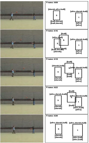
Figure 7 shows a typical output from the tracker, classifier and reasoner, for some illustrative frames of the video input (shown on the left of the figure). The frames show different stages of an event where a ball was passed from one player to another (from Derek Magee to Aphrodite Galata (Afro)). On the right we see the boxes detected by the tracker. The list shown above each box is the ranked list of labels output by the classifier. Here all labels detected with greater than a given probability threshold are given in decreasing order of probability (i.e. the leftmost label is the most probable). The list immediately below the box is the labelling assigned to this frame in the most likely globally consistent model generated by the reasoner. The list below this is the ground truth obtained by observing the video and hand labelling the tracker boxes. (The ordering of reasoner output and ground truth labels is just alphabetic.)

It is informative to look at the final frame (630), where the ball has been received by Afro. Here we see that the raw classifier output gives the list [afro,derek,ball] as ranked most likely labels for each of the boxes. This is clearly impossible in our scenario, since there is only one Aphrodite and she cannot be in two places at once. But the classifier output for this frame alone gives us no way to determine the best consistent labelling. Nevertheless, our reasoning algorithm, by considering continuity requirements over the duration of the sequence, has indeed found the correct labelling.

Looking at the output for the frames leading up to frame 630 gives an indica-tion of how the reasoner can work out a correct labelling from such inaccurate classifier output. Although the actual algorithm involves aggregating the clas-sifier’s probability values, a good intuition of how this works can be gained by

9 _{All experiments were carried out on a 500 MHz Pentium III; so real time}

thinking in terms of the probability-ranked labels shown above the boxes.

It will be seen that, at frame 609, Derek threw the ball towards Afro. In its processing of this frame, the classifier gives a higher probability for Afro rather than Derek to be in box 1, and also a higher probability for Derek rather than Afro to be in box 3. Thus, the correct labelling of the locations of Afro and Derek is better supported than any incorrect alternative (however there is nothing to suggest where or whether the ball is present). In frame 616, the ball is tracked as a new box, which overlaps with box 3. Boxes 3 and 5 are within the same envelope and the output shown gives the output from the reasoner on a per-envelope basis, with the labelling given under the lowest numbered box in the envelope.10 _{The high visibility of the ball in box 5}

increases its detected probability according to the classifier, and this supports its identification by the reasoner as being one of the objects in the envelope consisting of boxes 3 and 5. Moreover, because the reasoner enforces spatio-temporal continuity this also supports assignment of the ball label to box 3 at the earlier frame 609. In frame 619, box 5 no longer overlaps with box 3 and so is in an envelope on its own. Now it is well separated from other objects, the classifier correctly identifies the presence of the ball with high probability. Subsequently, in frames 622 and 630, box 5 overlaps and then merges with box 1. Thus, the detection of the ball in the earlier frames reinforces the assignment of the ball to box 1 in frame 630, in the maximally supported globally consistent model computed by the reasoning algorithm.

Comparing the output of the consistency reasoning algorithm with the raw output of the object recogniser is somewhat problematic, because the raw output does not give any indication of the number of objects that are in each box. The statistics given are just ranked probabilities of individual object being present. However, for purposes of comparison we must treat this data as somehow identifying a definite set of labels. To do this we use a rather rough heuristic: we say that the assignment includes any label which has the highest (or joint highest) probability of all those listed in the output, and also any other label identified with probability higher than 0.5. Figures computed from the resulting box-label assignments are given in the “Raw + HON” column of our tables of statistics (HON stands for heuristic occupancy number).

Another way of interpreting the raw output is to assume that the number of objects occupying each tracked box is somehow known by an independent procedure or oracle. Under this assumption one could use the ground-truth occupancy number, GON, to determine how many labels from the ranked la-bel list output by the classifier should be assigned to each box. The “Raw + GON” column shows these figures. Here, when evaluating a box which we know

10_{Subsequently, the per-envelope labellings are converted into a per-box labelling,}

(from human annotated ground-truth data) containsn objects, we take then

labels that are assigned the highest probabilities in the raw tracker/recogniser output.11 _{Although there seems to be no obvious way this occupancy}

informa-tion could be obtained in practice, the statistics derived under this assumpinforma-tion may be useful for comparison. They show that the improvement gained by the reasoner goes well beyond that which could be obtained by simply being able to determine occupancy.

The table in figure 8 compares the accuracy of assignments obtained using the “Raw+HON” and “Raw+GON” interpretations of the tracker/recogniser output with the optimal spatio-temporally consistent box labellings given by the model generation algorithm. The “Objects detected” gives the percentage of those objects present in a box that are correctly labelled. The “Labels correct” gives the percentage of assigned labels that are correct.

More precisely: letGbe the set of tupleshf, b, li, such thatf is a frame number of the video input,b is the ID number of a box in the tracker output at frame

f, and l is a label denoting an an object actually present in that box at that frame (according to our ground-truth annotation); LetLλ be the set of tuples hf, b, li, such that f is a frame number, b an ID number of a tracker box at frame f, and l is a label assigned to that box at that frame by the labelling

algorithm λ (which may be Raw+HON, Raw+GON or the Reasoner); let

Tλ = G∩Lλ — this is the set of correct labels generated by λ. Then, the objects detected percentage for algorithm λ is equal to (|Tλ|/|G|)·100, and the labels correct percentage is given by (|Tλ|/|Lλ|)·100.

Figure 8 also indicates the percentage of all boxes (in all frames) that were assigned the correct occupancy (i.e. the correct number of labels) as well as the percentage of boxes for which the set of labels given by the algorithm was exactly the same as the ground-truth labelling.

Raw+ HON Raw+GON Reasoner

Objects detected 44.0% 62.1% 82.1%

Labels correct 64.5% 62.9% 82.4%

Occupancy number correct 62.6% 98.4% 84.8%

Labels all correct 40.2% 45.4% 69.1%

Fig. 8. Accuracy statistics for all sampled boxes.

Notice that the object detection rate for “Raw+HON” is much lower than the percentage of correct labels. This is because, for multiply occupied boxes,

11_{For multiple occupancy boxes the raw output may occasionally give fewer labels}

it very often assigns fewer labels than the actual number of objects present. The third row shows the percentage with which boxes are assigned the correct number of objects. This figure is not very informative for “Raw+HON” (which nearly always returns a single assignment) or for “Raw+GON” (which nearly always gives the correct occupancy12_{). However, it does show how good the}

spatio-temporal reasoner is at working out box occupancy. The final row gives the percentage of all compared boxes, where the label assignment exactly matched the ground truth data. This is perhaps the most intuitive and best overall performance metric.

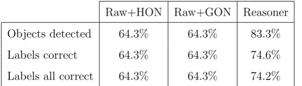
These figures show that use of the spatio-temporal consistency algorithm re-sults in a significant improvement in the object recognition accuracy of the tracker. However, enhancement obtained by this method is fully effective in the case of multiply occupied boxes. Hence it is useful to divide up the statistics into single and multiple box cases. Of the 612 boxes compared, 377 contained a single object (i.e. a person or the ball) and 235 contained multiple objects. The single occupancy box statistics are as follows:

Raw+HON Raw+GON Reasoner

Objects detected 64.3% 64.3% 83.3%

Labels correct 64.3% 64.3% 74.6%

Labels all correct 64.3% 64.3% 74.2%

Fig. 9. Accuracy statistics for boxes containing one object (in ground truth)

This table is somewhat degenerate. This is because both raw data interpre-tations almost invariably assign a single label to single occupancy boxes. The reasoner is considerably more accurate, although it sometimes assigns more than one label to a single occupancy box.

The multiple box statistics give a much more informative comparison. It will be seen in particular that the exact match score for the spatio-temporal consis-tency algorithm is over 60%; whereas, even when magically given the ground occupancy, the raw output of the recogniser rarely gives a completely cor-rect labelling. Without being given the occupancy our heuristic interpretation didn’t give a single completely correct assignment for any multiply occupied box.

12_{The reason this is less than 100% is that the ranked list of likely objects returned}

Raw+HON Raw+GON Reasoner

Objects detected 28.9% 60.4% 81.2%

Labels correct 64.8% 61.8% 89.5%

Labels all correct 0% 13.8% 60.4%

Fig. 10. Accuracy statistics for boxes with more than one object (in ground truth)

7 Discussion and Future Work

The results presented in the previous section show the substantial improve-ment in labelling performance that can be achieved by applying our two sim-ple spatio-temporal consistency rules and using voting over spatio-temporally equivalent regions. The framework presented in this paper is a simple, yet efficient, method of applying these constraints. The performance increase is especially evident in the labelling of multiple occupancy blobs. This is as to be expected as the classifiers were only trained on well separated objects and there is often significant occlusion. The constraints detect the inconsistencies caused by such errors and so can fix qualitatively localised errors.

A possible extension to the system is to the use of multiple cameras. Each (rectangular) blob represents a quadrilateral area when projected to a ground-plane. This area must contain the set of objects relating to the set of labels assigned to the blob. If there are multiple cameras the intersections of these quadrilaterals must contain the intersection of the two label sets. This is a highly efficient way of performing multiple camera integration and occlusion reasoning.

The underpinning theoretical framework could also be usefully generalised in various ways. In particular we would like to remove the assumption that we are dealing with a fixed finite number of labels each of which refers to a unique object. More generally we would like a system which handled classifiers that could apply to multiple objects (for example, to identify team membership in a sports game, or types of animal amongst a mixed herd). In such a setting we need to drop the ‘exclusivity’ constraint employed by our system; and so allow the same label to be simultaneously applied to several envelopes (in fact we would need also to allow multiple instances of a label to be associated with a single envelope). This would obviously weaken the constraints that our system uses and is likely to make our system less accurate. However, the continuity constraint would still be in force, and would still provide a significant mechanism for enhancing the labelling.

a fixed set of objects, we could initially construct only models with a minimal number of objects — i.e. one object in each initial envelope. If an an envelope splits, we will then be forced to recognise that it contains at least two objects. One solution would then be to simply re-generate all possible models from the beginning, but raising the number of objects in the models by one. This would work in off-line mode but is very inefficient. A preferable alternative would be to somehow revise the models already generated in order to add an extra object. For instance, one could consider all possible classifications of the new object and propagate these back along possible paths of the existing envelope sequence in order to generate an set of augmented models including the extra object. This idea introduces some subtleties and is a subject for future work.

A final and more radical enhancement would be to follow up the suggestion made in section 2, which was to implement some kind of feedback between the continuity reasoner and the tracking and classifying modules. In the case of tracking, we have seen that certain tracking errors can be circumvented by the construction of spatio-temporally consistent models. For instance, we can enforce the requirement that objects cannot spontaneously appear or dis-appear. In the current implementation we just take the tracker’s output and attempt to clean up any discontinuities; but it could clearly be useful to signal these back to the tracker so it could modify its processing. For example, the reasoner could flag a tracked box as being almost certainly a phantom, or it could help it keep tabs on objects that remain stationary for long periods of time.

It is less obvious how to achieve feedback between the consistency checking algorithm and the classifier; however, this may also be a very fruitful line of research. The observation that a certain combination of visual properties forms a coherent entity that moves continuously in space is good evidence that those properties serve to identify a particular object. Thus, spatio-temporal continuity can be used as a criterion for validating a classifier: good object classifiers ought to pick out spatio-temporally continuous regions in a video sequence. Hence, one can envisage that spatio-temporal reasoning may play a very important role in the automated learning of object classifiers.

8 Acknowledgements

This work was funded by the European Union under the Cognitive Vision Project (Contract IST-2000-29375).

References

[1] D. Koller, J. Weber, J. Malik, Robust multiple car tracking with occlusion reaasoning, in: Proc. European Conference on Computer Vision, 1994, pp. 189– 196.

[2] M. Isard, A. Blake, Condensation-conditional density propagation for visual tracking, International Jour. of Computer Vision 29 (1998) 5–28.

[3] A. Pece, A. Worrall, Tracking with the EM contour algorithm, in: Proc. European Conference on Computer Vision, 2002, pp. 3–17.

[4] A. Elgammal, L. Davis, Probabilistic framework for segmenting people under occlusion, in: Proceedings of the 8th International Conference on Computer Vision, IEEE, 2001, pp. 9–12.

[5] C. Stauffer, Estimating tracking sources and sinks, in: Proc. IEEE Workshop on Event Mining, 2003.

[6] M. Xu, J. Orwell, L. Lowey, D. Thirde, Architecture and algorithms for tracking football players with multiple cameras, IEE Proceedings: Vision, Image and Signal Processing 152(2) (2005) 232–241.

[7] P. Remagnino, A. Baumberg, T. Grove, D. Hogg, T. Tan, A. Worrall, K. Baker, An integrated traffic and pedestrian model-based vision system, in: Proc. British Machine Vision Conference, 1997, pp. 380–389.

[8] R. Rosales, S. Sclaroff, Improved tracking of multiple humans with trajectory prediction and occlusion modeling, in: Proc. IEEE Workshop on the Interpretation of Visual Motion, 1998.

[9] I. Haritaoglu, D. Harwood, L. Davis, W4: Who? when? where? what? a real time system for detecting and tracking people, in: Proc. International Conference on Automatic Face and Gesture Recognition, 1998, pp. 222–227.

[10] S. Dockstader, A. Tekalp, Multiple camera fusion for multi-object tracking, in: Proc. IEEE Workshop on Multi-Object Tracking, 2001.

[11] C. Needham, R. Boyle, Tracking multiple sports players through occlusion, congestion and scale, in: Proc. British Machine Vision Conference, 2001, pp. 93–102.

[12] S. McKenna, S. Jabri, Z. Duric, A. Rosenfeld, H. Wechsler, Tracking groups of people, Computer Vision and Image Understanding 80(1) (2000) 42–56.

[13] J. Sherrah, S. Gong, Resolving visual uncertainty and occlusion through probabilistic reasoning, in: Proc. British Machine Vision Conference, 2000, pp. 252–261.

[15] A. Lipton, H. Fujiyoshi, R. Patil, Moving target classification and tracking from real-time video, in: Proc. IEEE Workshop on Applications of Computer Vision, 1998, pp. 8–14.

[16] C. Stauffer, W. Grimson, Adaptive background mixture models for real-time tracking, in: Proc. Computer Vision and Pattern Recognition, 1999, pp. 246– 252.

[17] C. Stauffer, E. Grimson, Learning patterns of activity using real-time tracking, IEEE Transactions on Pattern Analysis and Machine Intelligence 22(8) (2000) 747–757.

[18] D. R. Magee, Tracking multiple vehicles using foreground, background and motion models, Image and Vision Computing 20(8) (2004) 581–594.

[19] K. Toyama, J. Krumm, B. Brumitt, B. Meyers, Wallflower: Principles and practice of background maintenance, in: Proc. International Conference on Computer Vision, 1999, pp. 255–261.

[20] H. Sidenbladh, M. Black, L. Sigal, Implicit probabilistic models of human motion for synthesis and tracking, in: Proc. European Conf. on Computer Vision, Vol. 1, 2002, pp. 784–800.

[21] T. Cootes, G. Edwards, C. Taylor, Active appearance models, in: Proc. European Conference on Computer Vision, Vol. 2, 1998, pp. 484–498.

[22] D. Ha, J. Lee, Y. Kim, Neural-edge-based vehicle detection and traffic parameter extraction, Image and Vision Computing 22(11) (2004) 899–907.

[23] J. Heikkila, O. Silven, A real-time system for monitoring of cyclists and pedestrians, Image and Vision Computing 22(7) (2004) 563–570.

[24] C. Needham, P. Santos, D. R. Magee, V. Devin, D. C. Hogg, A. G. Cohn, Protocols from perceptual observations, Artificial Intelligence(To Appear).

[25] D. S. Weld, J. De Kleer (Eds.), Readings in Qualitative Reasoning About Physical Systems, Morgan Kaufman, San Mateo, Ca, 1990.

[26] D. A. Randell, Z. Cui, A. G. Cohn, A spatial logic based on regions and connection, in: Proc. 3rd Int. Conf. on Knowledge Representation and Reasoning, Morgan Kaufmann, San Mateo, 1992, pp. 165–176.

[27] B. Bennett, A categorical axiomatisation of region-based geometry, Fundamenta Informaticae 46 (1–2) (2001) 145–158.

[28] A. G. Cohn, S. M. Hazarika, Qualitative spatial representation and reasoning: An overview, Fundamenta Informaticae 46 (1-2) (2001) 1–29.

[29] J. F. Allen, An interval-based representation of temporal knowledge, in: Proceedings 7th IJCAI, 1981, pp. 221–226.

[31] B. Bennett, A. G. Cohn, P. Torrini, S. M. Hazarika, Describing rigid body motions in a qualitative theory of spatial regions, in: H. A. Kautz, B. Porter (Eds.), Proceedings of AAAI-2000, 2000, pp. 503–509.

[32] B. Bennett, A. G. Cohn, F. Wolter, M. Zakharyaschev, Multi-dimensional modal logic as a framework for spatio-temporal reasoning, Applied Intelligence 17 (3) (2002) 239–251.

[33] J. Fernyhough, A. G. Cohn, D. C. Hogg, Constructing qualitative event models automatically from video input, Image and Vision Computing 18 (2000) 81–103.

[34] A. Galata, A. G. Cohn, D. R. Magee, D. C. Hogg, Modeling interaction using learnt qualitative spatio-temporal relations and variable length markov models, in: F. van Harmelen (Ed.), Proc. European Conference on Artificial Intelligence (ECAI’02), 2002, pp. 741–745.

[35] C. Hudelot, M. Thonnat, A cognitive vision platform for automatic recognition of natural complex objects, in: IEEE (Ed.), International Conference on Tools with Artificial Intelligence, ICTAI, Sacramento, 2003.

[36] P. Santos, M. Shanahan, A logic-based algorithm for image sequence interpretation and anchoring., in: IJCAI, Acapulco, 2003, pp. 1408–1412.

[37] B. Neumann, T. Weiss, Navigating through logic-based scene models for high-level scene interpretations., in: ICVS, 2003, pp. 212–222.

[38] Z. Cui, A. G. Cohn, D. A. Randell, Qualitative simulation based on a logical formalism of space and time, in: Proceedings of AAAI-92, AAAI Press, Menlo Park, California, 1992, pp. 679–684.

[39] R. Howarth, H. Buxton, Conceptual descriptions from monitoring and watching image sequences, Image and Vision Computing 18 (2000) 105–135.

[40] R. E. Bellman, Dynamic Programming, Dover Publications, Incorporated, 2003.